Abstract
When a medium–low-speed (MLS) maglev train is braking, part of its regenerative braking (RB) power consumption may cause a significant rise in the positive rail (PR) voltage. For RB energy re-utilization, an RB energy feedback system (RBEFS) is a promising application, but there is still no specific research in the field of MLS maglev trains. From this perspective, this article focuses on identifying the PR voltage rise behavior and investigating the application of an RBEFS on the over-voltage inhibition. Some development trends of the MLS maglev train, including the DC 3 kV traction grid system and the speed being raised to 160~200 km/h, are also considered in the analyzed scenarios. At first, a modeling scheme of a detailed vehicle–grid electrical power model with the RBEFS is established. On this basis, the PR voltage rise characteristics are analyzed with consideration of three pivotal influencing factors: RB power, PR impedance and supply voltage level. Subsequently, to stabilize the PR voltage fluctuations, the influence rules of the RBEFS on the voltage rise and the mutual transient voltage influences under the operating status switching for multiple vehicles running on the same power supply section are analyzed.
1. Introduction
Construction of a medium–low-speed (MLS) maglev trunk line is one of the most important trends of rail transit in the future. Because the MLS maglev line is short and the station layout is relatively dense, acceleration and deceleration of the maglev train (MT) are frequent. When the MT is in its regenerative braking (RB) state, the part of short-time RB power consumption that cannot be absorbed by other MTs or auxiliary devices will be fed back to the traction grid. If such excessive energy is not properly treated, a significant traction grid voltage rise, i.e., positive rail (PR) voltage rise, is easily caused, which results in vehicle–grid over-voltage, insulation failure and worse power quality [1,2].
Many scholars have studied the features and utilization of RB energy consumption of electric transportation systems. The related research focuses on the high-speed railway (HSR) and the metro so far [3,4,5]. Although the MLS maglev possesses great development prospects, there are still relatively few lines in commercial operation, and there are relatively very few research documents related to the MLS maglev RB. However, the MLS maglev is different from the HSRs and metros with a wheel rail system, as a linear induction motor (LIM) is adopted. The train body is suspended on the F rail, and the train is driven by the electromagnetic force during MT runs. Because the motor air gap of the MLS maglev is relatively much larger and the feedback RB electric power decreases as the motor air gap increases [6], the grid voltage rise behavior of the MLS maglev is different from those with a rotating motor and needs to be clarified.
Further, the increases in the running speed and the supply voltage level are two important development trends of the MLS maglev. The highest running speed has reached 140 km/h in the Chinese Changsha maglev line. However, the development of the MLS maglev to a connection line between a city center and suburb area requires a 160~200 km/h speed to accommodate the corresponding functions. In addition, although the supply voltage level of DC 0.75 kV or DC 1.5 kV has been generally adopted, the construction of a DC 3 kV system has excellent prospects due to the advantages of fewer substations, lower traction waste, etc. Some scholars have studied the RB issues of a DC 3 kV traction grid [7,8,9,10]. The main focus has been on energy conservation. The design or improvement of substations, regenerative inverter or energy storage system has been studied in detail to achieve this goal. Nevertheless, the voltage rise in the RB scenario of a DC 3 kV system has not specifically been studied in the relevant literature. Compared to the present highest train speed and supply voltage level of the MLS maglev, both the speed being raised to 160~200 km/h and the voltage being raised to DC 3 kV bring about greater challenges in RB over-voltage control.
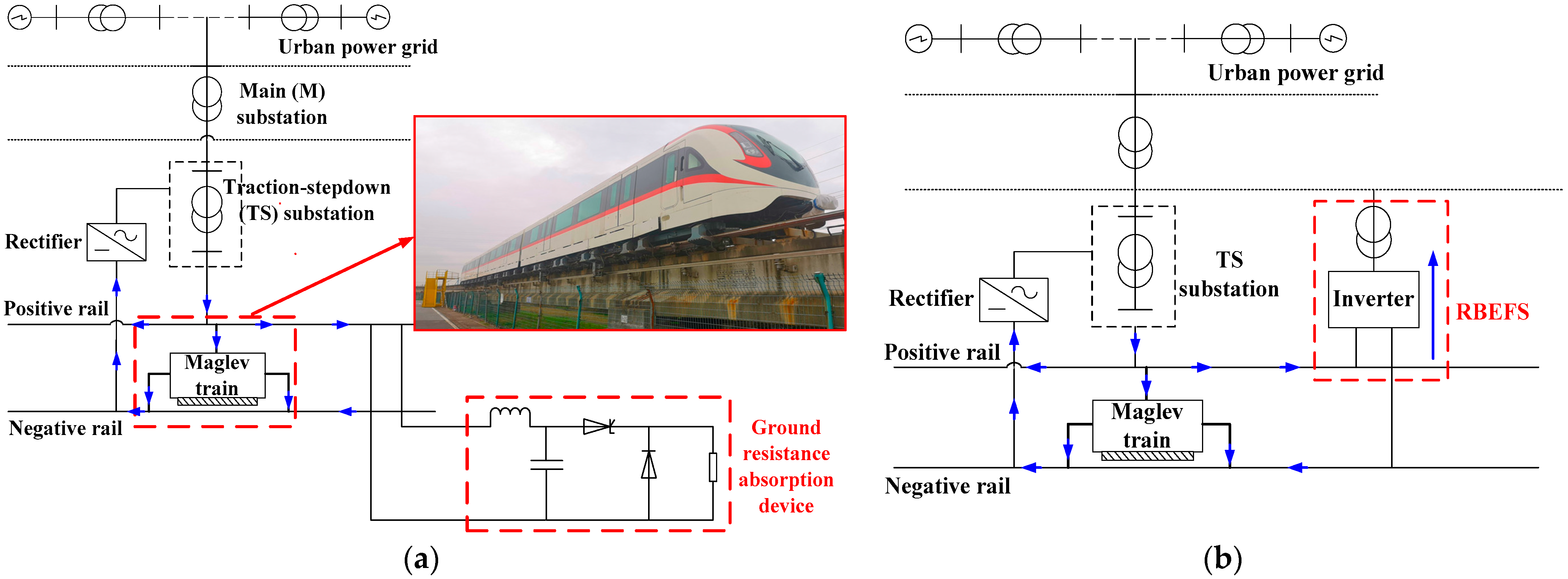
The current treatment method targeted for the MLS maglev is to release the excess RB energy in the form of heat energy via a ground resistance absorption device [11], but it results in energy waste and increases the temperature in the tunnel. To better accommodate the RB energy, measures of energy storage [12,13,14,15] and energy feedback [16,17,18] have been proposed for the various types of railway transit systems. Compared to the energy storage applications, the energy feedback system exerts three advantages: First is the high efficiency. Excessive RB energy can be directly fed back to the AC system through the RBEFS, and the traction grid energy utilization rate can be greatly improved [17,18]. Second is the cheaper price. The energy storage system is relatively large and expensive, and is more suitable for 600 V and 750 V traction grids at present [19,20]; the price of the RBEFS is also becoming cheaper with the development of high-power semiconductor IGBTs. The third is the smaller space. Because the power transistor switching frequency is relatively high, the filter volume capacity can be designed to be relatively small [21]. Therefore, the RB energy feedback system (RBEFS) can be considered a promising application for the MLS maglev. Figure 1a and Figure 1b, respectively, depict the application of different regenerative energy processing methods on the MLS system. Figure 2 displays the site photo of the RBEFS.

Figure 1.
Diagram of MLS maglev electrical power system with different regenerative energy processing methods: (a) resistance absorption device; (b) RBEFS device.
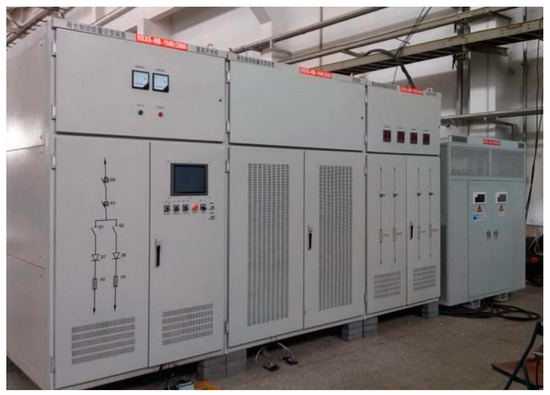
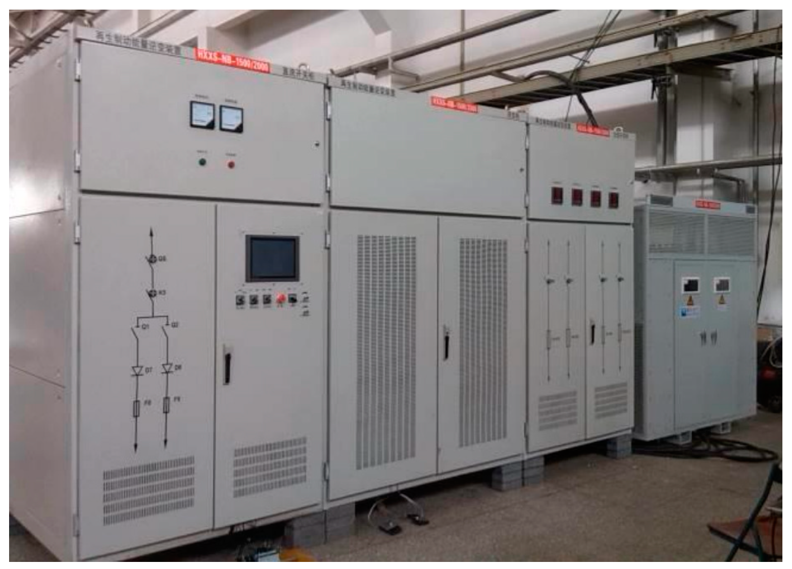
Figure 2.
Site photo of RBEFS of urban rail line.
For the grid voltage rise caused by the RB, relevant research is relatively scarce compared to energy management research. And the on-site test and the software simulation are the main methods. For HSRs, the modeling and simulation of the influences of RB on the catenary voltage were studied on a train passing through a long downhill section [20]. For the metro, the analysis of over-voltage in the DC catenary has predominantly been conducted through simulations [22], and various approaches including train timetable optimization, energy storage systems and feedback systems have been compared to avoid the over-voltages [16]. An important part of these methods such as the control strategy of energy storage systems was also exclusively analyzed or improved by some scholars to control the line voltage [23].
For the application of the RBEFS on the RB influences of electric transport trains, related research focuses on energy conservation rather than controlling grid voltage rise [24]. Mathematical modeling and digital simulation are the main research approaches in terms of suppressing voltage rises. Some scholars have investigated the optimal electrical parameters, action threshold or control strategies of the RBEFS [18,25,26] to achieve the excess energy feedback, mitigate the grid voltage rise and accelerate the steady-state recovery after response. The RBEFS control strategies have been given much attention [27]. In [27], different control schemes were investigated to increase the energy utilization efficiency by adjusting the catenary DC voltage in the inverter. Some scholars have also attempted to design new control schemes considering the grid voltage rise inhibition [26].
In the field of the MLS maglev, there are relatively few relevant studies, and the scholars involved have only implemented the theoretical study on the application of braking resistance and super-capacitor energy storage devices, and the optimization of operational diagram, with the purpose of lowering energy consumption [11,28]. In the above studies, the grid voltage rise has not been addressed; their focus is on the traction grid rather than train, and the vehicle part is very simplified in the modeling; there is no research on the application of an inverter RBEFS.
Figure 3 shows the limitations of previous relevant research and works and those of this article. As an extension of previous works, this article focuses on the modeling of the MLS maglev vehicle–grid electric power system with an inverter RBEFS. The PR voltage rise and its inhibition with the RBEFS are evaluated considering the different RB scenarios. The contributions of this study can be summarized as follows.
- (1)
- A detailed modeling scheme of the vehicle–grid electrical power system with the RBEFS is established for the MLS maglev. The maglev motor characteristics are incorporated to accurately present the difference between wheeled and maglev transport, and the AC properties and energy dispersal path are considered in detail.
- (2)
- Important development prospects of the MLS maglev, namely, the DC 3 kV traction grid and 160~200 km/h vehicle speed, are firstly considered influence factors to reveal the grid voltage rise behavior and the influence of over-voltage inhibition with the RBEFS.
The remainder of this article is organized as follows. In Section 2, a modeling scheme of a vehicle–grid electrical power system with the RBEFS is proposed. Then, the PR voltage rise behavior is analyzed with consideration of three pivotal influencing factors, RB power, PR impedance and supply voltage level, in Section 3. In Section 4, multiple operating scenarios are further considered, and the effect of the inverter RBEFS on the PR voltage rise inhibition is investigated. Conclusions are drawn in Section 5.
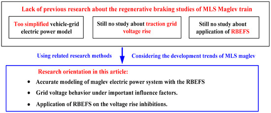

Figure 3.
Limitations of previous research [11,28] and research orientation of this article.
Figure 3.
Limitations of previous research [11,28] and research orientation of this article.
2. Vehicle–Grid Electrical Power Modeling Considering the RBEFS
A typical Chinese MLS maglev line is taken as an example, and a model for the vehicle–grid electrical power system with the RBEFS is established in this section. The model contains the vehicle–grid part and the RBEFS part. A DC 3 kV voltage level and a 160 km/h~200 km/h MT speed are also included.
2.1. Modeling of the Vehicle–Grid Electrical Power System
2.1.1. Traction Grid Part
The running of the MLS maglev train requires frequent acceleration and deceleration, leading to rapid fluctuations in traction current amplitudes across a wide range. Moreover, changes in current direction occur within the reflex system as the train’s position shifts or when the RB initiates. These factors indicate that the DC rail transit electrical power system exhibits AC characteristics. To ensure precise calculation results, the model must consider not only resistance parameters but also AC properties, involving PR inductance (L0), PR capacitance-to-ground (C0) and coupling conductance between PR and negative rail (NR) voltage (C12). L0 is determined to be equal to μ/8π, where μ represents rail permeability, while C0 and C12 are derived according to [29].
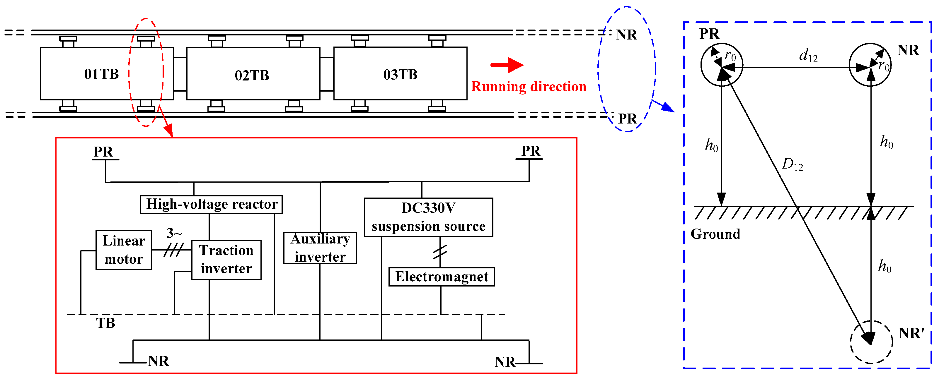
where Ɛ0 is the rail dielectric coefficient, h0 is the rail height, r0 is the rail radius, d12 is the distance between PR and NR, and D12 is distance between PR and image of NR.
The original parameters of the Chinese Changsha MLS operation maglev line are considered the standard original parameters for the modeling and estimating in this article. The rail-earth leakage resistance G0 is extremely large and its unit length value is set to 107 Ω/m based on the line. Because the contact rail material is steel–aluminum alloy and the rail area is almost 82 cm2, the unit length conductor rail resistance R0 is set to 0.16279 Ω/km. As depicted in Figure 4, each train body (TB) carries two pairs of collector shoes and one MT is composed of three TBs. NR’ is the image of NR. The distance between two collector shoes in the same TB is about 5.9 m, while the distance between two adjacent collector shoes in the adjacent TBs is around 6.6 m.
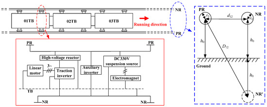
Figure 4.
Electrical structure and equipment layout of MLS MT.
2.1.2. Vehicle Part
The MT traction drive system is elaborately constructed. As depicted in Figure 4, the MT is suspended using a combination of several electromagnet coils, with electromagnetic force being produced by a compact LIM [30]. Each frame is fitted with one LIM stator and two inverters. The LIM rotor, distributed along the running track, corresponds to the expanded secondary side of the rotating motor.
The motor is approximated by the rotating motor module, ensuring that its input and output characteristics align with those of the LIM. The output rated power and frequency range are 68.3 kVA and 4 kHz, respectively. In comparison to the rotating motor, the LIM has a larger air gap, leading to increased excitation consumption and additional end effects. Consequently, this results in a lower power factor and reduced efficiency [31]. Considering these factors, the power factor and efficiency are established at 0.65 and 0.6, respectively.
In addition, the position of each drive unit on the TB is involved. In the analyzed maglev line, the constant slip-frequency control mode is adopted in the inverter and each TB carries five suspension frames. The copper wire with the 120 mm2 area is used to connect adjacent TBs and its resistance is considered between adjacent TB modules.
2.2. Modeling of the RBEFS
A three-phase voltage-type PWM inverter that is widely used in urban rail transit is considered the RBEFS in the model. It is composed of a PWM inverter, filter, isolation transformer, rectifier transformer, SVPWM pulse trigger module and inverter drive module. The inverter aims to invert the traction grid DC voltages into the three-phase AC voltages. The filter aims to lower the harmonic contents in the current feedback. The isolation transformer aims to avoid the direct flow of the DC-side current into the AC system under the short-circuit fault. The three-phase bridge IGBT/Diodes inverter is adopted and the transformer transformation ratio at the grid side is set to 1180 V/35 kV.
In the model of the PWM inverter, Equation (2) is required for the capacitance value at the IGBT DC side to meet the voltage tracking speed requirement and limit the load disturbance exerted on the power system as much as possible.
where is the time required for the DC-side voltage to rise from the initial value to the rated value; RL is the load rated resistance; Udc is the DC-side voltage; ΔUmax is the maximum allowable voltage fluctuation range on the DC side. Due to the above limitations and the factors of overall dimension, cost and service life, I set C = 20,000 μF.
The inductance value at the IGBT AC-side meets the requirements of (3).
where TS is the switching cycle; Usm is the maximum voltage value at the AC side; Δimax is the allowable maximum current fluctuation value, usually 10% of the rated value of the medium-voltage grid; φ is the AC-side phase angle; PL is the converter rated power.
The regulation method of the SVPWM and digital proportional integral PI control of the voltage outer loop and current inner loop are adopted in the control circuit. In the filter model, the LCL-type filter is involved due to the favorable filtering effect.
In Figure 5, L1 and Lg in order are the inductances of the inverter side and isolation transformer side. The transfer function is calculated as
The designed resonant frequency of the RBEFS should be large enough to avoid the resonance and the following principles need to be satisfied.
- (1)
- The voltage drop caused by the filter inductance is larger than or equal to 10% of the medium-voltage grid rated voltage.
- (2)
- The resonance peak value should appear in the medium-frequency band. Therefore, the resonant frequency, fres, shall meet the following requirement:
The on–off frequency of the switching device is the main reason for the harmonics generated during the action of the inverter. To weaken the harmonics and import the high-frequency current parts into the capacitance, the capacitive reactance of Cg shall satisfy Equation (6). Meanwhile, since the reactive power should be less than 5% of the rated power, the value of Cg should meet Equation (7).
where λ is the ratio of the fundamental reactive power to the active power; P is the active power rated value; f1 is the switching frequency; Em is the traction grid phase voltage.
Considering the above, L1, Lg and Cg are, respectively, set to 0.65 mH, 0.15 mH and 300 μH.

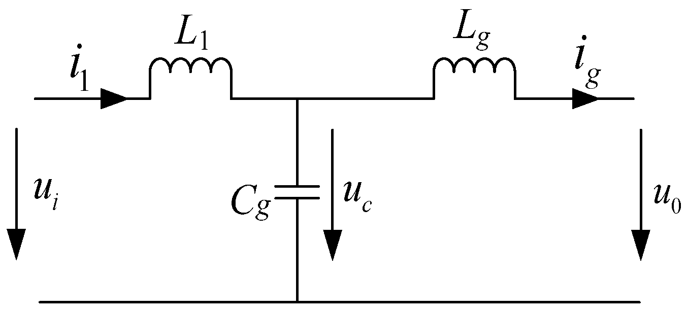
Figure 5.
Diagram of undamped single-phase topology of LCL filter.
Figure 5.
Diagram of undamped single-phase topology of LCL filter.
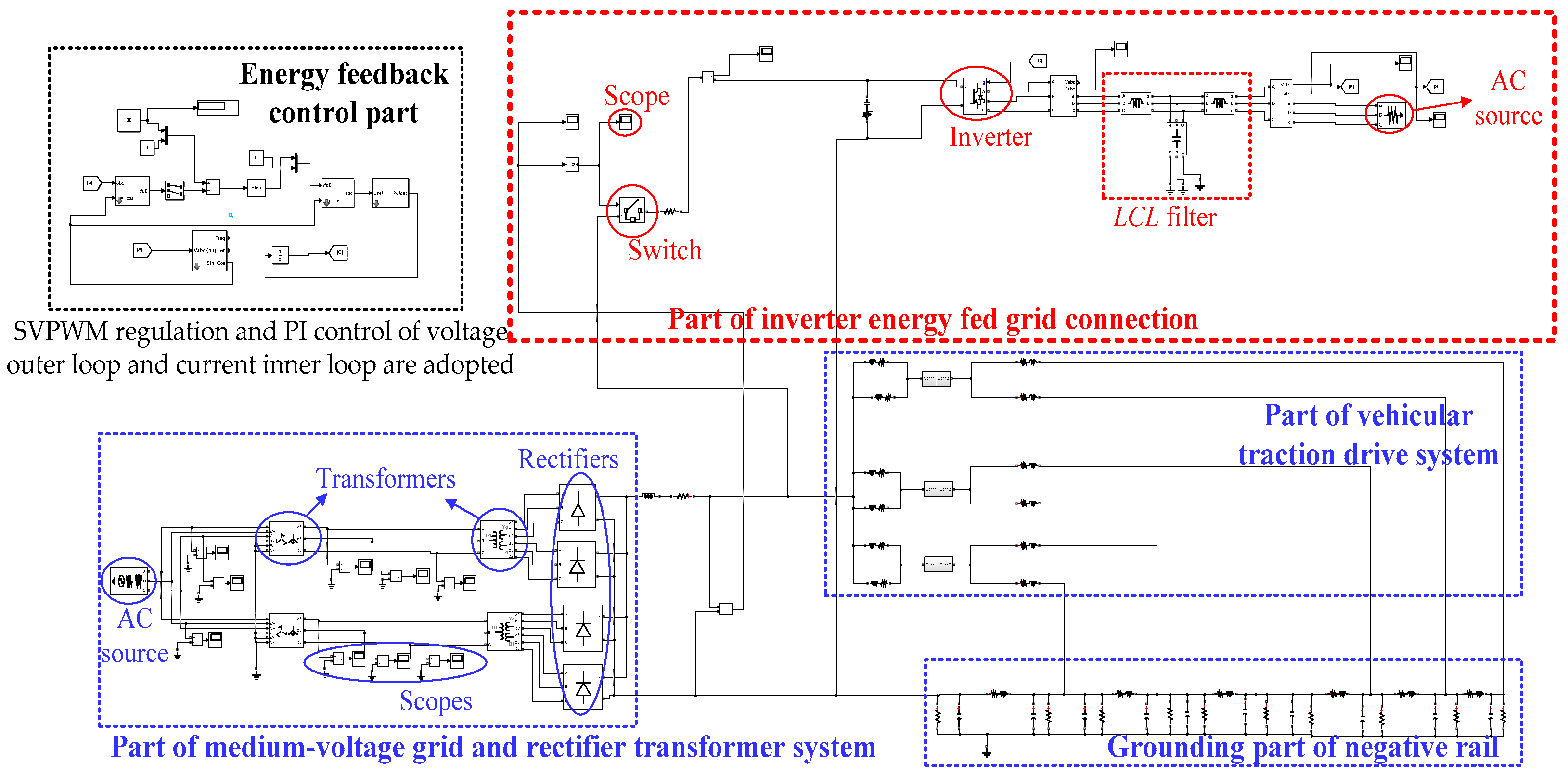
2.3. Integration Model and Its Verification
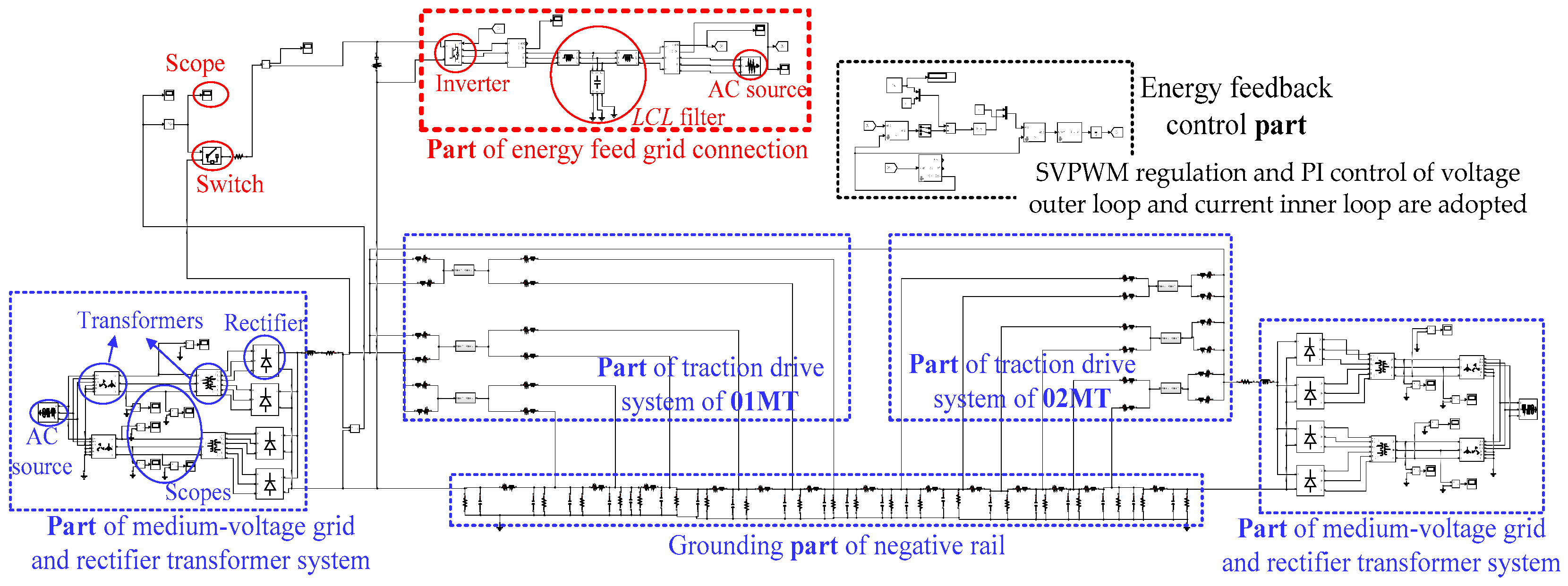
Combining the above two parts, the final model of the electrical power system with the RBEFS is built using the MATLAB/Simulink software 2016a package, as seen in Figure 6. In the part of the vehicular traction drive system, the target commands of output torque and rotor speed are set to simulate the running scenarios of traction, coasting and braking and their time.

Figure 6.
Vehicle–grid electrical power simulation model of MLS maglev considering RBEFS.
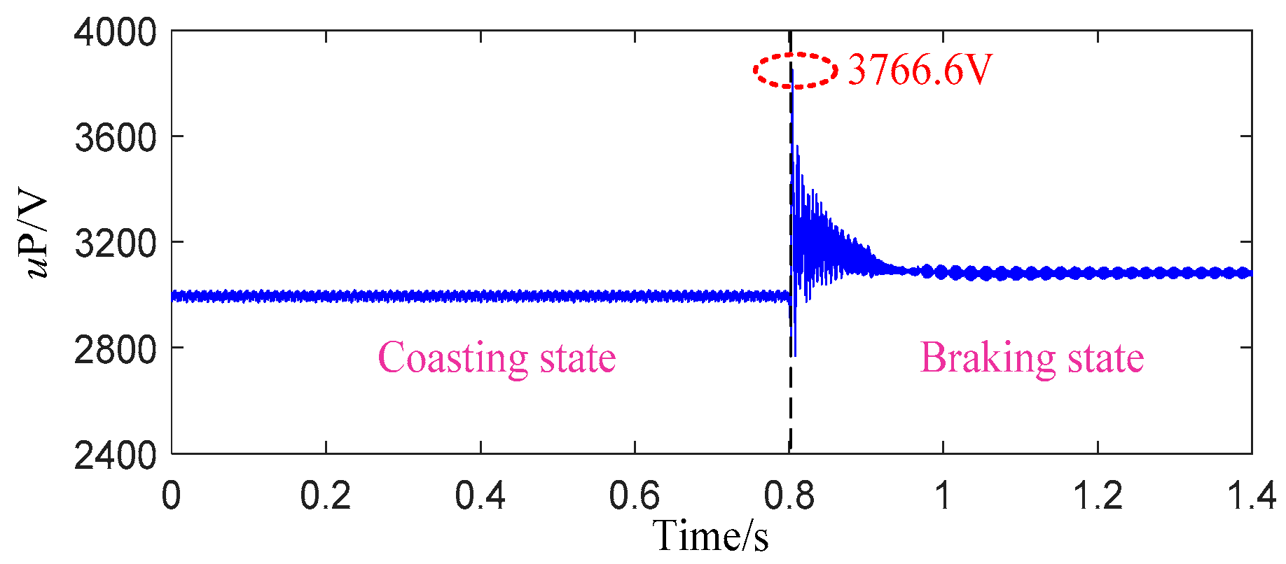
In this paper, the PR voltage is marked as uP and its maximum value is uPmax. Let us assume that the supply voltage is 3000 V and the RB is generated at 0.8 s, where the MT speed is reduced from 200 km/h to 50 km/s. The simulation results of the equivalent rotor speed v0, the equivalent motor output torque Te and uP are shown in Figure 7 and Figure 8. As RB occurs, v0 is adjusted from 135 rad/s to 30 rad/s, Te is changed into a negative value and its maximum absolute value reaches 2189.8 N·m. For v0, Te and uP, their amplitude variation tendencies during the RB should be consistent for the MLS maglev and the metro due to the similar DC traction electrical power supply system. Therefore, by comparing the waveforms of Figure 7 and Figure 8 with those of a metro train measured in [18], the close similarity proves the validity and feasibility of the presented model.
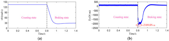
Figure 7.
Simulation results of equivalent rotor speed v0 and equivalent motor output torque Te when RB generates at 0.8 s: (a) v0 curve; (b) Te curve.

Figure 8.
Simulation results of PR voltage fluctuation when RB state generates at 0.8 s.
3. Analyses of Positive Rail Voltages under Multiple Interfering Factors
The electric energy flow direction is from a high potential to a low potential. As RB energy is returned, since the traction grid voltage at the traction substation is almost unchanged, the PR conductor voltage drop during the transmission of RB energy will inevitably lead to the PR voltage rise at the MT location. Therefore, RB power, PR impedance and substation voltage level are three pivotal factors affecting the voltage rise. The model built in Section 2 is used to analyze the influence of these three factors in this section. The maximal voltage rise percentage compared to the average voltage (AVG) amplitude before RB is marked as ΔUP. The total simulation time is 1.4 s and the beginning moment of RB is 0.8 s. The action voltage of the RBEFS U0 is set to 1680 V.
3.1. Influence of RB Power
RB may begin at different MT speeds v and the slope path is inevitable in some maglev lines. In the Chinese Fenghuang MLS maglev line, the lines with the gradients i < 10, 10 ≤ i < 20 and i ≥ 25, respectively, account for 28.83%, 9.03% and 62.14% of the total line, and the highest i is 51 (i represents the thousand fraction ‰ of the ramp gradient). Since both v and i are important variables affecting RB power, the PR voltage rises under the different v and i are analyzed here when the distance from the MT to the substation is set to 2 km and the common traction supply voltage U = 1.5 kV is considered.
3.1.1. Comparison of Different MT Speeds
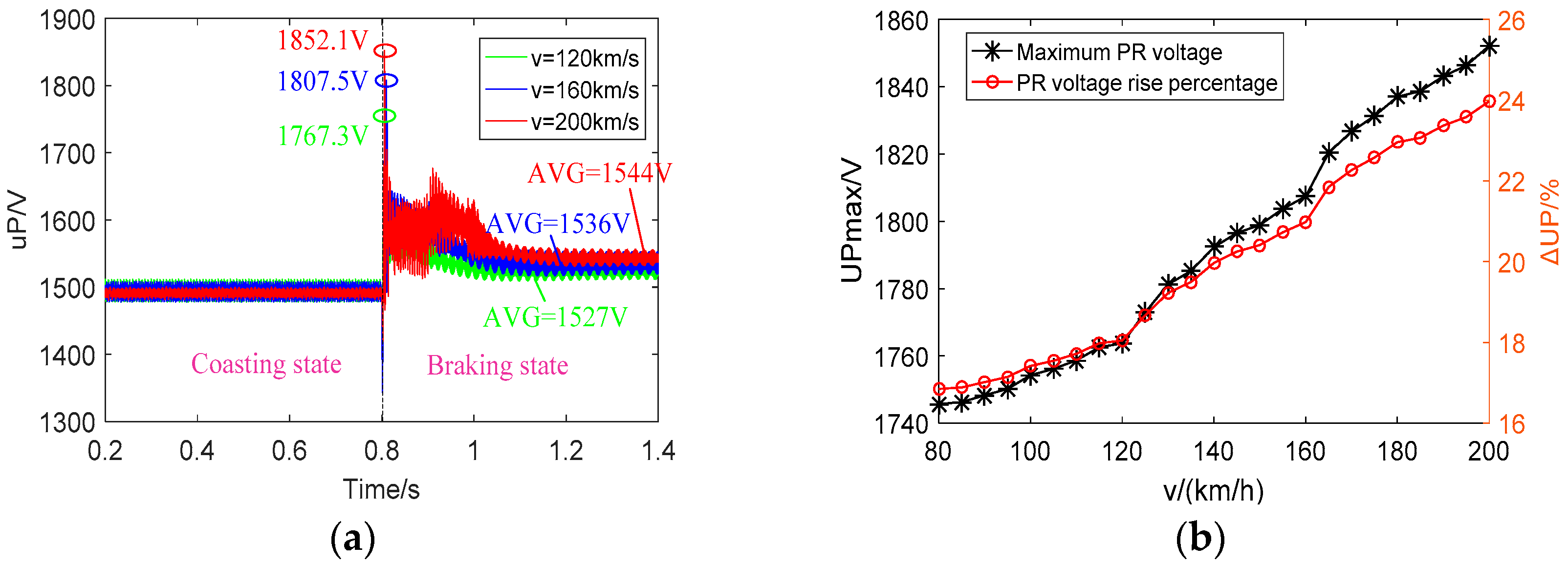
The waveforms of the PR voltage uP under v = 120, 160 and 200 km/h and the relations between the UPmax, the ΔUP and the v of 80~200 km/h are shown in Figure 9. When the MT begins to decelerate at a higher speed, more kinetic energy is available to be converted into electrical energy. Moreover, at higher speeds, the higher efficiency of energy conversion leads to a more effective transfer of energy back to the grid. The above leads to a higher ΔUP, which conforms with the analyzed influence trend in Figure 9b. UPmax is increased from 1746 V to 1852.1 V as v varies from 80 km/h to 200 km/h. And the corresponding ΔUP increases from 16.87% to 23.97%, as shown in Figure 9b. The AVG amplitude after stabilization during RB is higher with the increased v, increasing from 1527 V (v = 120 km/h) to 1544 V (v = 200 km/h), as shown in Figure 9a.

Figure 9.
PR voltages under different train speeds v: (a) PR voltage fluctuations; (b) relation between PR voltages and v.
3.1.2. Comparison of Different Downhill Slope Gradients
As the MT goes downhill at constant speed v, the following relationship is satisfied:
where M is the MT mass, Fb(v) is the braking force required for the MT to run at constant v when the gradient is i‰, Fi is the additional resistance, Fi = i, and F0 is the basic resistance comprising air resistance, the current collector resistance and electromagnetic resistance. F0 is expressed by
where m is each TB mass, f is the current collector resistance, f = μF0, μ is the friction coefficient between the current collector and conductor rail, and F0 is the current collector pressure.
Based on (8), RB power PRB is obtained by PRB = η1η2F0v, where η1 is the generator conversion efficiency and η2 is the energy feedback efficiency from the inverter to the traction grid. Then, motor rotor speed v0 and motor output torque Te under different i are calculated and substituted into the model of Figure 6. The i in the range of −36~−20 is considered to analyze the slope influence on the PR voltage rise when v = 200 km/h is maintained. Their corresponding ω* in the LIM model are shown in Table 1.

Table 1.
Model target command parameter values under different gradients (RB conditions).
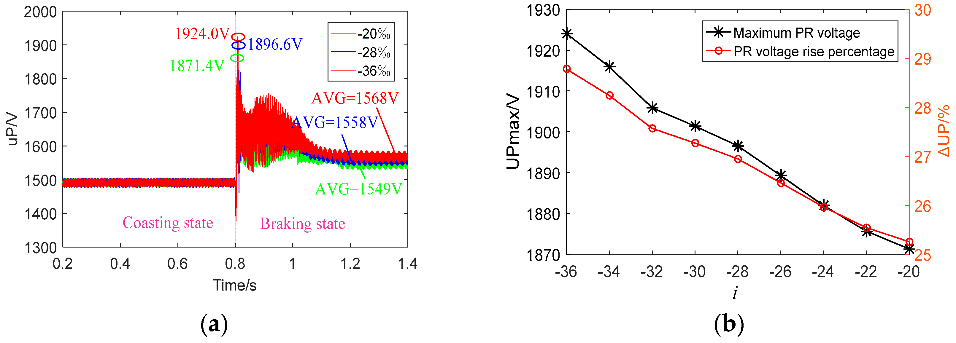
The waveform of UP under i = −20, −28 and −36 and the relationship between Upmax and i are simulated in Figure 10. It is obvious that the steeper slope requires the larger RB power when the MT goes downhill, resulting in a more severe voltage rise. The UPmax (ΔUP) increases from 1871.4 V (25.26%) to 1924.0 V (28.78%) as i = −20~−36, as shown in Figure 10b. The AVG value after stabilization during RB is becomes higher as the downhill becomes steeper, increasing from 1549 V (i = −20) to 1568 V (i = −36), as shown in Figure 10a. By comparing Figure 9 and Figure 10, as v = 200 km/h, the UPmax is 1852.1 V for a smooth road and 1871.4 V for the least steep slope with i = −20. It shows that the voltage rise on the downhill path is higher than that on a smooth road. In addition, I can ascertain from Figure 9b and Figure 10b that the effect of v on the voltage rise is more prominent than the effect of slope.
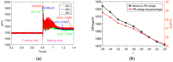
Figure 10.
PR voltages under different slope gradients i: (a) PR voltage fluctuations; (b) relation between PR voltages and i.
3.2. Influence of PR Impedance
For the DC traction grid system, the unit length PR impedance in the whole line can be regarded as a constant value and the distance from the MT to the substation (marked as l) determines the PR impedance. The impedance always changes as the MT runs and thus the PRB is different for the different RB occurrence moments. Therefore, it is necessary to assess the voltage rise range considering the RB occurrence locations. In addition, the traction power supply mode is the second pivotal influencing factors for the impedance. The unilateral power supply mode in the Chinese Xinzhu maglev line and the bilateral power supply mode in the Chinese Changsha maglev line are compared in this part.
3.2.1. Comparison of Different RB Occurrence Locations
A unilateral power supply system is considered. According to the present operation line, l = 0.5~5 km is selected to be analyzed. PR voltage rises under l = 0.5~5 km with 0.5 km intervals are, respectively, simulated and the results are presented in Figure 11.
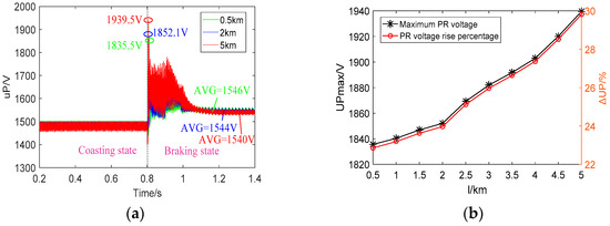
Figure 11.
PR voltages under different RB occurrence locations: (a) PR voltage fluctuations; (b) relation between PR voltages and distance from MT to substation.
As mentioned before, the higher l leads to the higher PR impedance and the higher voltage drop between the substation and MT. As the PR voltage at the substation is almost unchanged at 1500 V, it is obvious that the higher PR voltage drop forms the higher UPmax at the train’s location. Contrary to this rule, the higher line voltage drop enables the lower voltage received by the MT when the train is in the stable interval. It is proven in Figure 11 that the relationship between UPmax and l (1835.5 V, 1852.1 V and 1939.5 V for 0.5 km, 2 km and 5 km) and the relationship between PR stable voltage and l (1546 V, 1544 V and 1540 V for 0.5 km, 2 km and 5 km) are contrasting.
3.2.2. Comparison of Different Power Supply Modes
Assuming that all of the distances from the train to the nearby substations are the same, the PR voltage fluctuations under the unilateral and bilateral power supply modes are compared in Figure 12. Compared to the unilateral mode, the PR impedance between the substation and MT is relatively lower and the PR voltage drop is relatively smaller for the bilateral mode. This results in a higher UPmax and a lower stable PR voltage amplitude during RB. In addition, by comparing Figure 11b and Figure 12b, the influence caused by the power supply mode is significantly lower than that of the RB occurrence location. This proves that more attention should be paid to the RB occurrence position when only the traction grid impedance is considered to lower the voltage rise.
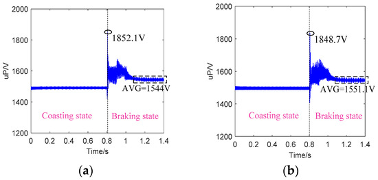
Figure 12.
PR voltage fluctuations under different traction electric power supply modes: (a) unilateral power supply; (b) bilateral power supply.
3.3. Influence of Supply Voltage Level
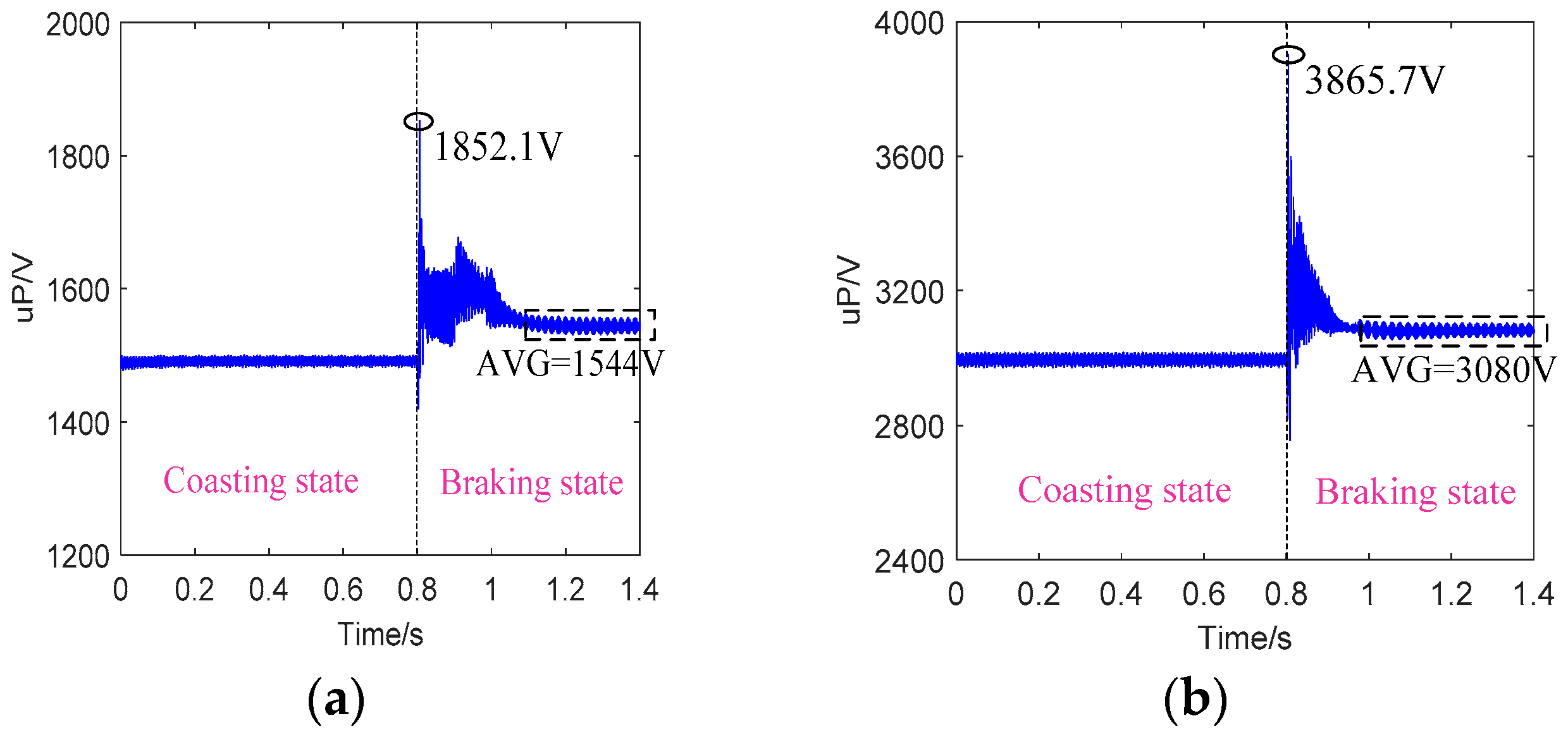
Focusing on the influence of the traction electric power supply mode, the DC 3 kV mode, one development trend of the MLS maglev, is compared with the traditional DC 1.5 kV mode here. According to the results in Figure 13, the UPmax reaches 1852.1 V and 3865.7 V, respectively, which is 23.97% and 28.99% higher than the AVG amplitudes before RB, i.e., 1494 V and 2997 V. This illustrates that the transient voltage rise in the beginning of RB is proportional to the supply voltage.

Figure 13.
PR voltage fluctuations under different traction voltage levels: (a) 1.5 kV; (b) 3 kV.
4. Analyses of Positive Rail Voltage Rises under the RBEFS Influence
The PR voltage rises caused by the multiple RB running scenarios are compared before and after the RBEFS is put into use. The comparisons aim to elucidate the voltage rise inhibition role of the RBEFS. Meanwhile, the development trends of the urban rail system, i.e., DC 3 kV and 160~200 km/h, are involved, and the influences of different supply voltage levels U and MT speeds v on the inhibitions are compared.
4.1. Multiple Cases of Single-Train Operation
The total simulation time, the RB occurrence moment and the distance from the MT to the substation are, respectively, set to 1.4 s, 0.8 s and 2 km. Based on the previous application of the RBEFS, the RBEFS action voltages U0 are, respectively, set to 1680 V and 3360 V for U = 1.5 kV and U = 3 kV.
4.1.1. Different MT Speeds
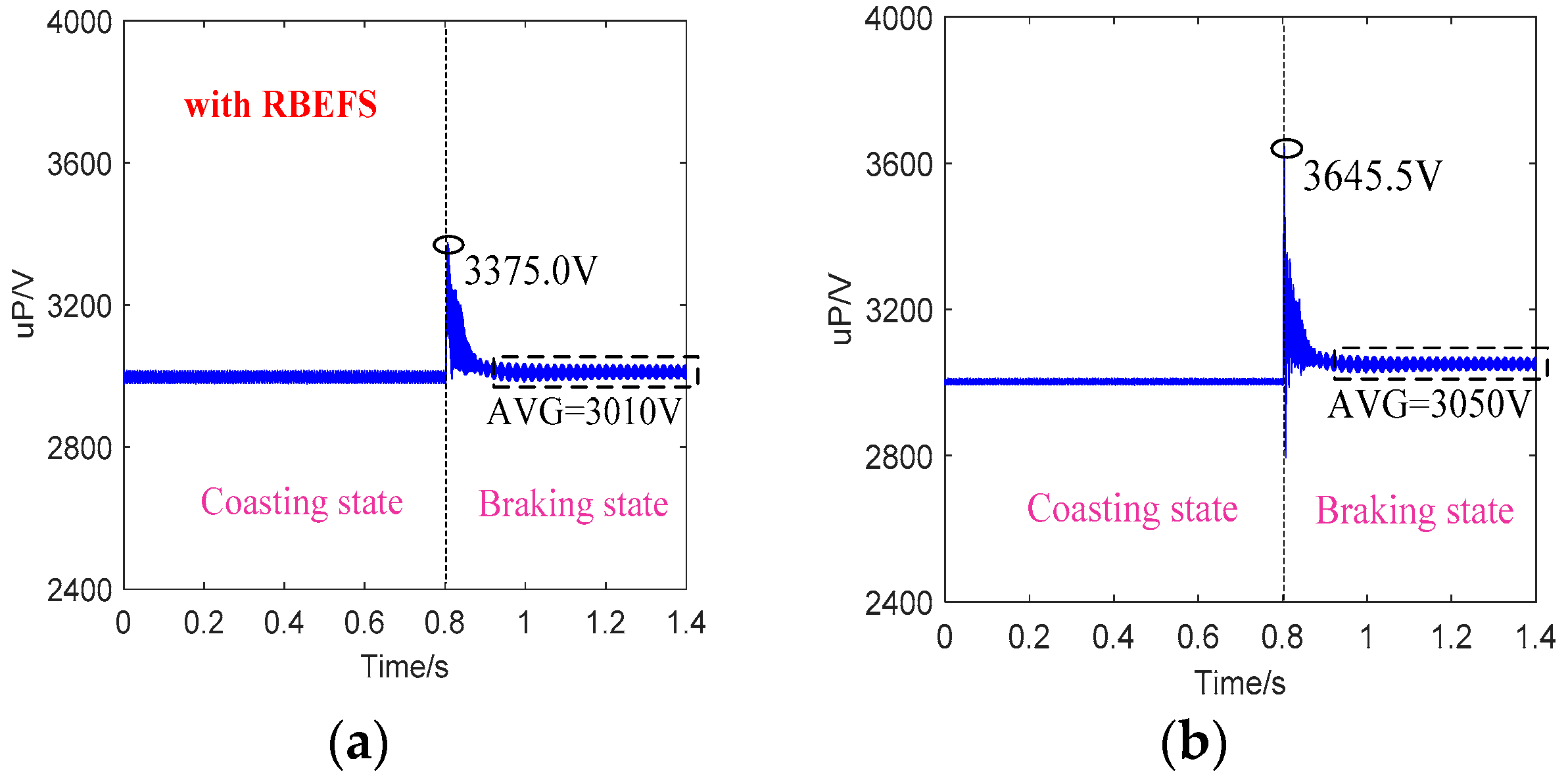
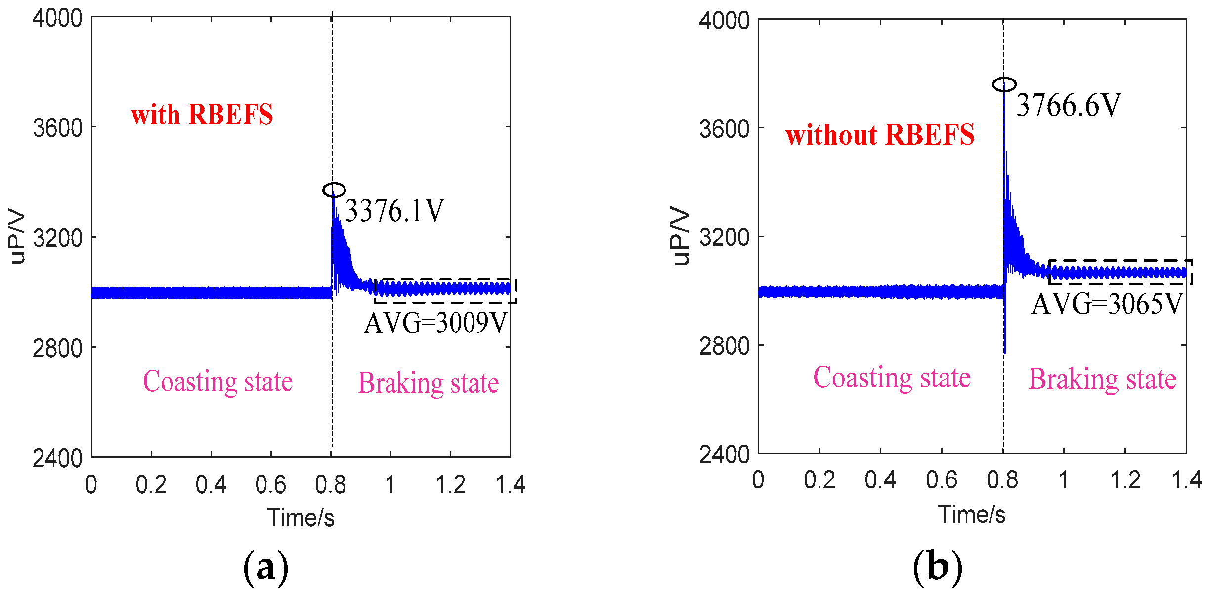
The supply voltage level U is set to 3 kV. Figure 14, Figure 15 and Figure 16 compare the influences of the RBEFS on the PR voltage fluctuations under the different v (120, 160 and 200 km/h). It is observed that the feedback device plays a remarkable role in lowering the voltage rise. As v = 200 km/h, the feedback device reduces the UPmax from 3850.1 V to 3384.8 V. The inhibition comparisons for the ΔUP at v = 80, 120, 160 and 200 km/h are concluded in Table 2, showing that the inhibition percentage keeps increasing as the v increases, both for UPmax or the stable PR voltage amplitude during RB.
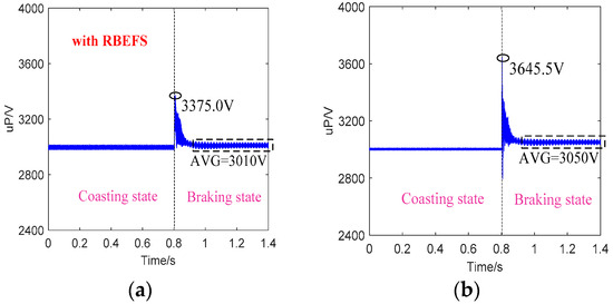
Figure 14.
PR voltage fluctuations when v = 120 km/h: (a) with RBEFS; (b) without RBEFS.
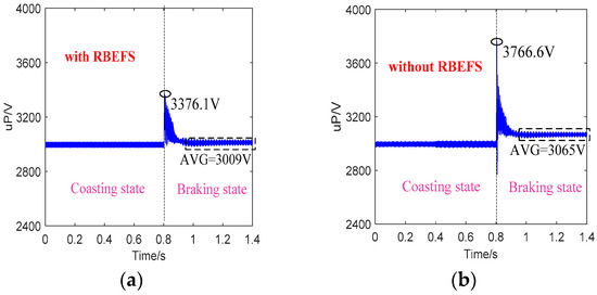
Figure 15.
PR voltage fluctuations when v = 160 km/h: (a) with RBEFS; (b) without RBEFS.
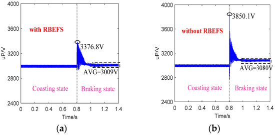
Figure 16.
PR voltage fluctuations when v = 200 km/h: (a) with RBEFS; (b) without RBEFS.
Table 2.
Comparison of PR voltage rise percentages during RB under different v.
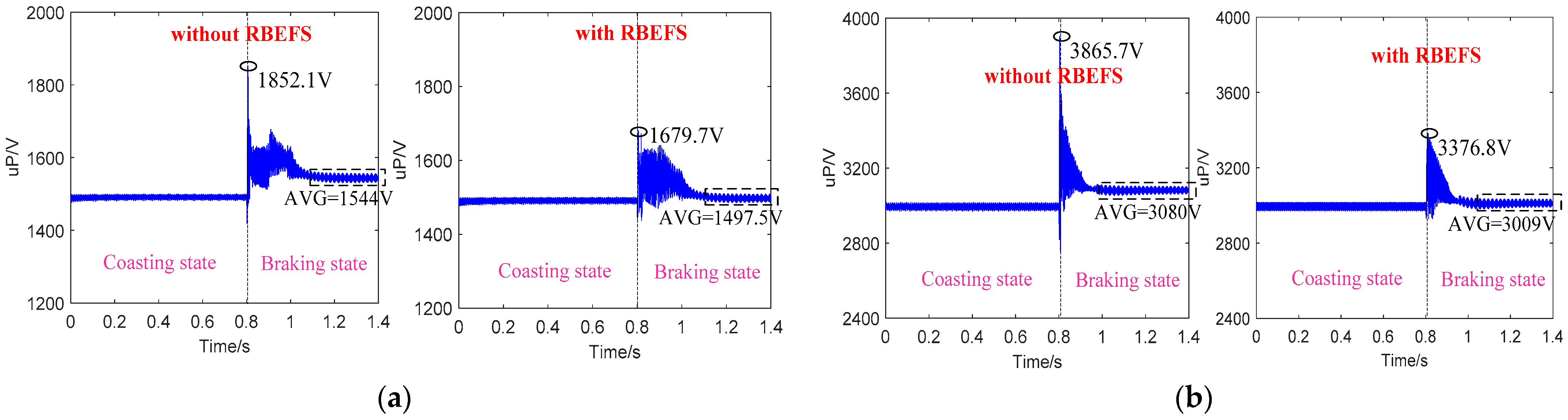
4.1.2. Supply Voltage Levels
Figure 17 shows the analytical results of v = 200 km/h and the traction supply voltages U = 1.5 and 3 kV. Before the feedback device is put into use, the maximal voltage amplitudes in order reach 1852.1 V and 3865.7 V, which are 23.97% and 28.99% higher than the AVG amplitudes before RB. After the feedback device is introduced, the maximal amplitudes in order reach 1679.7 V and 3384.8 V, only 12.43% and 12.67% higher than the AVG amplitudes before RB (see Figure 17). This comparison shows that the inhibition is affected by the U. From Table 3, it can be seen that the inhibition percentage is significant greater as the U is higher for the maximum value at the beginning of RB.
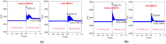
Figure 17.
PR voltage fluctuations under different supply voltage levels with and without the RBEFS: (a) 1.5 kV; (b) 3 kV.
Table 3.
Comparison of PR voltage rise percentages during RB under different U.
4.2. Analyses of Multiple-Train Simultaneous Operation in Same Power Supply Section
The RB cases for the multiple MTs running in the same power supply section are further examined. The over-voltage superimposed influences are analyzed for the case in which two running MTs enter the opposite state (traction state vs RB state) at the same or very close moment. The total simulation time is set to 1.4 s. Because the higher U and higher v result in the higher PRB, I consider the most serious situation and v = 200 km/h, U = 3 kV and U0 = 3360 V are set. Let us assume that two trains are named as 01 MT and 02 MT and their distances to the substation in the same direction are, respectively, 2 km and 3.5 km. Figure 18 shows the established simulation model based on the model of Figure 6.
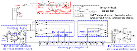
Figure 18.
Vehicle–grid electrical power simulation model considering RBEFS and multiple-vehicle running cases.
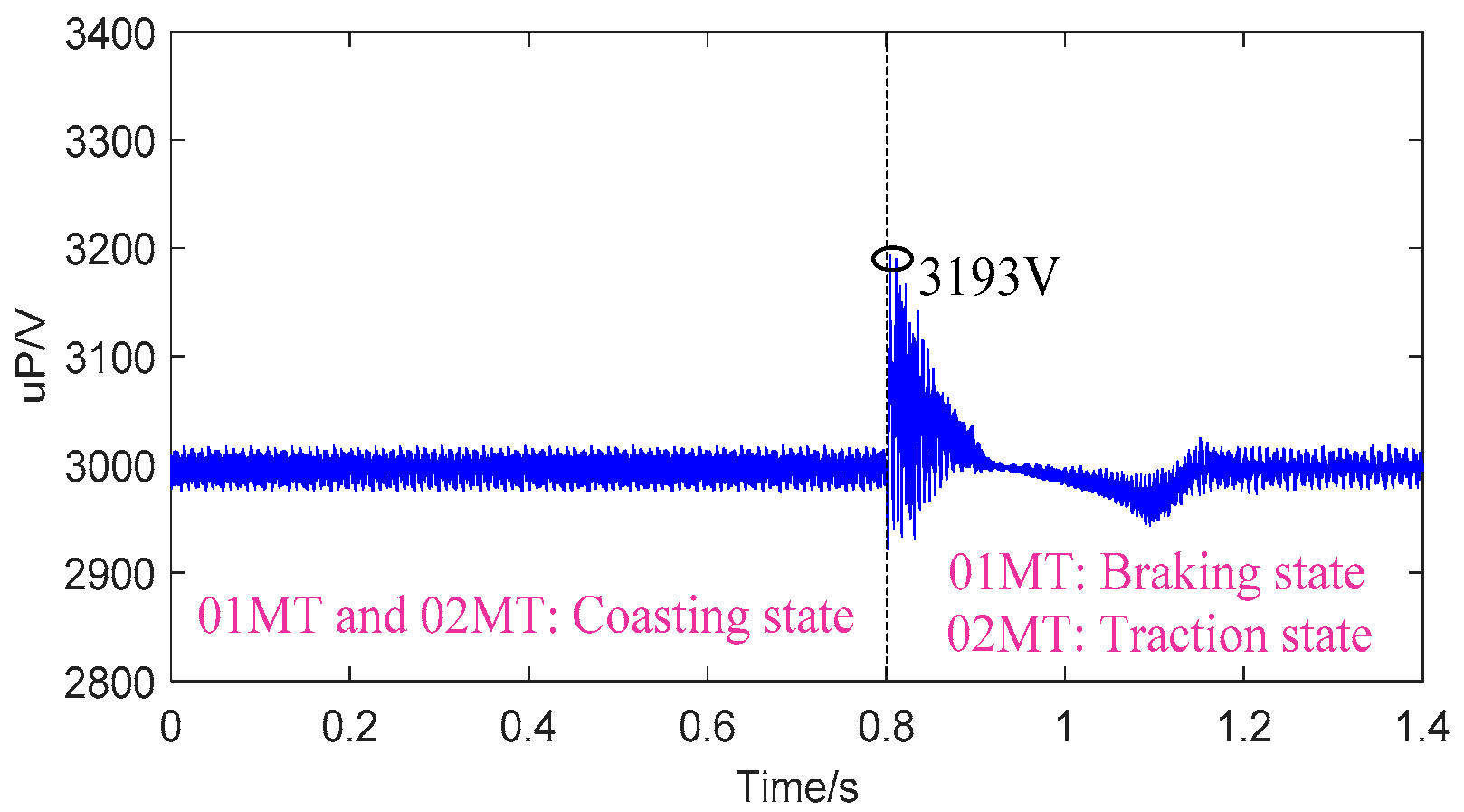
In case 1, 01 MT keeps coasting during 0~0.8 s and enters the RB state at 0.8 s, while 02 MT keeps coasting during 0~0.8 s but starts traction at 0.8 s. In case 2, the running states of 01 MT are similar to those of case 1, while 02 MT keeps coasting during 0~0.9 s and begins its traction at 0.9 s. In case 3, both of the two MTs are in their coasting states during 0~0.8 s and simultaneously start RB at 0.8 s.
4.2.1. Case 1
In Figure 19, before the RBEFS is introduced, the UPmax of 01 MT reaches 3193 V, i.e., ΔUP = 6.54% compared to the stable AVG amplitude before RB (2997 V). It does not reach the action threshold, U0 = 3360 V. Therefore, the voltage fluctuation stays the same with or without the RBEFS. By comparing Figure 16b and Figure 19, it can be observed that the voltage rise of 01 MT caused by RB is significantly offset by the simultaneous traction of 02 MT. The UPmax is reduced from 3850.1 V to 3193 V.
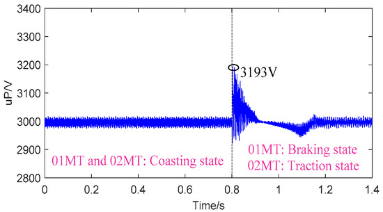
Figure 19.
PR voltage fluctuations of 01 MT with and without RBEFS in case 1.
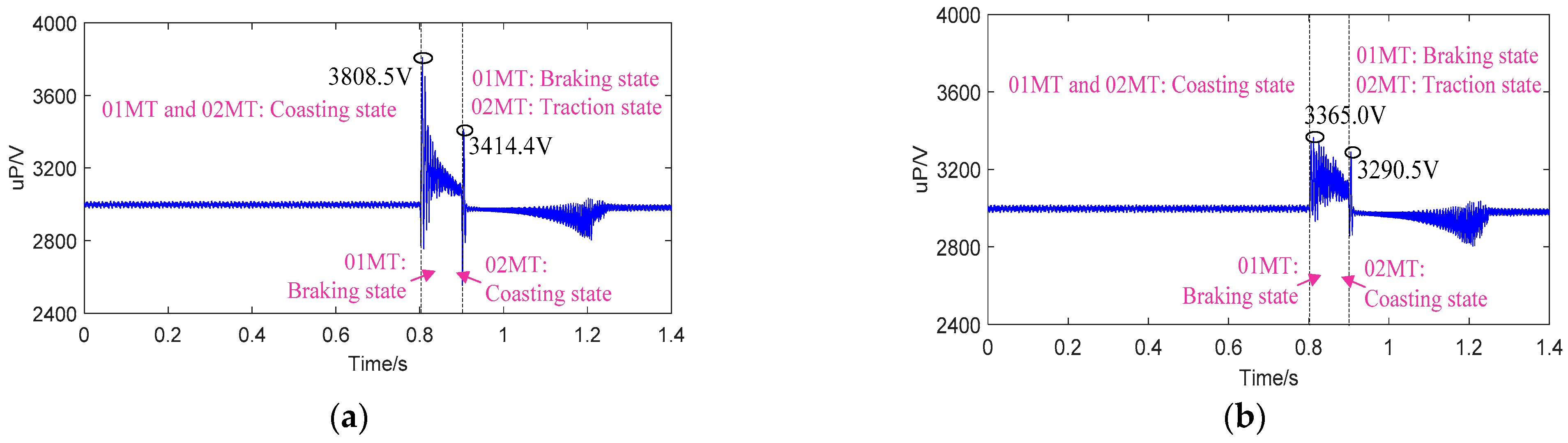
4.2.2. Case 2
RB energy can be utilized by a neighboring train that might be accelerating within the same power supply section as the braking one. However, this involves a high level of uncertainty since there is no guarantee that a train will be accelerating at the same time and in the right location when/where RB is available. Thus, the time-lapse scenario is analyzed.
As depicted in Figure 20, the severe voltage fluctuation firstly appears when 01 MT enters RB at 0.8 s, and it appears again when 02 MT begins traction at 0.9 s. Obviously, the peak value in the second occurrence is much lower than that in the first occurrence. Because both of the over-voltages (UPmax in order are 3808.5 V at 0.8 s and 3414.4 V at 0.9 s) exceed the action threshold value (U0 = 3360 V), the device action is carried out to restrain the two over-voltage peaks to 3365.0 V and 3290.5 V, respectively. It is observed in Table 4 that the inhibition percentage is positively related to the PR voltage rise. By comparing Figure 19 and Figure 20b, the time-lapse over-voltage offset is far lower than the simultaneous over-voltage offset.
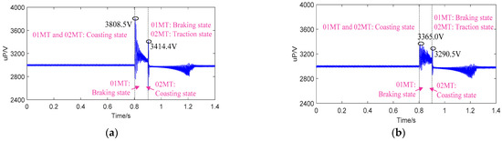
Figure 20.
PR voltage fluctuations in case 2: (a) with the RBEFS; (b) without the RBEFS.
Table 4.
Comparison of ΔUP of 01 MT during RB scenario in case 2.
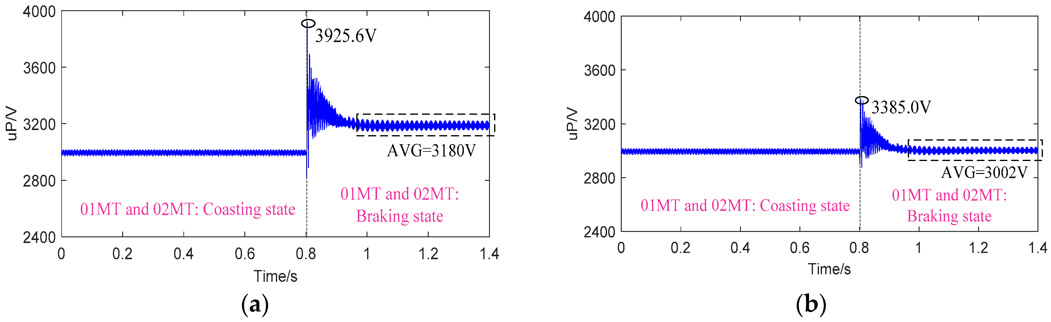
4.2.3. Case 3
By comparing Figure 16a and Figure 21a, the simultaneous entry of two trains into the RB status results in a more significant voltage rise, which is from 3850.1 V to 3925.6 V for the UPmax and from 3080 V to 3180 V for the stable AVG amplitudes during RB. This illustrates that the superimposed over-voltage effect caused by the simultaneous RB of the other MT is very significant. By comparing Table 2 and Table 5, the inhibition percentages of the UPmax and the stable AVG amplitudes without the effect of 02 MT are, in order, 15.80% and 2.37%, lower than those with the simultaneous RB effect (18.03% and 5.94%). This also proves that the inhibition percentage is positively related to the PR voltage rise.
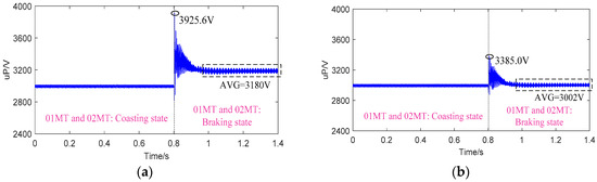
Figure 21.
PR voltage fluctuations in case 3: (a) with the RBEFS; (b) without the RBEFS.
Table 5.
Comparison of PR voltage rise percentages during RB scenario in case 3.
5. Conclusions
As an advancement to the previous literature, the PR voltage behavior and the effect of the RBEFS on the PR voltage rise inhibitions in the MLS maglev RB cases are studied. With a detailed consideration of the AC properties and energy dispersal path, the maglev electrical power model is built. Since the LIM air gap is different from the wheeled transport train motor and it results in different grid voltage rise behavior, the motor characteristics of the MLS motor are carefully incorporated in the vehicle model. The DC 3 kV traction voltage and 160~200 km/h train speed are taken into account and the influences of braking power, traction grid impedance and supply voltage level on the voltage fluctuations are investigated. The PR voltage fluctuations before and after putting the RBEFS into use are compared. The obtained results can be summarized as follows.
- (1)
- The higher MT speed and steeper downhill slope lead to the larger RB power and higher PR voltage rise, but the influence of the downhill slope gradient is relatively insignificant compared to that of the speed. The voltage flow direction along the line is different before and after RB. Higher traction grid impedance from the substation to the MT results in a higher instantaneous PR voltage rise and a lower stable PR voltage during RB. A higher traction voltage leads to a higher voltage rise.
- (2)
- The inhibition percentage of the RBEFS is positively related to the PR voltage rise. Therefore, since the increases in MT speed and traction voltage lead to the higher voltage rise, the voltage rise inhibition percentage keeps increasing with the MT speed and the traction voltage level both for the maximum value and the stable AVG amplitude during RB.
- (3)
- The offset for the PR voltage rise is very significant when two running trains on the same power supply section simultaneously enter the opposite state (traction state vs RB state). However, the offset amplitudes are notably lower when the offset moments of the two MTs are inconsistent by even only 0.1 s. The superimposed over-voltage effect is very significant when the other MT begins RB at the same time.
Based on the results of this paper, the vehicle–grid model can be further improved by considering the linear motor electrical structure when analyzing the influence of motor parameters on the RB over-voltages. The effects of the different inverter control approaches and other energy re-utilization applications, such as the super-capacitor energy storage device, will be the next focus to control the voltage rise.
Funding
This research was funded by the National Natural Science Foundation of China, grant number 52202450 and the Fundamental Research Funds for the Central Universities, grant numbers 22120220462 and 22120230110.
Data Availability Statement
The data are contained within this article.
Acknowledgments
The original parameters of the model in Figure 6 are provided by my affiliation (National Maglev Transportation Engineering R&D Center in Tongji University) and cooperative affiliation (CRRC Qingdao Sifang Locomotive and Rolling Stock Co., Ltd. (Qingdao, China) and Southwest Jiaotong University (Chengdu, China)).
Conflicts of Interest
The author declares no conflicts of interest.
References
- Lu, Q.; He, B.; Wu, M.; Zhang, Z.; Luo, J.; Zhang, Y.; He, R.; Wang, K. Establishment and analysis of energy consumption model of heavy-haul train on large long slope. Energies 2018, 11, 965. [Google Scholar] [CrossRef]
- Oliveira, R.; Mattos, L.S.; Ferreira, A.C.; Stephan, R.M. Regenerative braking of a linear induction motor used for the traction of a MagLev vehicle. In Proceedings of the Brazilian Power Electronics Conference, Gramado, Brazil, 27–31 October 2013; pp. 950–956. [Google Scholar]
- Demirci, I.E.; Celikoglu, H.B. Timetable optimization for utilization of regenerative braking energy: A single line case over Istanbul metro network. In Proceedings of the 21st International Conference on Intelligent Transportation Systems, Maui, HI, USA, 4–7 November 2018; pp. 2309–2314. [Google Scholar]
- Yildiz, A.; Arikan, O.; Keskin, K. Traction energy optimization considering comfort parameter: A case study in istanbul metro line. Electr. Power Syst. Res. 2023, 218, 4115–4130. [Google Scholar] [CrossRef]
- Hoo, D.S.; Chua, K.H.; Hau, L.C.; Chong, K.Y.; Lim, Y.S.; Chua, X.R.; Wang, L. An Investigation on recuperation of regenerative braking energy in DC railway electrification system. In Proceedings of the IEEE International Conference in Power Engineering Application, Shah Alam, Malaysia, 7–8 March 2022; pp. 1–6. [Google Scholar]
- Shiri, A.; Shoulaie, A.; Lesani, H. Design optimization and analysis of single-sided linear induction motor, considering all phenomena. IEEE Trans. Energy Convers. 2012, 27, 516–525. [Google Scholar] [CrossRef]
- Jefimowski, W.; Szelag, A. The multi-criteria optimization method for implementation of a regenerative inverter in a 3 kV DC traction system. Electr. Power Syst. Res. 2018, 161, 61–73. [Google Scholar] [CrossRef]
- Panda, N.K.; Poikilidis, M.; Nguyen, P.H. Cost-effective upgrade of the dutch traction power network: Moving to Bi-directional and controllable 3 kV DC substations for improved performance. IET Electr. Syst. Transp. 2023, 13, 1–13. [Google Scholar] [CrossRef]
- Menicanti, S.; Benedetto, M.D.; Lidozzi, A.; Solero, L.; Crescimbini, F. Recovery of train braking energy in 3 kV DC railway systems: A case of study. In Proceedings of the International Symposium on Power Electronics, Electrical Drives, Automation and Motion, Sorrento, Italy, 24–26 June 2020; pp. 1–6. [Google Scholar]
- Jefimowski, W.; Drarzek, Z. Distributed module-based power supply enhancement system for 3 kV DC traction. Energies 2023, 16, 401. [Google Scholar] [CrossRef]
- An, B.; Liu, S.; Liu, S. Simulation of ground rheostatic braking in mid-to-low speed maglev train. In Proceedings of the Chinese Control and Decision Conference, Changsha, China, 31 May 2014; pp. 4702–4706. [Google Scholar]
- Rigaut, T.; Carpentier, P.; Chancelier, J.P.; De Lara, M.; Waeytens, J. Stochastic Optimization of braking energy storage and ventilation in a subway station. IEEE Trans. Power Syst. 2019, 34, 1256–1263. [Google Scholar] [CrossRef]
- Ceraolo, M.; Lutzemberger, G.; Meli, E.; Pugi, L.; Rindi, A.; Pancari, G. Energy storage systems to exploit regenerative braking in DC railway systems: Different approaches to improve efficiency of modern high-speed trains. J. Energy Storage 2018, 16, 269–279. [Google Scholar] [CrossRef]
- Ghaviha, N.; Campillo, J.; Bohlin, M.; Dahlquist, E. Review of application of energy storage devices in railway transportation. Energy Procedia 2017, 105, 4561–4568. [Google Scholar] [CrossRef]
- Mayrink, S.; Oliveira, J.G.; Dias, B.H.; Oliveira, L.W.; Ochoa, J.S.; Rosseti, G.S. Regenerative braking for energy recovering in diesel-electric freight trains: A technical and economic evaluation. Energies 2020, 13, 963. [Google Scholar] [CrossRef]
- Khodaparastan, M. Recuperation of Regenerative Braking Energy in Electric Rail Transit Systems. Ph.D. Thesis, The City College of New York, New York, NY, USA, 2020. [Google Scholar]
- Almaksour, K.; Caron, H.; Kouassi, N.; Letrouvé, T.; Navarro, N.; Saudemont, C.; Robyns, B. Mutual impact of train regenerative braking and inverter based reversible DC railway substation. In Proceedings of the 21st European Conference on Power Electronics and Applications, Genova, Italy, 3–5 September 2019; pp. P.1–P.9. [Google Scholar]
- Lin, S.; Huang, D.; Wang, A.; Huang, Y.; Zhao, L.; Luo, R.; Lu, G. Research on the regeneration braking energy feedback system of urban rail transit. IEEE Trans. Veh. Technol. 2019, 68, 7329–7339. [Google Scholar] [CrossRef]
- Steiner, M.; Klohr, M.; Pagiela, S. Energy storage system with ultracaps on board of railway vehicles. In Proceedings of the European Conference on Power Electronics and Applications, Aalborg, Denmark, 4 January 2007; pp. 1–10. [Google Scholar]
- Zhang, Q.; Zhang, Y.; Huang, K.; Tasiu, I.A.; Lu, B.; Meng, X.; Liu, Z.; Sun, W. Modeling of regenerative braking energy for electric multiple units passing long downhill section. IEEE Trans. Transp. Electrif. 2022, 8, 3742–3758. [Google Scholar] [CrossRef]
- Rufer, A.; Hotellier, D.; Barrade, P. A supercapacitor-based energy storage substation for voltage compensation in weak transportation networks. IEEE Trans. Power Deliv. 2004, 19, 629–636. [Google Scholar] [CrossRef]
- Suárez, M.A.; González, J.W.; Celis, I. Transient overvoltages in a railway system during braking. In Proceedings of the IEEE/PES Transmission and Distribution Conference and Exposition: Latin America, Sao Paulo, Brazil, 8–10 November 2010; pp. 204–211. [Google Scholar]
- Ebrahimian, A.; Dastfan, A.; Ahmadi, S. Metro train line voltage control: Using average modeling bidirectional DC-DC converter. In Proceedings of the 9th Annual Power Electronics, Drives Systems and Technologies Conference, Tehran, Iran, 13–15 February 2018; pp. 7–13. [Google Scholar]
- Li, Y.; Zhang, H.; Bu, L.; Liu, W.; Zhang, J.; Wu, T. Discussion of the energy-saving effect of inverter feedback devices from energy consumption of traveling trains. J. Railw. Sci. Eng. 2020, 17, 2381–2386. [Google Scholar]
- Zhou, Y.; Wu, S.; Wei, J.; Kong, Q. Analysis of energy feed system of metro under adaptive moment of inertia VSG control. In Proceedings of the 15th IEEE Conference on Industrial Electronics and Applications, Kristiansand, Norway, 9–13 November 2020; pp. 726–731. [Google Scholar]
- Li, S.; Wu, S.; Xiang, S.; Zhang, Y.; Guerrero, J.M.; Vasquez, J.C. Research on synchronverter-based regenerative braking energy feedback system of urban rail transit. Energies 2020, 13, 4418. [Google Scholar] [CrossRef]
- Krim, Y.; Almaksour, K.; Caron, H.; Letrouvé, T.; Saudemont, C.; Francois, B.; Robyns, B. Comparative study of two control techniques of regenerative braking power recovering inverter based DC railway substation. In Proceedings of the 22nd European Conference on Power Electronics and Applications, Lyon, France, 7–11 September 2020; pp. 1–9. [Google Scholar]
- Liang, H.; Li, P. The supercapacitor energy storage system is applied to Shanghai medium-low speed maglev train test line. In Proceedings of the International Conference on Sensing, Measurement & Data Analytics in the era of Artificial Intelligence, Nanjing, China, 21–23 October 2021; pp. 1–6. [Google Scholar]
- Huang, K.; Lin, G.; Liu, Z. Prediction approach of negative rail potentials and stray currents in medium-low-speed maglev. IEEE Trans. Transp. Electrif. 2022, 8, 3801–3815. [Google Scholar] [CrossRef]
- Xu, J.; Chen, C.; Sun, Y.; Rong, L.; Lin, G. Nonlinear dynamic characteristic modeling and adaptive control of low speed maglev train. Int. J. Appl. Electromagn. Mech. 2020, 62, 73–92. [Google Scholar] [CrossRef]
- Isfahani, A.H.; Ebrahimi, B.M.; Lesani, H. Design optimization of a low-speed single-sided linear induction motor for improved efficiency and power factor. IEEE Trans. Magn. 2008, 44, 266–272. [Google Scholar] [CrossRef]


Disclaimer/Publisher’s Note: The statements, opinions and data contained in all publications are solely those of the individual author(s) and contributor(s) and not of MDPI and/or the editor(s). MDPI and/or the editor(s) disclaim responsibility for any injury to people or property resulting from any ideas, methods, instructions or products referred to in the content. |
© 2024 by the author. Licensee MDPI, Basel, Switzerland. This article is an open access article distributed under the terms and conditions of the Creative Commons Attribution (CC BY) license (https://creativecommons.org/licenses/by/4.0/).