
Enhanced Forecasting Accuracy of a Grid-Connected Photovoltaic Power Plant: A Novel Approach Using Hybrid Variational Mode Decomposition and a CNN-LSTM Model


Abstract
1. Introduction
- Proposing a novel hybrid model combining the VMD algorithm with the CNN-LSTM architecture for PV power forecasting, marking the first initiative to explore such a hybrid model for these specific tasks.
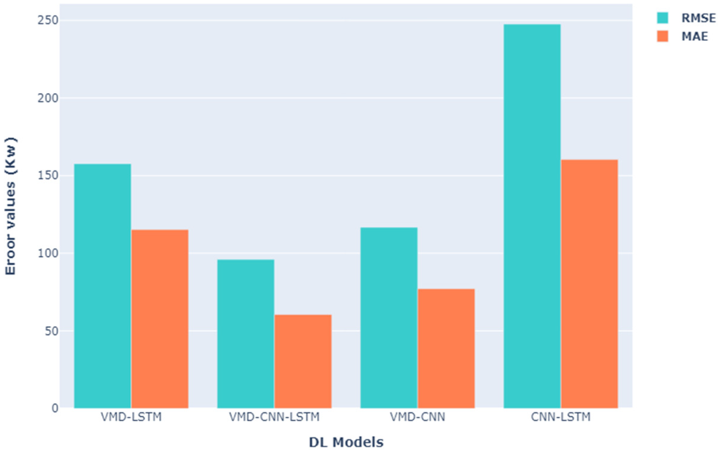
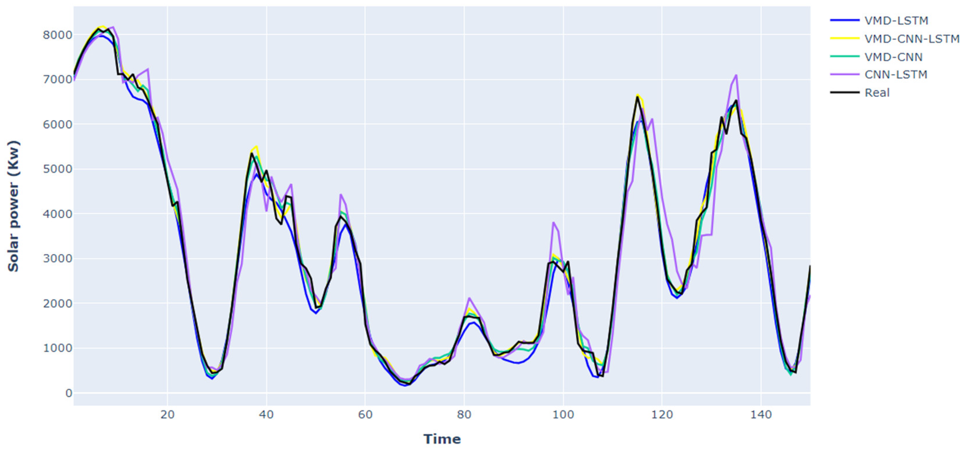
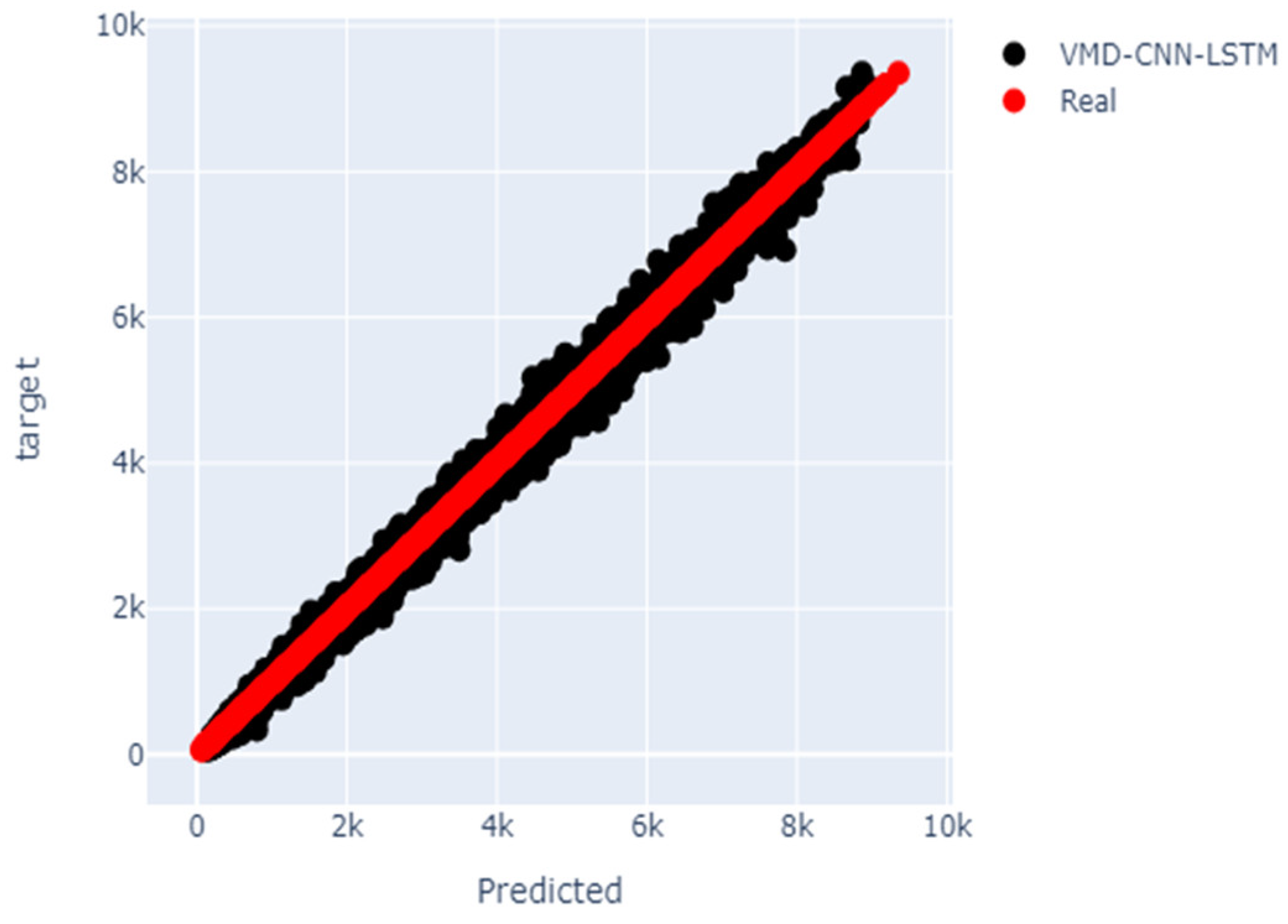
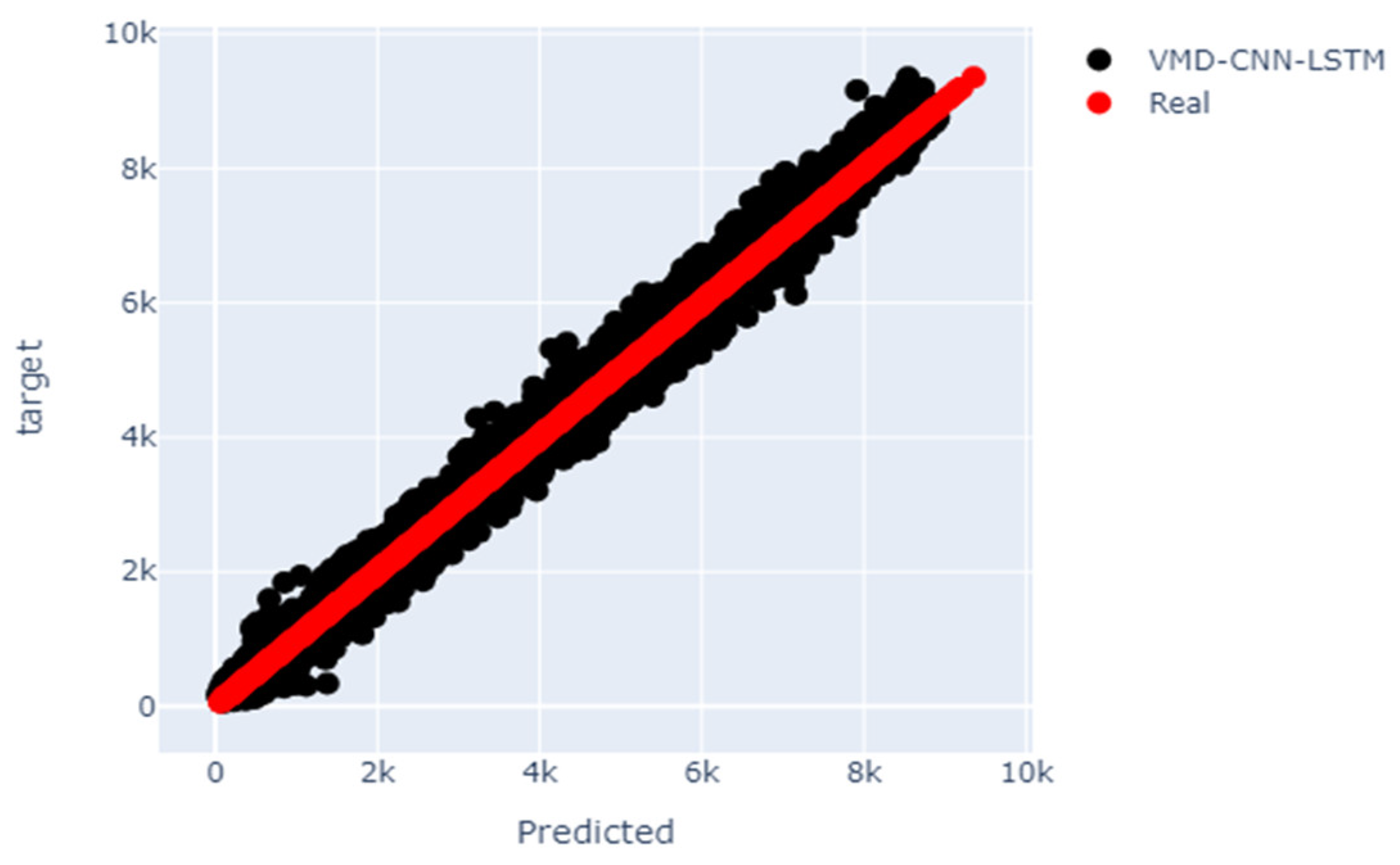
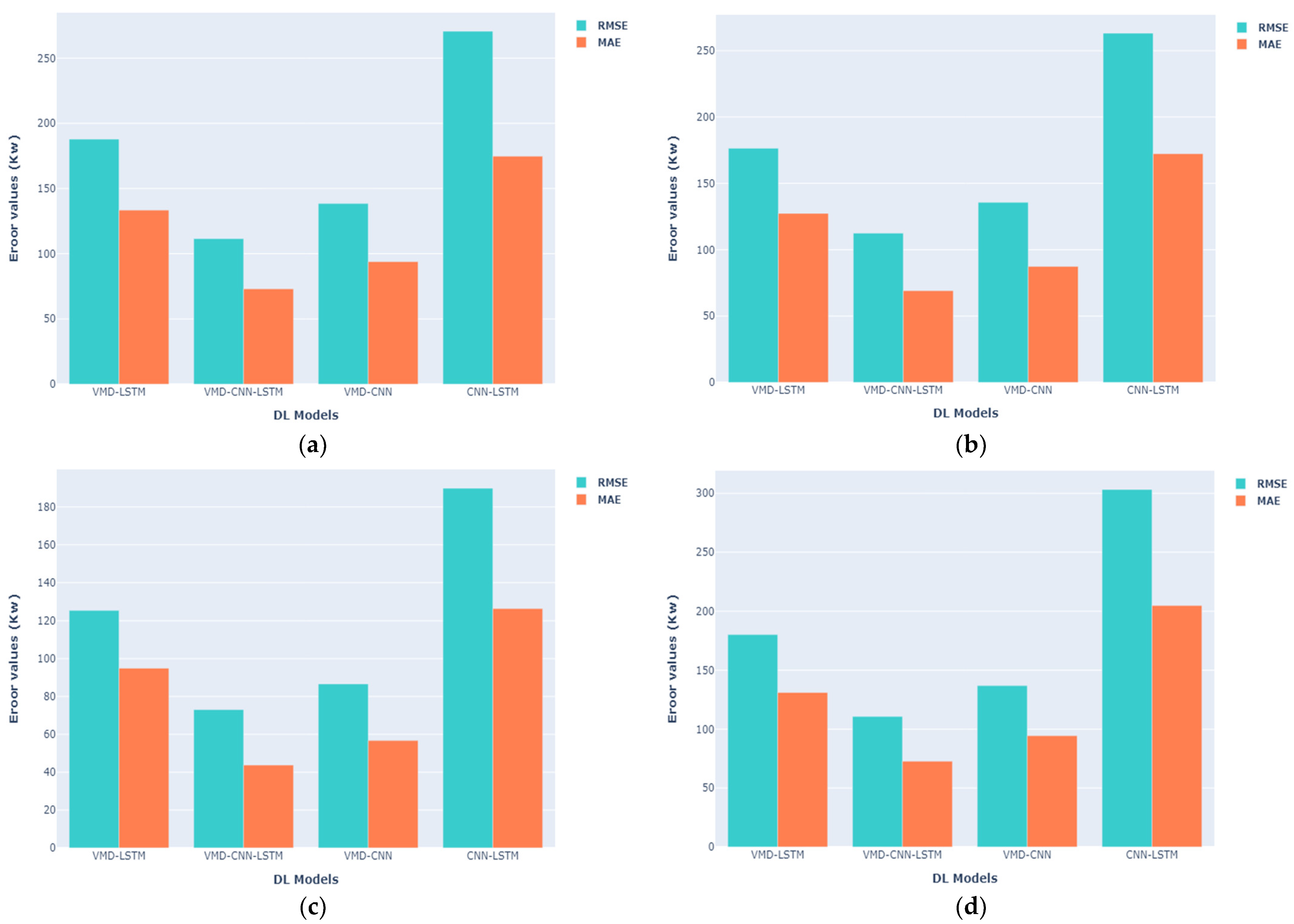
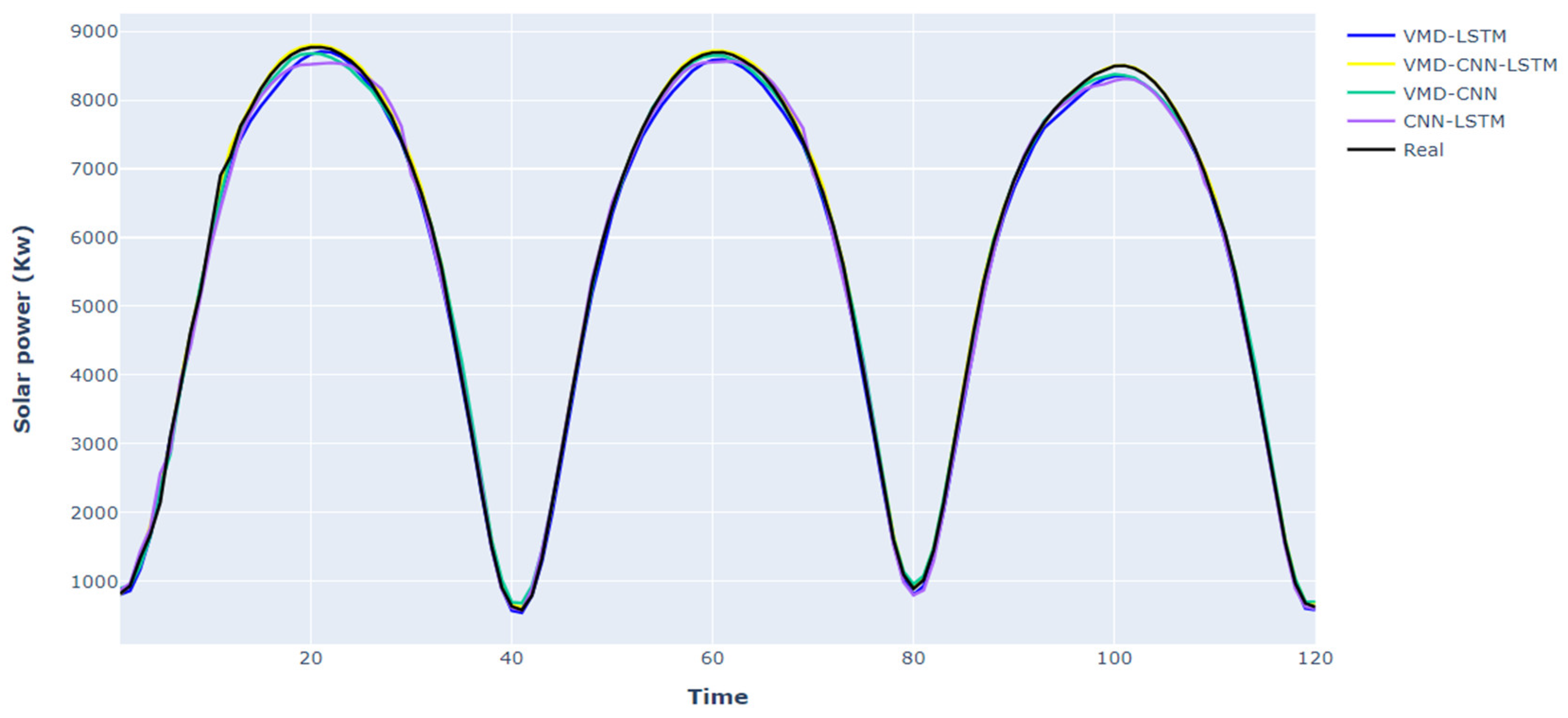
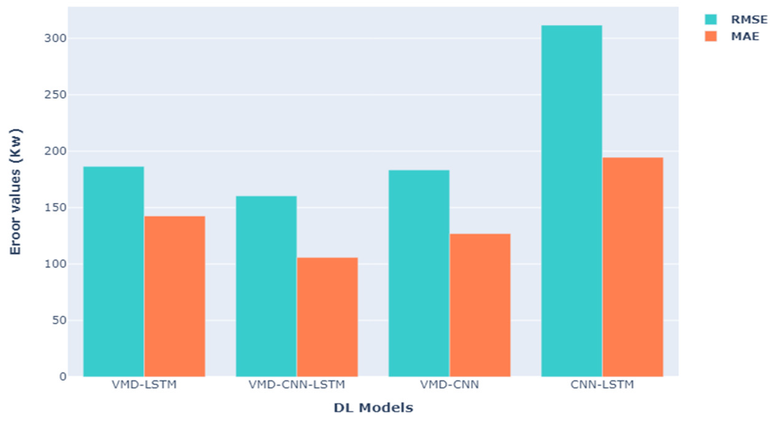
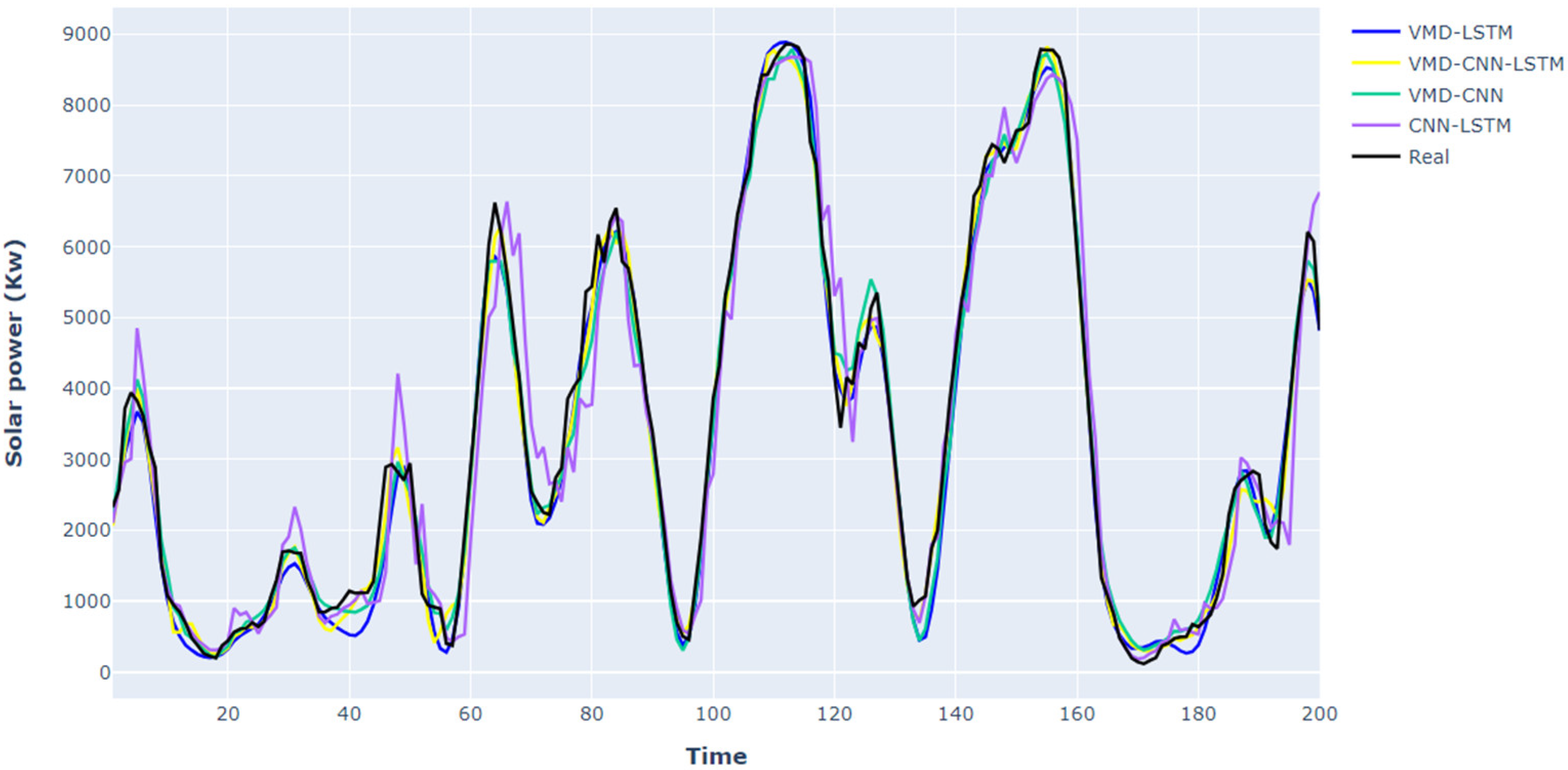
- Conducting a comparative analysis against various DL models, including VMD-CNN, VMD-LSTM, and CNN-LSTM, to assess the precision and performance enhancement attributed to the unique integration of CNN, LSTM, and VMD components.
- Effectively utilizing actual data from the solar PV farm, ensuring the practical applicability of our forecasting approach to real-world applications in energy management systems.
2. Literature Review
3. Materials and Methods
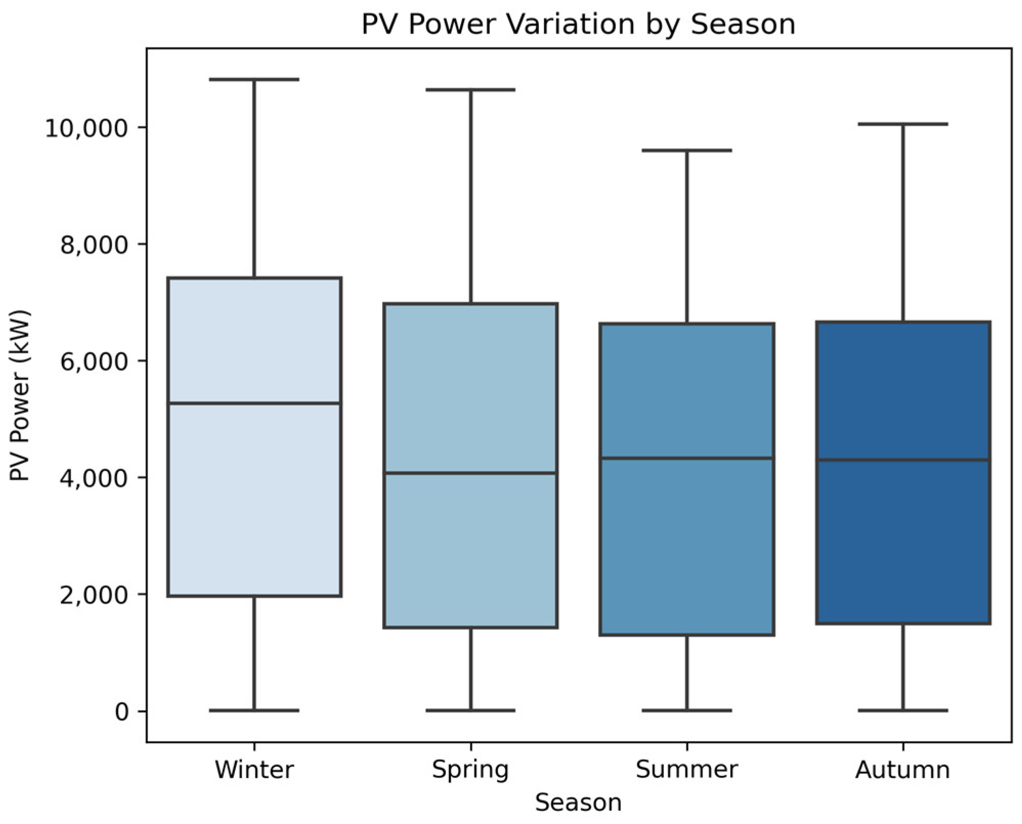
3.1. Data Collection
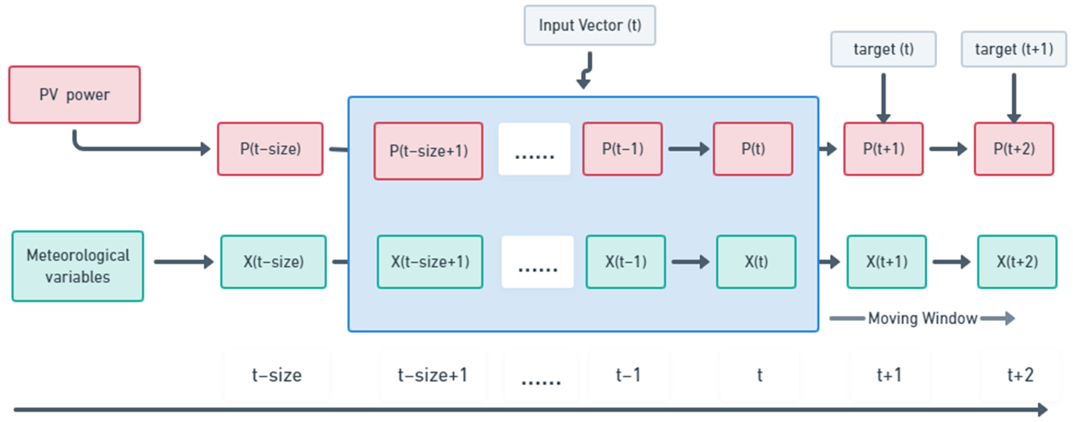
3.2. Data Processing
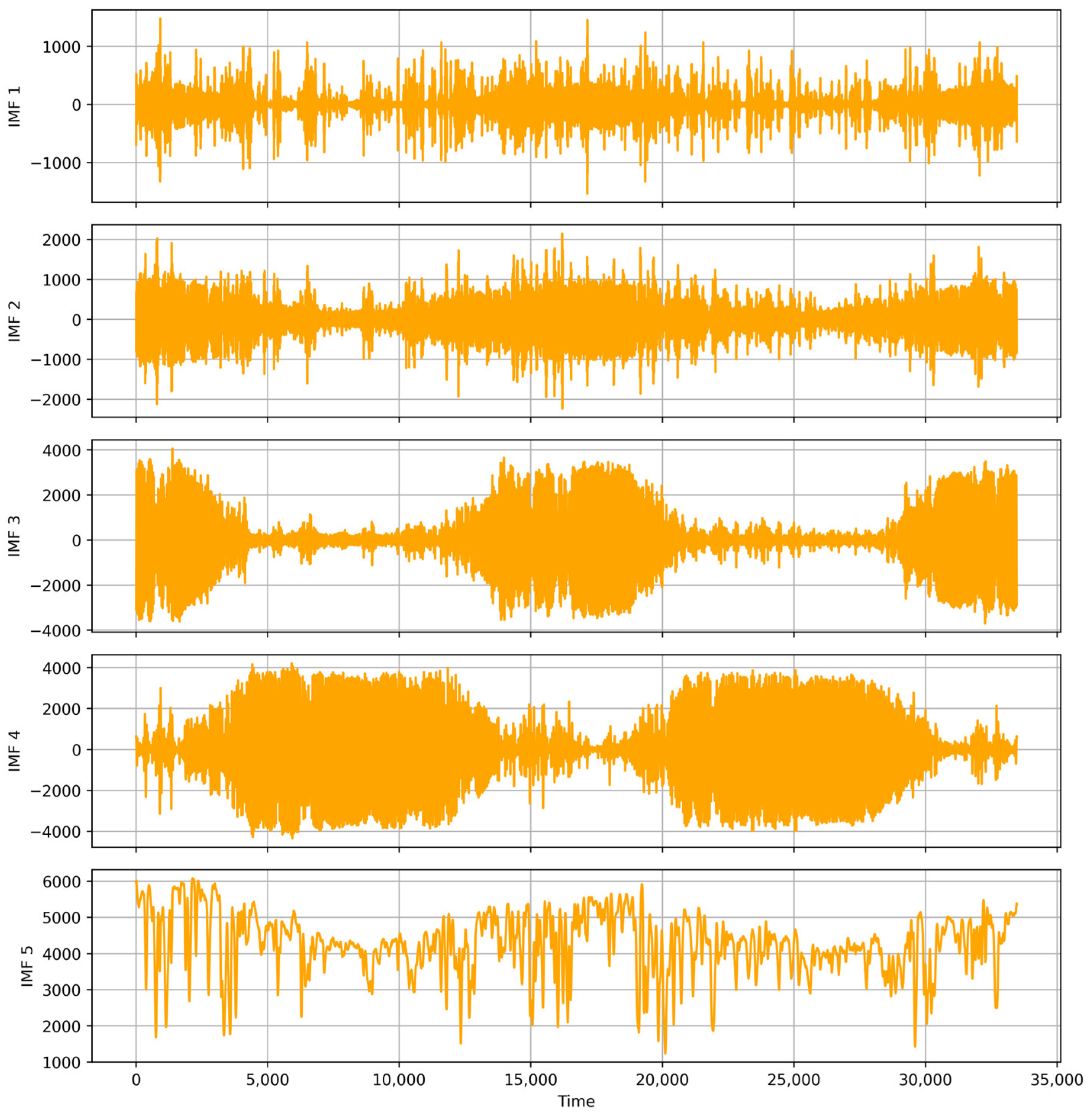
3.3. Variational Mode Decomposition (VMD)
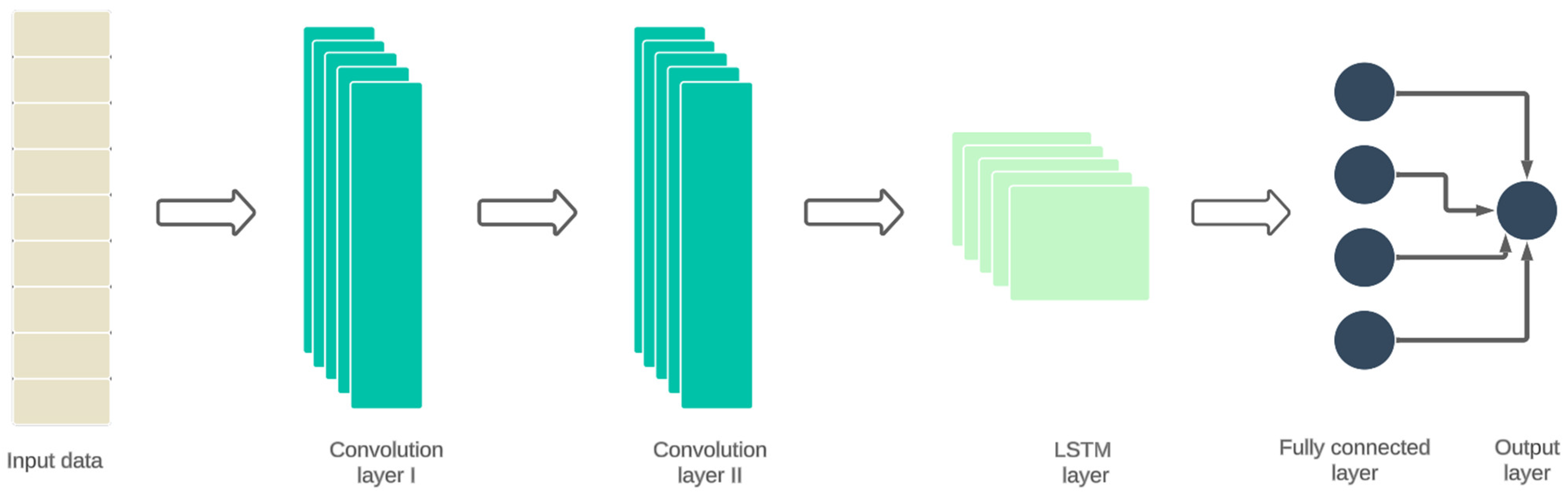
3.4. Convolutional Neural Network–Long Short-Term Memory (CNN-LSTM)
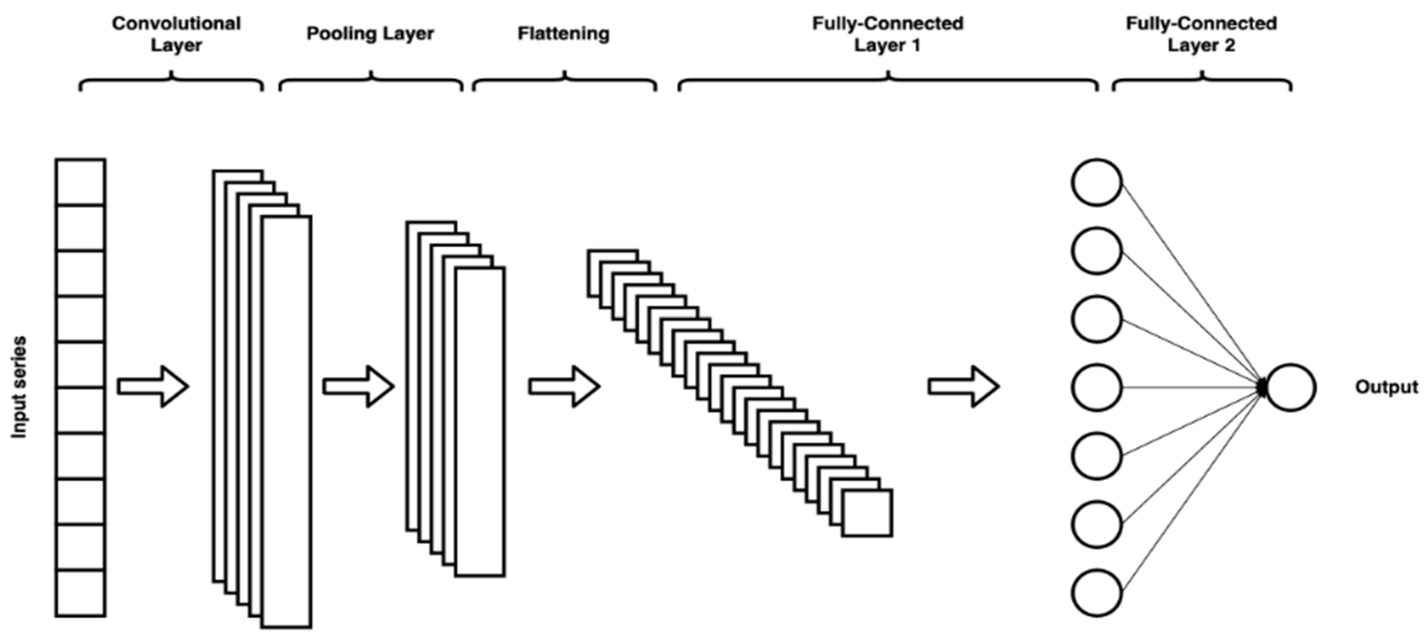
3.4.1. Convolutional Neural Network (CNN)
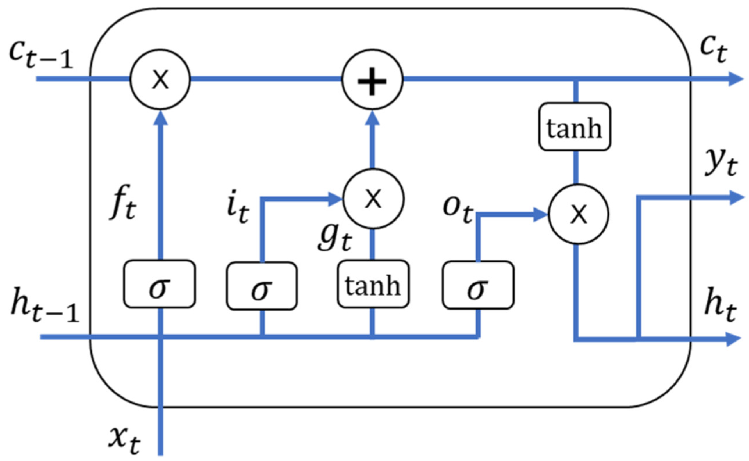
3.4.2. Long Short-Term Memory (LSTM)
- The input gate controls which parts of the new information will be stored in the cell state.
- The forget gate controls which parts of the cell state will be thrown away.
- The output gate computes the cell’s output and sends it to the next cell in the chain.
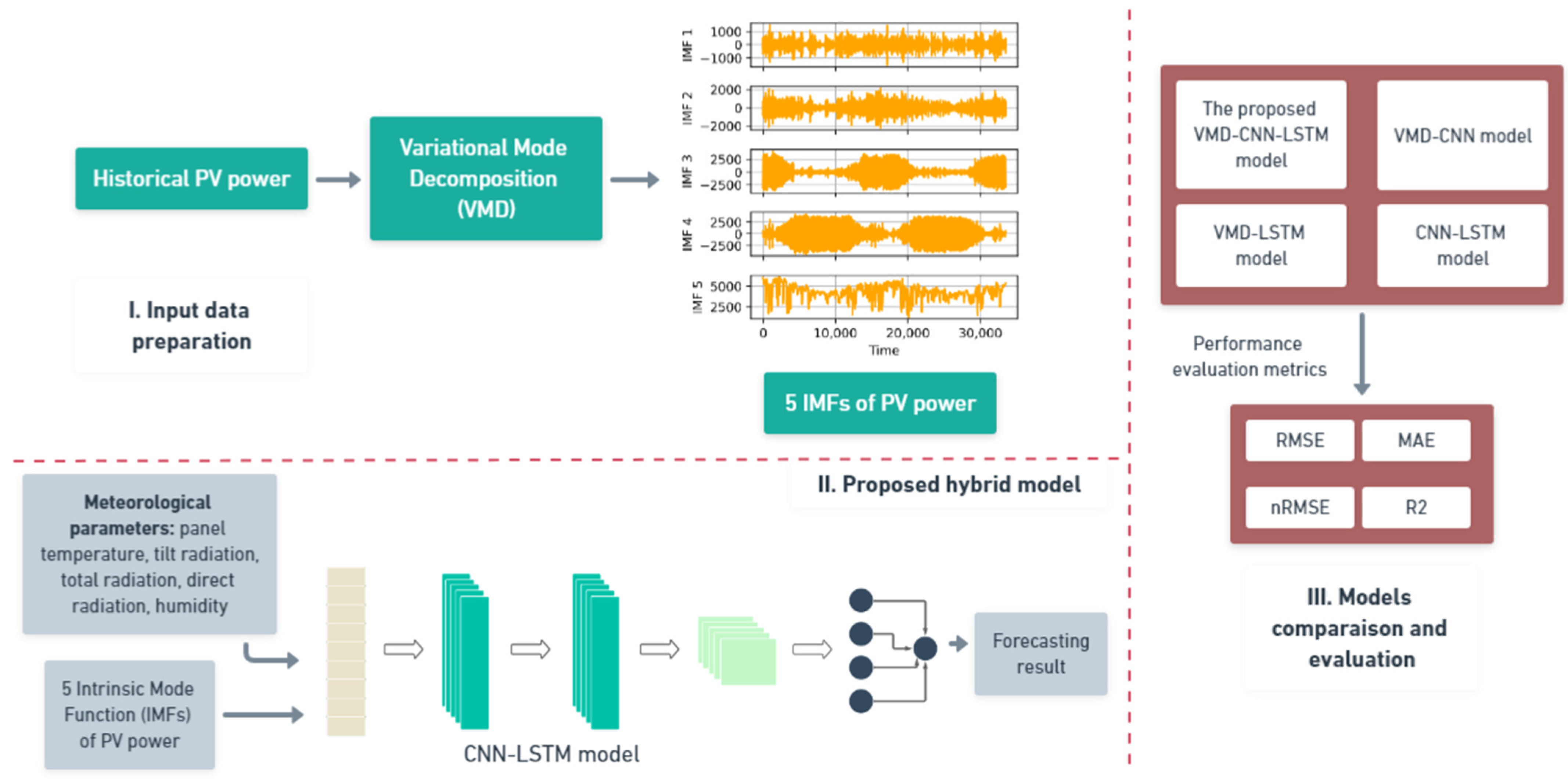
3.5. Framework of the Proposed Method
4. Case Study
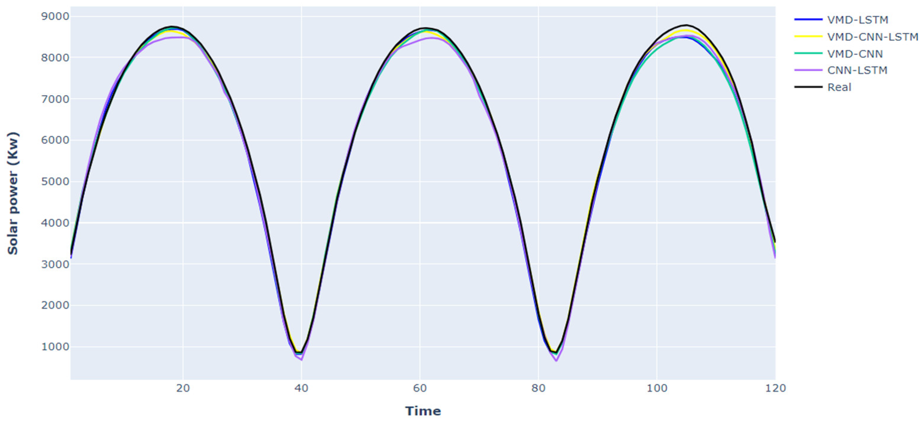
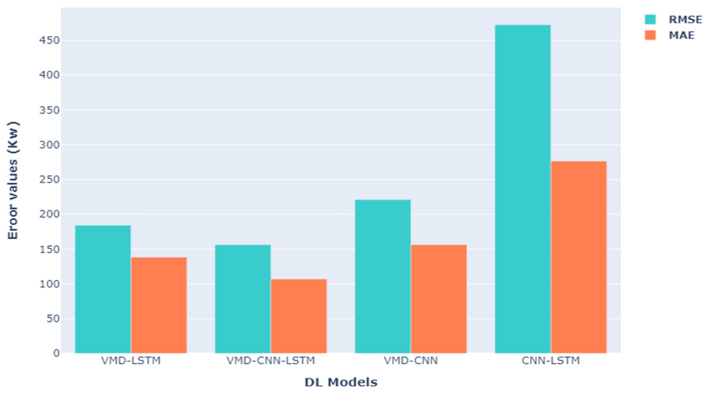
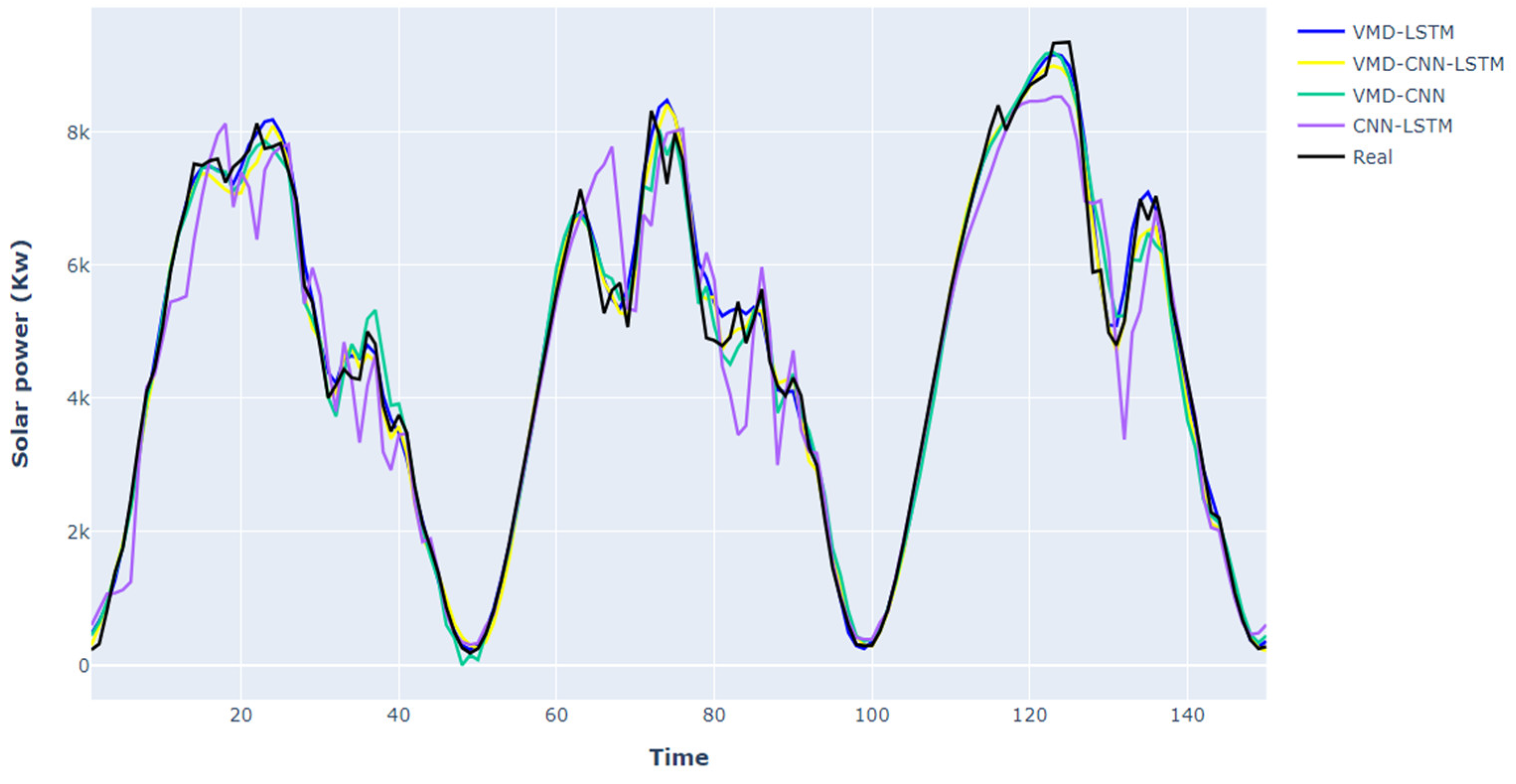
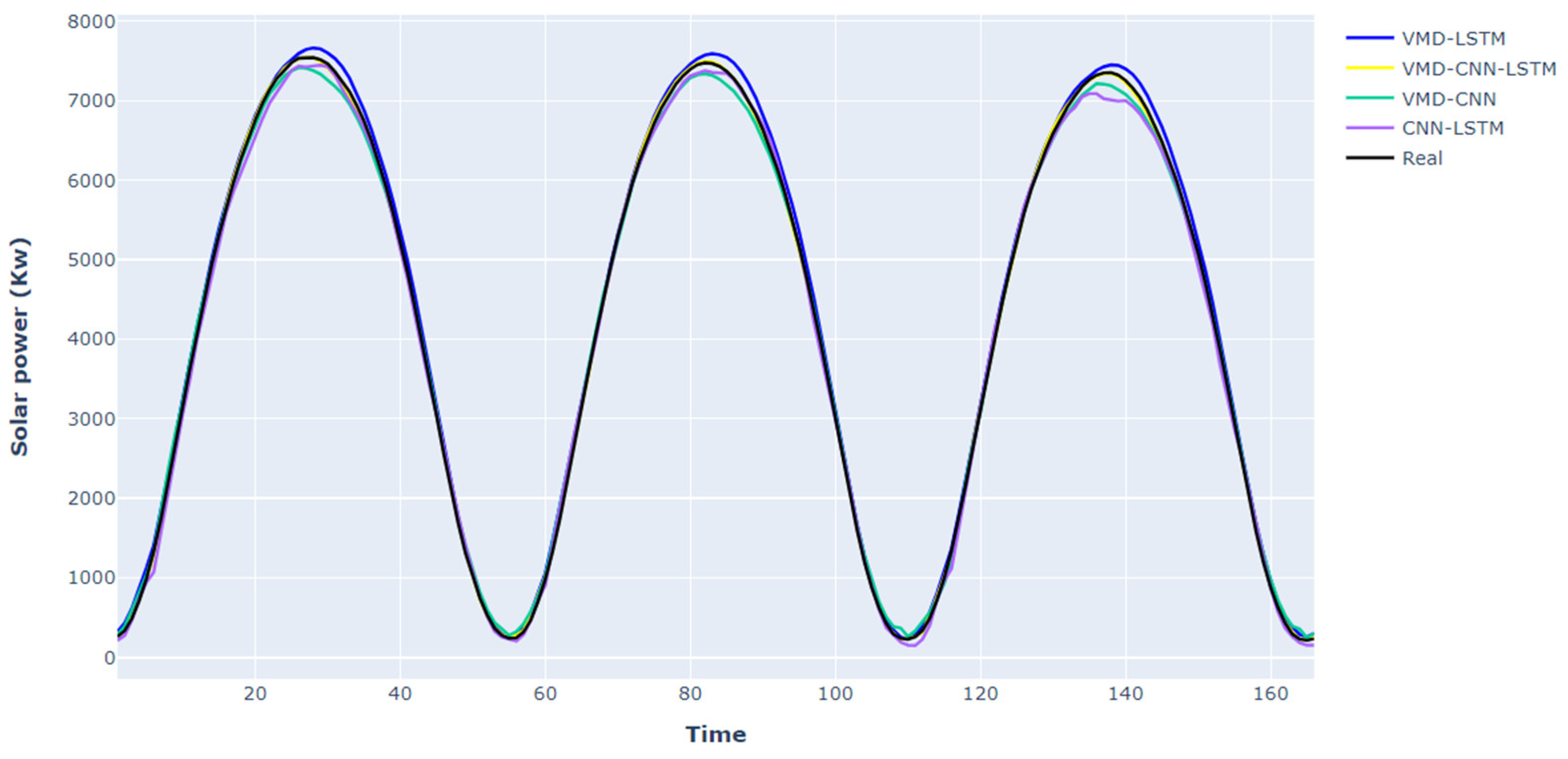
Experimental Studies and Results
- VMD preprocessing: VMD is adept at extracting intrinsic modes in data. This becomes especially important in solar energy predictions, where the input signals can be nonstationary or possess multiple modalities. VMD simplifies the task for the subsequent layers by addressing such complexities during preprocessing.
- The 1D-CNN advantage: 1D-CNNs are fine-tuned for handling sequential data, perfectly aligning with the time series nature of data. Their expertise rests in efficiently identifying specific temporal trends. In solar energy prediction, capturing short-term patterns, such as variations in solar irradiance, becomes pivotal.
- The LSTM advantage: While LSTM models are widely recognized for effectively retaining and utilizing information related to long-term dependencies, their real strength is their proficiency in modeling sequential data. Even for short-term forecasts, the ability of LSTMs to incorporate information from previous time steps can be useful. They capture the flow of data, which can be crucial for solar forecasts.
- The hybrid approach: The integration of VMD, 1D-CNN, and LSTM techniques allows their respective functionalities to be combined into a unified methodology. With the complexity simplified by VMD, 1D-CNN identification of local patterns, and LSTM’s ability to incorporate information from past time steps, the model can address the diverse challenges inherent in solar forecasting.
5. Conclusions
- Investing in more robust data collection methods, including diverse metrological conditions and geographic locations, can improve model accuracy and applicability.
- Practical incorporation into an existing energy management system by addressing real-world challenges such as variable data flows, system integration complexities, and operational constraints.
Author Contributions
Funding
Data Availability Statement
Conflicts of Interest
References
- Singh, S.; Ranjan, V.; Tripathy, P.; Nachappa, M.N. Balanced load frequency control: Customized world cup algorithm—Driven pid optimization for two area power systems. Proc. Eng. Sci. 2024, 5, 331–342. [Google Scholar] [CrossRef]
- Meliani, M.; Barkany, A.E.; Abbassi, I.E.; Darcherif, A.M.; Mahmoudi, M. Energy management in the smart grid: State-of-the-art and future trends. Int. J. Eng. Bus. Manag. 2021, 13, 18479790211032920. [Google Scholar] [CrossRef]
- Aldosari, O.; Batiyah, S.; Elbashir, M.; Alhosaini, W.; Kanagaraj, N. Performance Evaluation of Multiple Machine Learning Models in Predicting Power Generation for a Grid-Connected 300 MW Solar Farm. Energies 2024, 17, 525. [Google Scholar] [CrossRef]
- Demir, V.; Citakoglu, H. Forecasting of solar radiation using different machine learning approaches. Neural Comput. Appl. 2023, 35, 887–906. [Google Scholar] [CrossRef]
- Boucetta, L.N.; Amrane, Y.; Arezki, S. Comparative Analysis of LSTM, GRU, and MLP Neural Networks for Short-Term Solar Power Forecasting. In Proceedings of the 2023 International Conference on Electrical Engineering and Advanced Technology (ICEEAT), Batna, Algeria, 5–7 November 2023; pp. 1–6. [Google Scholar] [CrossRef]
- Rai, A.; Shrivastava, A.; Jana, K.C. A robust auto encoder-gated recurrent unit (AE-GRU) based deep learning approach for short term solar power forecasting. Optik 2022, 252, 168515. [Google Scholar] [CrossRef]
- Liu, C.H.; Gu, J.C.; Yang, M.T. A simplified LSTM neural networks for one day-ahead solar power forecasting. IEEE Access 2021, 9, 17174–17195. [Google Scholar] [CrossRef]
- Akhter, M.N.; Mekhilef, S.; Mokhlis, H.; Almohaimeed, Z.M.; Muhammad, M.A.; Khairuddin, A.S.M.; Akram, R.; Hussain, M.M. An Hour-Ahead PV Power Forecasting Method Based on an RNN-LSTM Model for Three Different PV Plants. Energies 2022, 15, 6. [Google Scholar] [CrossRef]
- Suresh, V.; Aksan, F.; Janik, P.; Sikorski, T.; Revathi, B.S. Probabilistic LSTM-Autoencoder Based Hour-Ahead Solar Power Forecasting Model for Intra-Day Electricity Market Participation: A Polish Case Study. IEEE Access 2022, 10, 110628–110638. [Google Scholar] [CrossRef]
- Hu, Z.; Gao, Y.; Ji, S.; Mae, M.; Imaizumi, T. Improved multistep ahead photovoltaic power prediction model based on LSTM and self-attention with weather forecast data. Appl. Energy 2024, 359, 122709. [Google Scholar] [CrossRef]
- Suresh, V.; Janik, P.; Rezmer, J.; Leonowicz, Z. Forecasting solar PV output using convolutional neural networks with a sliding window algorithm. Energies 2020, 13, 723. [Google Scholar] [CrossRef]
- Feng, C.; Zhang, J. SolarNet: A sky image-based deep convolutional neural network for intra-hour solar forecasting. Sol. Energy 2020, 204, 71–78. [Google Scholar] [CrossRef]
- Heo, J.; Song, K.; Han, S.; Lee, D.-E. Multi-channel convolutional neural network for integration of meteorological and geographical features in solar power forecasting. Appl. Energy 2021, 295, 117083. [Google Scholar] [CrossRef]
- Rabehi, A.; Guermoui, M.; Lalmi, D. Hybrid models for global solar radiation prediction: A case study. Int. J. Ambient Energy 2020, 41, 31–40. [Google Scholar] [CrossRef]
- Moreira, M.O.; Balestrassi, P.P.; Paiva, A.P.; Ribeiro, P.F.; Bonatto, B.D. Design of experiments using artificial neural network ensemble for photovoltaic generation forecasting. Renew. Sustain. Energy Rev. 2021, 135, 110450. [Google Scholar] [CrossRef]
- Jebli, I.; Belouadha, F.-Z.; Kabbaj, M.I.; Tilioua, A. Prediction of solar energy guided by pearson correlation using machine learning. Energy 2021, 224, 120109. [Google Scholar] [CrossRef]
- Hochreiter, S. The vanishing gradient problem during learning recurrent neural nets and problem solutions. Int. J. Uncertain. Fuzziness Knowl. Based Syst. 1998, 6, 107–116. [Google Scholar] [CrossRef]
- Agga, A.; Abbou, A.; Labbadi, M.; El Houm, Y.; Ali, I.H.O. CNN-LSTM: An efficient hybrid deep learning architecture for predicting short-term photovoltaic power production. Electr. Power Syst. Res. 2022, 208, 107908. [Google Scholar] [CrossRef]
- Agga, A.; Abbou, A.; Labbadi, M.; El Houm, Y. Short-term self-consumption PV plant power production forecasts based on hybrid CNN-LSTM, ConvLSTM models. Renew. Energy 2021, 177, 101–112. [Google Scholar] [CrossRef]
- Alharkan, H.; Habib, S.; Islam, M. Solar Power Prediction Using Dual Stream CNN-LSTM Architecture. Sensors 2023, 23, 2. [Google Scholar] [CrossRef] [PubMed]
- Abou Houran, M.; Salman Bukhari, S.M.; Zafar, M.H.; Mansoor, M.; Chen, W. COA-CNN-LSTM: Coati optimization algorithm-based hybrid deep learning model for PV/wind power forecasting in smart grid applications. Appl. Energy 2023, 349, 121638. [Google Scholar] [CrossRef]
- Phan, Q.-T.; Wu, Y.-K.; Phan, Q.-D. An Approach Using Transformer-based Model for Short-term PV generation forecasting. In Proceedings of the 2022 8th International Conference on Applied System Innovation (ICASI), Nantou, Taiwan, 22–23 April 2022; pp. 17–20. [Google Scholar] [CrossRef]
- López Santos, M.; García-Santiago, X.; Echevarría Camarero, F.; Blázquez Gil, G.; Carrasco Ortega, P. Application of Temporal Fusion Transformer for Day-Ahead PV Power Forecasting. Energies 2022, 15, 14. [Google Scholar] [CrossRef]
- Wu, Z.; Pan, F.; Li, D.; He, H.; Zhang, T.; Yang, S. Prediction of Photovoltaic Power by the Informer Model Based on Convolutional Neural Network. Sustainability 2022, 14, 20. [Google Scholar] [CrossRef]
- Huang, N.E.; Shen, Z.; Long, S.R.; Wu, M.C.; Shih, H.H.; Zheng, Q.; Liu, H.H. The empirical mode decomposition and the Hilbert spectrum for nonlinear and non-stationary time series analysis. Proc. R. Soc. Lond. Ser. A Math. Phys. Eng. Sci. 1998, 454, 903–995. [Google Scholar] [CrossRef]
- Dragomiretskiy, K.; Zosso, D. Variational mode decomposition. IEEE Trans. Signal Process. 2013, 62, 531–544. [Google Scholar] [CrossRef]
- Taye, M.M. Theoretical understanding of convolutional neural network: Concepts, architectures, applications, future directions. Computation 2023, 11, 52. [Google Scholar] [CrossRef]
- Joseph, L.P.; Deo, R.C.; Prasad, R.; Salcedo-Sanz, S.; Raj, N.; Soar, J. Near real-time wind speed forecast model with bidirectional LSTM networks. Renew. Energy 2023, 204, 39–58. [Google Scholar] [CrossRef]
- Rahimi, N.; Park, S.; Choi, W.; Oh, B.; Kim, S.; Cho, Y.; Ahn, S.; Chong, C.; Kim, D.; Jin, C.; et al. A Comprehensive Review on Ensemble Solar Power Forecasting Algorithms. J. Electr. Eng. Technol. 2023, 18, 719–733. [Google Scholar] [CrossRef] [PubMed]
- Chicco, D.; Warrens, M.J.; Jurman, G. The coefficient of determination R-squared is more informative than SMAPE, MAE, MAPE, MSE and RMSE in regression analysis evaluation. PeerJ Comput. Sci. 2021, 7, e623. [Google Scholar] [CrossRef] [PubMed]


| Parameters | Values Range |
|---|---|
| Panel temperature (°C) | 1.70–71.70 |
| Tilt radiation (W/m2) | 0.0–1651.20 |
| Total radiation (W/m2) | 0.0–1387.20 |
| Direct radiation (W/m2) | 0.0–1365.60 |
| Humidity (%) | 0.10–74.80 |
| PV power (kW) | 0.0–10,815.0 |
| Forecasting Time Horizon | Models | Metrics | |||
|---|---|---|---|---|---|
| RMSE (kW) | MAE (kW) | nRMSE (%) | R2 (%) | ||
| 15 min ahead | VMD-LSTM | 157.62 | 115.26 | 3.7 | 99.2 |
| VMD-CNN | 116.68 | 77.12 | 2.7 | 99.7 | |
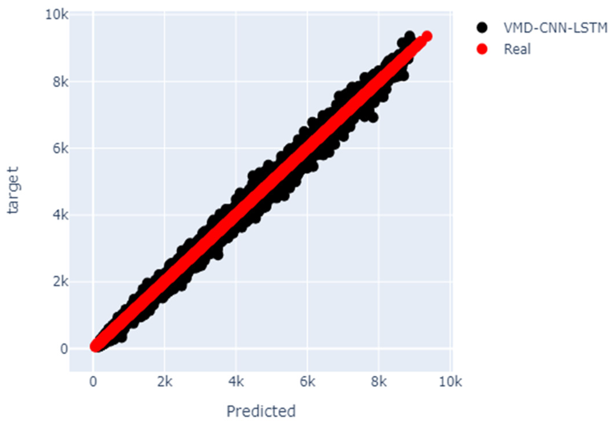
| VMD-CNN-LSTM | 96.04 | 60.50 | 2.2 | 99.8 | |
| CNN-LSTM | 247.61 | 160.36 | 5.9 | 99.0 | |
| 30 min ahead | VMD-LSTM | 186.52 | 142.54 | 4.5 | 99.4 |
| VMD-CNN | 183.35 | 126.89 | 4.3 | 99.5 | |
| VMD-CNN-LSTM | 160.31 | 105.80 | 3.8 | 99.6 | |
| CNN-LSTM | 311.66 | 194.55 | 7.4 | 98.5 | |
| 60 min ahead | VMD-LSTM | 184.20 | 138.29 | 4.4 | 99.4 |
| VMD-CNN | 221.12 | 156.26 | 5.2 | 99.2 | |
| VMD-CNN-LSTM | 160.31 | 115.17 | 3.7 | 99.6 | |
| CNN-LSTM | 472.40 | 276.41 | 11.3 | 96.6 | |
| Deep Learning Models | Prediction Time (s) | Model Complexity |
|---|---|---|
| VMD-LSTM | 0.68 | 172,929 parameters |
| VMD-CNN | 0.11 | 224,545 parameters |
| VMD-CNN-LSTM | 0.50 | 80,977 parameters |
| CNN-LSTM | 0.41 | 130,897 parameters |
| Season | Models | Metrics | ||
|---|---|---|---|---|
| RMSE (kW) | MAE (kW) | nRMSE (%) | ||
| Winter | VMD-LSTM | 187.83 | 133.51 | 4.4 |
| VMD-CNN | 138.49 | 93.90 | 3.2 | |
| VMD-CNN-LSTM | 111.54 | 73.09 | 2.5 | |
| CNN-LSTM | 270.60 | 174.76 | 9.9 | |
| Spring | VMD-LSTM | 176.47 | 127.39 | 4.1 |
| VMD-CNN | 135.73 | 87.36 | 3.1 | |
| VMD-CNN-LSTM | 112.48 | 69.17 | 2.6 | |
| CNN-LSTM | 263.20 | 172.37 | 9.7 | |
| Summer | VMD-LSTM | 125.49 | 94.96 | 2.9 |
| VMD-CNN | 86.63 | 56.71 | 2.0 | |
| VMD-CNN-LSTM | 73.07 | 43.72 | 1.7 | |
| CNN-LSTM | 189.89 | 126.48 | 6.9 | |
| Autumn | VMD-LSTM | 180.23 | 131.10 | 4.2 |
| VMD-CNN | 136.87 | 94.38 | 3.2 | |
| VMD-CNN-LSTM | 110.82 | 72.72 | 2.5 | |
| CNN-LSTM | 303.19 | 204.97 | 11.2 | |
Disclaimer/Publisher’s Note: The statements, opinions and data contained in all publications are solely those of the individual author(s) and contributor(s) and not of MDPI and/or the editor(s). MDPI and/or the editor(s) disclaim responsibility for any injury to people or property resulting from any ideas, methods, instructions or products referred to in the content. |
© 2024 by the authors. Licensee MDPI, Basel, Switzerland. This article is an open access article distributed under the terms and conditions of the Creative Commons Attribution (CC BY) license (https://creativecommons.org/licenses/by/4.0/).
Share and Cite
Boucetta, L.N.; Amrane, Y.; Chouder, A.; Arezki, S.; Kichou, S. Enhanced Forecasting Accuracy of a Grid-Connected Photovoltaic Power Plant: A Novel Approach Using Hybrid Variational Mode Decomposition and a CNN-LSTM Model. Energies 2024, 17, 1781. https://doi.org/10.3390/en17071781
Boucetta LN, Amrane Y, Chouder A, Arezki S, Kichou S. Enhanced Forecasting Accuracy of a Grid-Connected Photovoltaic Power Plant: A Novel Approach Using Hybrid Variational Mode Decomposition and a CNN-LSTM Model. Energies. 2024; 17(7):1781. https://doi.org/10.3390/en17071781
Chicago/Turabian StyleBoucetta, Lakhdar Nadjib, Youssouf Amrane, Aissa Chouder, Saliha Arezki, and Sofiane Kichou. 2024. "Enhanced Forecasting Accuracy of a Grid-Connected Photovoltaic Power Plant: A Novel Approach Using Hybrid Variational Mode Decomposition and a CNN-LSTM Model" Energies 17, no. 7: 1781. https://doi.org/10.3390/en17071781
APA StyleBoucetta, L. N., Amrane, Y., Chouder, A., Arezki, S., & Kichou, S. (2024). Enhanced Forecasting Accuracy of a Grid-Connected Photovoltaic Power Plant: A Novel Approach Using Hybrid Variational Mode Decomposition and a CNN-LSTM Model. Energies, 17(7), 1781. https://doi.org/10.3390/en17071781