Dynamic Management of Flexibility in Distribution Networks through Sensitivity Coefficients

Abstract

Due to a rising share of renewable energy sources on the production side and electrification of transport and heating on the consumption side, the efficient management of flexibility in distribution networks is crucial for ensuring optimal operation and utilization of resources. Nowadays, the sensitivity-based approach is mainly used in medium-voltage (MV) networks for regulating voltage profiles with reactive power of distributed energy resources (DER). The main disadvantage of the simplified sensitivity-based method is its inaccuracy in case of a high deviation of the network voltage from the nominal values. Furthermore, it was also noted that despite the fact that the method is well described in the literature, there is a lack of systematic approach to its implementation in real-life applications. Thus, the main objective of this paper is to address this disadvantage and to propose an algorithm designed to calculate required consumer flexibility in near real-time to ensure distribution grid operation within operational criteria. In the first part of the paper, network state, including line loading and node voltages, is assessed to determine distribution network node capacity. By analyzing the sensitivity of network busbars to changes in consumption and production, our algorithm effectively identifies the most efficient nodes and facilitates strategic decision-making for resource allocation. We demonstrate the effectiveness of our approach through simulations of real-world distribution network data, highlighting its ability to enhance network flexibility and improve resource utilization. Leveraging sensitivity coefficients, the algorithm enables flexible consumption and production management across various scenarios, supporting the transition to a more dynamic and efficient power system.

1. Introduction

The long-term vision of the European Union assumes a climate-neutral economy by 2050 that will require a significant reduction in emissions. The power system is facing major changes resulting from the integration of renewable energy sources (RES), electrification of transportation, decreasing costs of energy storage systems, increasing share of heat pumps, and other trends involving traditionally passive consumers [1]. These changes have strong effects on low-voltage (LV) distribution networks that were traditionally designed as passive consumer networks with assumed load flow from the supply point (most commonly MV/LV transformer substation) to end consumers [2]. However, the new conditions in the power system are not limited only to LV segments of the distribution network but also appear at the MV and high-voltage (HV) levels [3,4].

The aim of modern power grid planners is to enable the connection of RES, large consumers, and those that fall into both categories. Accordingly, planners will need to upgrade networks using a traditional planning approach primarily involving reinforcement of network elements (e.g., increasing line sizes, installing transformers with higher nominal power) to operate within operational criteria such as thermal loading, voltage deviation, or line losses [5]. This can lead to cost escalation and underutilization of newly installed elements since the network operates outside of the permitted operational area only in a small amount of time. This would also mean that the network is lightly loaded and oversized most of the time and not planned cost-efficiently.

Alternatively, the flexibility potential of electricity consumption and production can be considered [6,7,8,9]. The transformation process of the power system brings an entirely new role to the traditionally passive electricity consumers who now become active users and key players in the power system. Active users or prosumers can, through their own production sources and by adjusting their consumption using technologies such as heat pumps, electric vehicles, and battery energy storage systems, positively influence the conditions in the distribution network [10,11]. However, the uncontrolled and uncoordinated operation of these new devices in the grid may lead to undesired operational states that fail to comply with the planned network conditions. This may lead to issues in the operation of the power system and disruptions in electricity supply [12,13].

Increased flexibility in electricity consumption and generation provided by active users is a crucial characteristic for reliable and efficient operation of the future power system. Furthermore, by considering flexibility, distribution planners can avoid oversizing the network [6]. Flexibility services offer clear benefits for distribution network operators in terms of voltage regulation and congestion management, enhancing the ability to integrate DERs, heat pumps, and electric vehicles. Flexibility could also be used to force the system to operate continuously at the optimal operating condition such as the minimal voltage deviation or minimal power losses at given economical limitations. These services can provide modern concepts of managing the distribution network such as coordinated voltage regulation in addition to traditional sources like large power plants and active users adjusting their generation or consumption [14]. Additionally, active users create opportunities for aggregators (flexibility operators) who offer services to various stakeholders in the electric power system. The flexibility can, for example, be utilized by balancing responsible parties (BRPs) to balance their portfolios or by the transmission system operator for system services [15].

To determine the impact of each consumer on a specific nodal voltage, a method based on sensitivity coefficients can be used. This method identifies the consumer that has the greatest influence on the selected nodal voltage. The classical sensitivity theory used for calculations in HV networks for primary and secondary regulation is based on the Jacobian matrix, which reveals the relationship between nodal voltages (amplitude and phase angle) and the injection of active and reactive power at the node [16].

The voltage regulation method based on the matrix of sensitivity coefficients is widely used at the MV level, where flexibility was primarily provided by solar power plants with their reactive power injection [16,17,18,19,20,21]. Reactive power control of DERs in [17] is formulated as an optimization problem where sensitivity analysis is used for linearizing the system around its operating points. In Džafić et al. [18] presented the sensitivity matrix approach for modeling the interaction between the local controllers, such as load tap-changing transformers, switchable shunt capacitors, and distributed generation, through the distribution system. To control the node voltages regulating the reactive power exchanged between the network and the dispersed generators, Brenna et al. suggested a method based on sensitivity theory, which is demonstrated in [16]. The voltage unbalance factor sensitivity matrix is mathematically developed and analyzed with respect to variations in three-phase voltages and, consequently, 3-phase unbalanced load demand by Kim in [19]. Wang et al. presented a fast sensitivity method for determining line loss and node voltages in an active distribution network, based on quadratic sensitivity line loss (QSLL) and linear sensitivity node voltages (LSNV) models [20]. To select the buses targeted for demand response deployment and determine the approximate value of voltage reduction or increase brought on by specific demand response, a voltage-load sensitivity matrix was created in [21].

Sensitivity-based methods are more and more used for voltage regulation in low-voltage distribution networks [22,23]. To aggregate an existing distribution system into a cluster of virtual microgrids, a new model of LV distribution systems with DERs has been presented in [22]. The model is based on a linearized formulation of both the MV/LV supplying system and the branch flow equations. Zhang et al. in [23] propose an accurate improved sensitivity matrix calculation method for hybrid alternating current/direct current (AC/DC) low-voltage distribution networks with a three-phase four-wire structure that considers shunt admittance and is based on the three-phase four-wire ABCD parameters. The sensitivity calculation is simplified by the presented ABCD parameters of the feeders, which consider the coupling effect between phases and the neutral line.

In recent years, a larger number of smart meters have been installed in the distribution network [24]. Advanced smart meters enable remote data collection, where 15-min interval measurements from the previous day are transferred to the database daily, and near real-time data transfer [25]. Consequently, smart meters can provide data that can serve as input for the flexibility management algorithm. This includes the participation of prosumers in voltage control and congestion management in the grid and providing flexibility for system service. This requires determining the state of the distribution network based on knowledge of line loadings and nodal voltages. Once the current network state is known, it is possible to calculate the hosting capacity of the network or distribution network node capacity (DNNC), which represents the maximum allowable consumption or generation at a specific node without violating voltage or thermal limits. This calculation is particularly challenging when considering voltage limits because load changes at a specific node affect the voltage conditions of neighboring nodes. On one hand, this means that we need to ensure that adjustment of consumption at one node does not lead to operational limit violations in the network. On the other hand, it implies that we can influence the conditions at one node by adjusting consumption at neighboring nodes.

In this paper, we introduce an innovative algorithm specifically designed to calculate consumer flexibility in real-time applications, ensuring the distribution grid operates within operational criteria. This development represents a significant step forward in the field, particularly in the context of the increasing integration of advanced smart meters within the distribution network. Our research addresses two major limitations identified in the existing literature. First, we tackle the issue of time consumption, a critical barrier for algorithms intended for near real-time applications. The proposed solution in the paper offers an efficient approach that significantly reduces computational time without compromising accuracy. Second, we address the lack of a holistic approach in existing methodologies, which often treat network operations in isolation rather than as a continuous system. Our algorithm considers the interdependencies between the consumption and production sides and ensures that the network operation remains within the operational criteria, marking a substantial improvement over existing solutions.

2. Basis for the Development of the DNNC Algorithm

The algorithm for management of demand and generation flexibility in power distribution networks consists of several steps summarized below. The algorithm synchronizes the role of the network operator and aggregator. DNNC algorithm runs on the side of the network operator which invokes the need for flexibility available in the aggregator’s portfolio. The key steps are network modeling based on geographic information system (GIS) data, which is performed only once, data acquisition from smart meters, filtering, validation, and analysis of measurement data, as well as appropriate actions based on data analysis. If the network is operating within the operational criteria the algorithm calculates the DNNC for every network node. This enables the utilization of system services while taking into account the network’s operational criteria. However, if the network operating does not satisfy the operational criteria, the necessary flexibility of demand or generation that will ensure the network will again operate within the operational criteria is calculated. These steps are explained in more detail in the following subsections. The basic sensitivity theory is explained in Section 2.1. Then, in Section 3 the operation of the algorithm when the network operates outside and within the operational criteria is described.

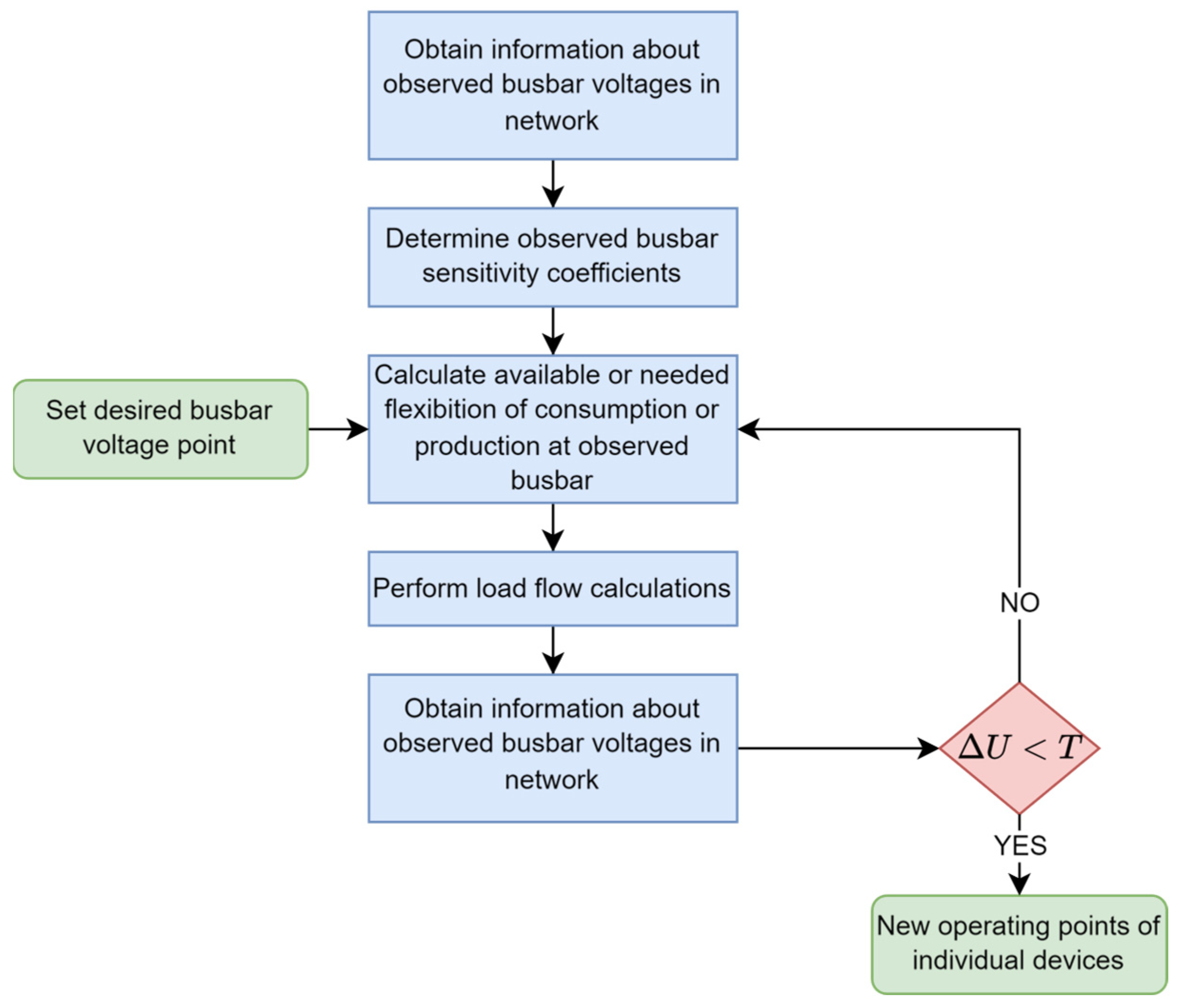
2.1. Problem Formulation and Improved Usage of Sensitivity Theory in LV Networks

Relationships between the nodal voltages and the nodal power injections are mathematically represented by the following matrix expression [16]:

$$\left[\begin{array}{c}\left[∆V\right]\\ \left[∆\vartheta \right]\end{array}\right]={\left[\begin{array}{cc}\left[\frac{\partial P}{\partial V}\right]& \left[\frac{\partial P}{\partial \vartheta }\right]\\ \left[\frac{\partial Q}{\partial V}\right]& \left[\frac{\partial Q}{\partial \vartheta }\right]\end{array}\right]}^{-1}\left[\begin{array}{cc}\left[1\right]& \left[0\right]\\ \left[0\right]& \left[1\right]\end{array}\right]\left[\begin{array}{c}\left[∆P^{*}\right]\\ \left[∆Q^{*}\right]\end{array}\right],$$

(1)

$$\left[S\right]={\left[\begin{array}{cc}\left[\frac{\partial P}{\partial V}\right]& \left[\frac{\partial P}{\partial \vartheta }\right]\\ \left[\frac{\partial Q}{\partial V}\right]& \left[\frac{\partial Q}{\partial \vartheta }\right]\end{array}\right]}^{-1}\left[\begin{array}{cc}\left[1\right]& \left[0\right]\\ \left[0\right]& \left[1\right]\end{array}\right],$$

(2)

where $\left[∆V\right]$ and $\left[∆\vartheta \right]$ represents the nodal voltage magnitudes and phase variations corresponding to the nodal active or reactive injections $\left[∆P^{*}\right]$ and $\left[∆Q^{*}\right]$. Equation (2) represents the sensitivity matrix.

Equations (1) and (2) can then be rewritten in a compact form:

$$\left[\begin{array}{c}\left[∆V\right]\\ \left[∆\vartheta \right]\end{array}\right]=\left[S\right]\left[\begin{array}{c}\left[∆P^{*}\right]\\ \left[∆Q^{*}\right]\end{array}\right].$$

(3)

Equation (3) can be simplified considering the fact that in radial networks only the voltage magnitude is needed to control the nodal voltages [16]. Consequently, the part with the phase angle can be omitted.

Differences between magnitudes of nodal voltages and the voltage $E_0$ in a radial network can be described with Equation (4):

$$V_{0i}=E_0-E_i,$$

(4)

where $E_0$ is the phase voltage at the LV busbar of the MV/LV transformer (where $E_0=V_n/\sqrt{3}$), and $E_i$ represents the phase voltage at $i$-th node. In radial networks, the voltage drop is equal to the sum of voltage differences across all connected nodes between the LV busbar and the i-th node, which can be mathematically described with Equation (5).

$$V_{0i}=\sum U_{ab},$$

(5)

where $U_{ab}$ is the voltage drop between adjacent nodes in the radial network between the LV busbar of the MV/LV transformer and the selected node i. The voltage magnitude at any node is therefore a function of the active and reactive components of currents:

$$U_{ab}=R_{ab}·I_{ab}·\mathit{cos}{\phi }_{ab}+X_{ab}·I_{ab}·\mathit{sin}{\phi }_{ab},$$

(6)

where $R_{ab}$ and $X_{ab}$ are the resistance and reactance of the line connecting nodes a and b, $I_{ab}$ is the current of that line, and $cos{\phi }_{ab}$ is the power factor. Equation (6) can now be multiplied by $\frac{U_b}{U_b}$, where $U_b$ is the voltage at node b:

$$U_{ab}=\frac{R_{ab}·I_{ab}·\mathit{cos}{\phi }_{ab}\cdot U_b+X_{ab}·I_{ab}·\mathit{sin}{\phi }_{ab}\cdot U_b}{U_b}=\frac{R_{ab}·P_b+X_{ab}·Q_b}{U_b}.$$

(7)

$P_b$ and $Q_b$ are now the sum of the active and reactive power of node b and all downstream nodes with respect to node b. Brenna et al. assume that nodal voltages are typically close to the nominal voltage of the network [16]. Equation (7) can then be simplified by replacing the voltage $U_b$ with the nominal voltage $E_N$:

$$U_{\mathrm{a}\mathrm{b}}=\frac{R_{ab}·P_b+X_{\mathrm{a}\mathrm{b}}·Q_b}{U_{\mathrm{b}}}\cong \frac{R_{\mathrm{a}\mathrm{b}}·P_b+X_{\mathrm{a}\mathrm{b}}·Q_b}{E_{\mathrm{N}}}.$$

(8)

However, this assumption is not necessarily true for LV radial distribution networks, as the need for flexibility arises when the maximum or minimum voltage in the network is 10% higher or lower than the voltage at the LV busbar of the MV/LV transformer. Additionally, the impedance of the MV/LV transformer in the LV network can not be neglected. An improvement of this method and its usage is described in the following subsection.

By utilizing Equations (5) and (8), it can be inferred that the voltage drops between the LV busbar of the MV/LV transformer and the selected node i depends on the sum of active and reactive powers of all the loads and generators connected to node i in the network topology. Additionally, Equations (9) and (10) define the total active and reactive power impacting the network at node i:

$${\mathsf{\Delta }P}_{\mathrm{i}}=P_{\mathrm{i}}^{in}-P_{\mathrm{i}}^{out},$$

(9)

$${\mathsf{\Delta }\mathrm{Q}}_{\mathrm{i}}=Q_{\mathrm{i}}^{in}-Q_{\mathrm{i}}^{out},$$

(10)

where the index above the variable indicates the power flowing into node i (in) and the power flowing out of node i (out). Now, the equation (5) can be reformulated and expressed as:

$$∆V_{\mathrm{i}}={\sum }_{j=1}^n\frac{\partial V_{\mathrm{i}}}{\partial P_{\mathrm{j}}}·∆P_{\mathrm{j}}+{\sum }_{j=1}^n\frac{\partial V_{\mathrm{i}}}{\partial Q_{\mathrm{j}}}·∆Q_{\mathrm{j}},$$

(11)

where the terms $\frac{\partial V_{\mathrm{i}}}{\partial P_{\mathrm{j}}}$ and $\frac{\partial V_{\mathrm{i}}}{\partial Q_{\mathrm{j}} }$ represent the difference in voltage that will occur at node i due to variations in the active and reactive power at node j. The entire system can be described in matrix form with Equations (12) and (13):

$$\left[S_{\mathrm{P}}\right]=\left[\begin{array}{cccc}\frac{\partial V_1}{\partial P_1}& \frac{\partial V_1}{\partial P_2}& \cdots & \frac{\partial V_1}{\partial P_{\mathrm{n}}}\\ \frac{\partial V_2}{\partial P_1}& \cdots & \cdots & \cdots \\ \cdots & \cdots & \cdots & \cdots \\ \frac{\partial V_{\mathrm{n}}}{\partial P_1}& \cdots & \cdots & \frac{\partial V_{\mathrm{n}}}{\partial P_{\mathrm{n}}}\end{array}\right],$$

(12)

$$\left[S_{\mathrm{Q}}\right]=\left[\begin{array}{cccc}\frac{\partial V_1}{\partial Q_1}& \frac{\partial V_1}{\partial Q_2}& \cdots & \frac{\partial V_1}{\partial Q_{\mathrm{n}}}\\ \frac{\partial V_2}{\partial Q_1}& \cdots & \cdots & \cdots \\ \cdots & \cdots & \cdots & \cdots \\ \frac{\partial V_{\mathrm{n}}}{\partial Q_1}& \cdots & \cdots & \frac{\partial V_{\mathrm{n}}}{\partial Q_{\mathrm{n}}}\end{array}\right].$$

(13)

Meanwhile, the individual elements of the sensitivity matrix can be expressed as:

$${\left(S_{\mathrm{P}}\right)}_{\mathrm{i}\mathrm{j}}=\frac{\partial V_{\mathrm{i}}}{\partial P_{\mathrm{j}}}=-\frac{R_{\mathrm{i}\mathrm{j}}}{E_{\mathrm{N}}},$$

(14)

$${\left(S_{\mathrm{Q}}\right)}_{\mathrm{i}\mathrm{j}}=\frac{\partial V_{\mathrm{i}}}{\partial Q_{\mathrm{j}}}=-\frac{X_{\mathrm{i}\mathrm{j}}}{E_{\mathrm{N}}},$$

(15)

where $R_{\mathrm{i}\mathrm{j}}$ and $X_{\mathrm{i}\mathrm{j}}$ are the sum of resistances and reactances of the lines according to the network topology.

In the previous literature, the authors did not consider the effect of the MV/LV transformer. The MV/LV transformer impedance should be considered, which means the final form of the individual elements of the sensitivity matrix is:

$${\left(S_{\mathrm{P}}\right)}_{\mathrm{i}\mathrm{j}}=\frac{\partial V_{\mathrm{i}}}{\partial P_{\mathrm{j}}}=-\left(\frac{R_{\mathrm{i}\mathrm{j}}}{E_{\mathrm{N}}}+Re\left(Z_{\mathrm{T}\mathrm{R}}\right)\right),$$

(16)

$${\left(S_{\mathrm{Q}}\right)}_{\mathrm{i}\mathrm{j}}=\frac{\partial V_{\mathrm{i}}}{\partial Q_{\mathrm{j}}}=-\left(\frac{X_{\mathrm{i}\mathrm{j}}}{E_{\mathrm{N}}}+Im\left(Z_{\mathrm{T}\mathrm{R}}\right)\right).$$

(17)

As described before, the term $U_{\mathrm{b}}$ in Equation (8) is replaced with the term $E_{\mathrm{N}}$, introducing an error in calculation results when the voltage difference in the network arises. Based on experience from the distribution system operators (DSOs) the maximum or minimum voltage in the network can deviate for more than 10% from $E_{\mathrm{N}}$. To minimize the computational error, we propose an implementation of a while loop until the desired tolerance of results is achieved. The proposed flow chart is presented in Figure 1.

Sensitivity Theory Use Case Example

For a better understanding, a simple example of a matrix system of sensitivity coefficients is presented below for a simple LV radial network, depicted in Figure 2. P and Q represent active and reactive power injections in a given node indicated with the letter N. R and X embody line resistance and reactance, respectively. MV/LV TR is a transformer, which transforms voltage from MV level to LV level.

Firstly, the voltage deviation caused by individual elements in the network is represented in matrix form as:

$$\left[\begin{array}{c}∆V_1\\ ∆V_2\\ ∆V_3\\ ∆V_4\end{array}\right]=\left[\begin{array}{cccc}\frac{\partial V_1}{\partial P_1}& \frac{\partial V_1}{\partial P_2}& \frac{\partial V_1}{\partial P_3}& \frac{\partial V_1}{\partial P_4}\\ \frac{\partial V_2}{\partial P_1}& \frac{\partial V_2}{\partial P_2}& \frac{\partial V_2}{\partial P_3}& \frac{\partial V_2}{\partial P_4}\\ \frac{\partial V_3}{\partial P_1}& \frac{\partial V_3}{\partial P_2}& \frac{\partial V_3}{\partial P_3}& \frac{\partial V_3}{\partial P_4}\\ \frac{\partial V_4}{\partial P_1}& \frac{\partial V_4}{\partial P_2}& \frac{\partial V_4}{\partial P_3}& \frac{\partial V_4}{\partial P_4}\end{array}\right]\left[\begin{array}{c}∆P_1\\ ∆P_2\\ ∆P_3\\ ∆P_4\end{array}\right]+\left[\begin{array}{cccc}\frac{\partial V_1}{\partial Q_1}& \frac{\partial V_1}{\partial Q_2}& \frac{\partial V_1}{\partial Q_3}& \frac{\partial V_1}{\partial Q_4}\\ \frac{\partial V_2}{\partial Q_1}& \frac{\partial V_2}{\partial Q_2}& \frac{\partial V_2}{\partial Q_3}& \frac{\partial V_2}{\partial Q_4}\\ \frac{\partial V_3}{\partial Q_1}& \frac{\partial V_3}{\partial Q_2}& \frac{\partial V_3}{\partial Q_3}& \frac{\partial V_3}{\partial Q_4}\\ \frac{\partial V_4}{\partial Q_1}& \frac{\partial V_4}{\partial Q_2}& \frac{\partial V_4}{\partial Q_3}& \frac{\partial V_4}{\partial Q_4}\end{array}\right]\left[\begin{array}{c}∆Q_1\\ ∆Q_2\\ ∆Q_3\\ ∆Q_4\end{array}\right].$$

(18)

By considering expressions (14) and (15), the matrix of sensitivity coefficients for the active and reactive components can be rewritten as:

$$\left[S_{\mathrm{P}}\right]=-\frac{1}{E_{\mathrm{N}}}\left(\left[\begin{array}{cccc}{R}_1& R_1& R_1& R_1\\ R_1& R_1+R_2& R_1+R_2& R_1+R_2\\ R_1& R_1+R_2& R_1+R_2+R_3& R_1+R_2\\ R_1& R_1+R_2& R_1+R_2& R_1+R_2+R_4\end{array}\right]+Re(Z_{\mathrm{T}\mathrm{R}})\right),$$

(19)

$$\left[S_{\mathrm{Q}}\right]=-\frac{1}{E_{\mathrm{N}}}\left(\left[\begin{array}{cccc}{X}_1& X_1& X_1& X_1\\ X_1& X_1+X_2& X_1+X_2& X_1+X_2\\ X_1& X_1+X_2& X_1+X_2+X_3& X_1+X_2\\ X_1& X_1+X_2& X_1+X_2& X_1+X_2+X_4\end{array}\right]+Im\left(Z_{\mathrm{T}\mathrm{R}}\right)\right).$$

(20)

The sensitivity coefficients obtained from expressions (19) and (20) indicate which loads have a greater impact on the voltage change at a specific node (for the same power change). For the first node, all sensitivity coefficients have equal values, meaning that the power change of any load will have an equal impact on the voltage at node 1. For the second node, it is evident that the loads at nodes 2, 3, and 4 have a greater influence on the voltage change at node 2 compared to node 1. The voltage at node 3 will be most affected by the power change of the load at that node, which is mathematically represented with expression (21). The same applies to node 4, where the voltage will be most affected by the change in load power at node 4.

$$\begin{gathered} \frac{\partial V_3}{\partial P_1}=-\frac{R_1}{E_{\mathrm{N}}} \\ \frac{\partial V_3}{\partial P_2}=-\frac{R_1+R_2}{E_{\mathrm{N}}} \\ \frac{\partial V_3}{\partial P_3}=-\frac{R_1+R_2+R_3}{E_{\mathrm{N}}} \\ \frac{\partial V_3}{\partial P_4}=-\frac{R_1+R_2}{E_{\mathrm{N}}} \end{gathered}$$

(21)

From expression (22) it is also evident that the change in load power at node 2 has an equal influence on the voltage at nodes 3 and 4.

$$\begin{gathered} \frac{\partial V_3}{\partial P_2}=-\frac{R_1+R_2}{E_{\mathrm{N}}} \\ \frac{\partial V_4}{\partial P_2}=-\frac{R_1+R_2}{E_{\mathrm{N}}} \end{gathered}$$

(22)

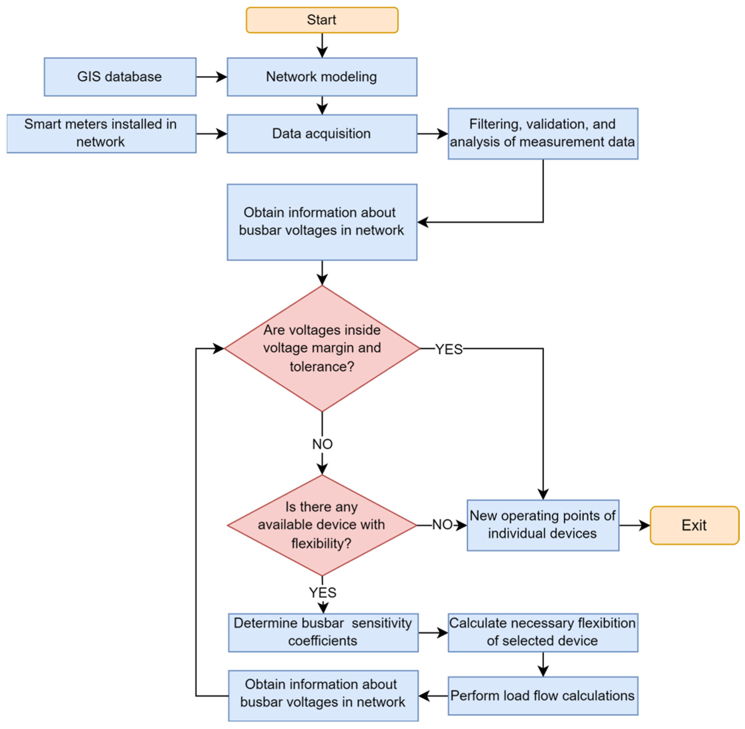
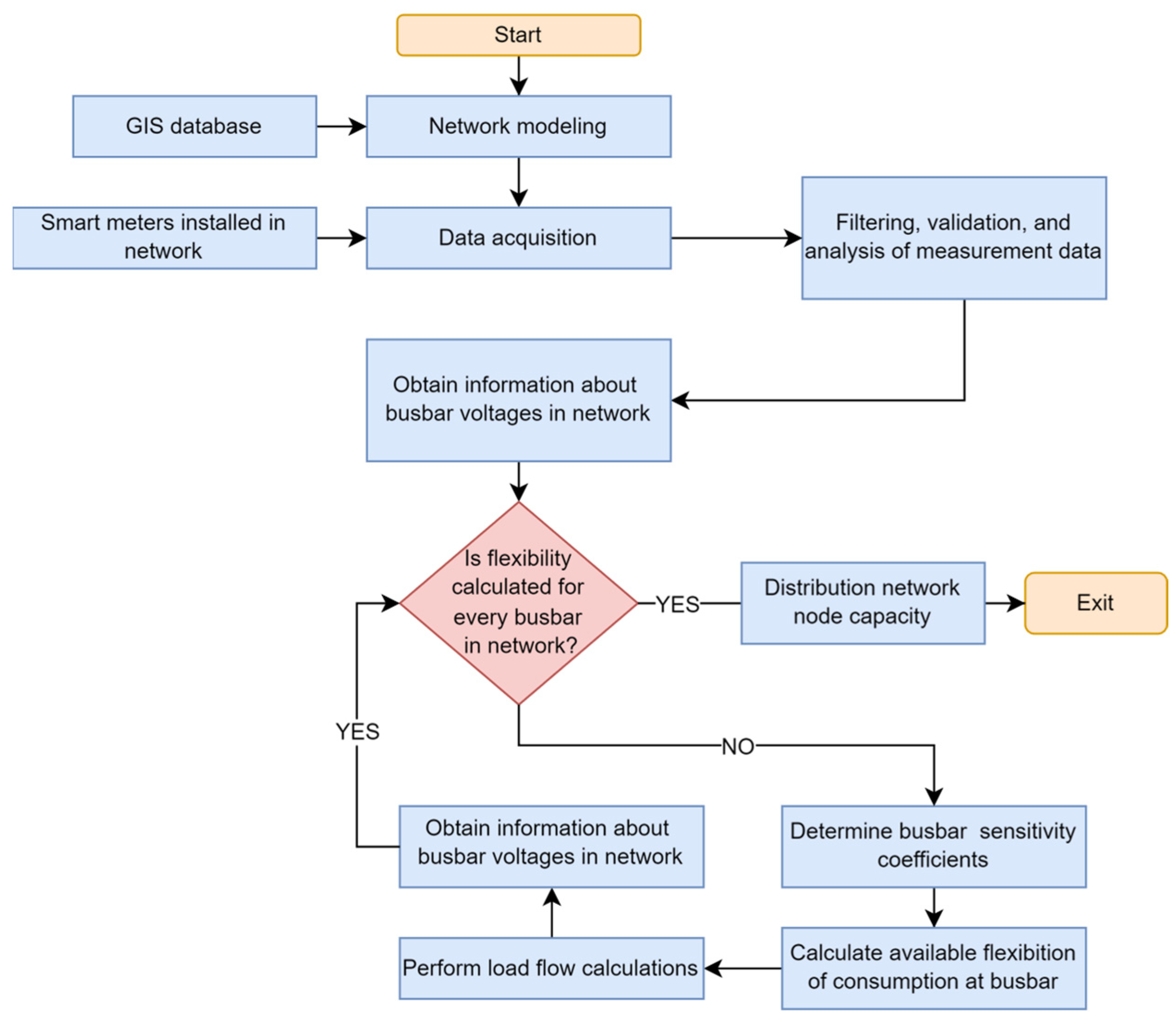
3. Flexibility and Distribution Network’s Operating Criteria

Flexibility can be primarily utilized in the operation of LV networks when the network operates outside of the set or standard required operating conditions, such as minimal voltage, maximal voltage, or transformer loading. The consideration of flexibility in the planning phase is described in [6]. When flexibility is applied in the operation phase we follow the process described in Figure 3. The first three steps are always the same. Then, based on the network conditions, one of the two proposed subprocesses is executed. The subprocesses are described in more detail below.

When the conditions in the network are not within operational criteria, Subprocess 1 is executed. The detailed flowchart of Subprocess 1 is presented in Figure 4. Based on measurement analysis, the busbar with the largest voltage deviation is identified. Then, the row of sensitivity coefficients corresponding to that busbar is extracted from the sensitivity coefficient matrix. Considering the information about devices (users) that can provide flexibility, the coefficients are sorted from the highest to the lowest. This way, the maximum impact on voltage with the minimum power change will be achieved. Once the necessary power change is determined, based on the coefficient, load flow calculations are performed using the pandapower library [26]. This provides the algorithm with information about the busbars voltages after the flexibility is provided. As described in the previous subsection, due to the complexity of the calculation, the term $U_b$ in Equation (7) is replaced with the term $E_N$, introducing a computational error that is resolved by iterative calculation until the desired tolerance of results is achieved. If a single device cannot provide sufficient flexibility, the device with the second-highest coefficient is selected, etc. Additionally, the information about the activation of individual devices is stored, thereby updating the availability of devices in near real-time. The result of the algorithm is the new operating points of individual devices.

In a case when the distribution network operates within operating criteria, devices can utilize their flexibility to provide system services for other power system stakeholders. Subprocess 2 which is presented in Figure 5, is similar to the one described before. The main difference is that in this case, the distribution network node capacity, i.e., maximal nodal powers that still allow network operation within operational limits, is determined. The algorithm selects the highest coefficient value for each busbar. Once the allowable power change in consumption, based on the coefficient, is determined, load flow calculations are performed using the pandapower library, which, as described in the previous subsection, eliminates computational errors that arise from the use of the simplified sensitivity coefficient matrix.

4. Application Example

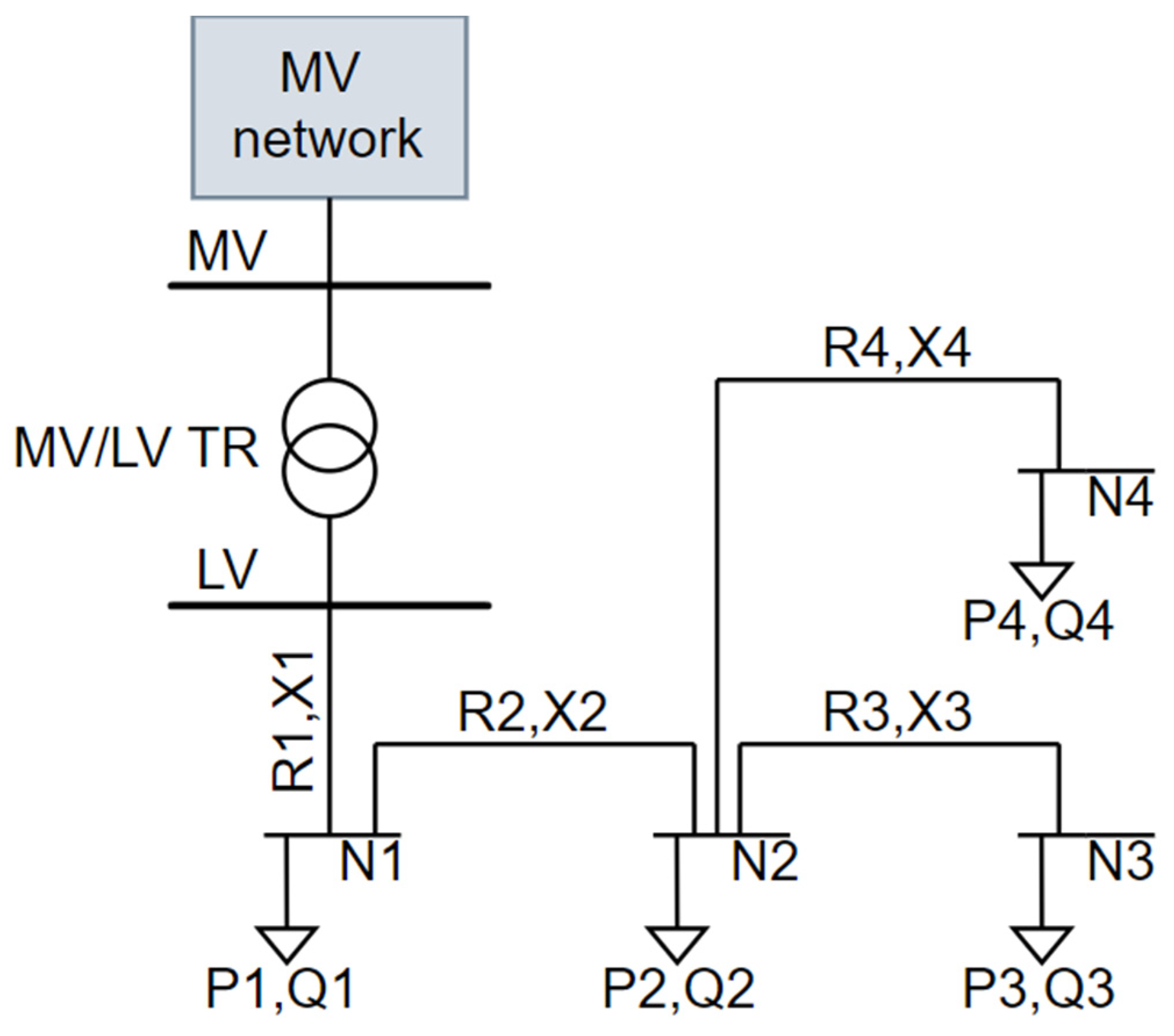
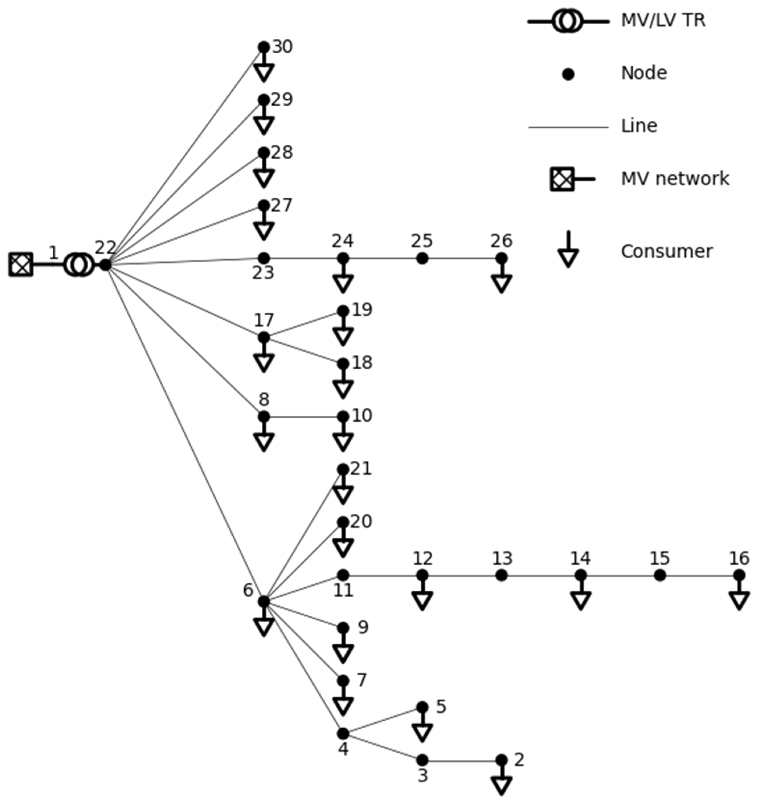
To illustrate the practical implementation of the proposed method and to evaluate its efficiency, the analysis is demonstrated on a real LV distribution network model, which is also used as a pilot site to test the proposed method in an actual operating LV distribution network. A simplified scheme of the analyzed system is shown in Figure 6.

4.1. Network Data

As can be observed from Figure 6, there is one 20/0.4 kV transformer (MV/LV TR), which is supplying the LV network and is not overloaded in the current state. There are six photovoltaics (PVs) installed in the network (two at node 19), which can provide flexibility in case of overvoltages. For demonstrational purposes, three additional battery storage systems were deployed at three PV sites. One battery storage system has a capacity of 12 kWh and a peak power of 5 kW. A total of 26 consumers are connected to the network (two consumers are connected to busses 2, 9, 12, 20, and 28). The network consists of 28 lines, which are described in detail in Appendix A in

Table A1. Low-voltage distribution network parameters.

Component	Parameter	Value	Component	Parameter	Value
MV/LV TR	S $u_k$ $P_{\mathrm{F}\mathrm{e}}$ $U_n$	100 kVA 4% 1.73 kW 20/0.4 kV	Line 15 @22-17	R X l	0.443 ohm/km 0.080 ohm/km 0.234 km
Line 1 @3-2	R X l	0.442 ohm/km 0.079 ohm/km 0.223 km	Line 16 @17-18	R X l	0.868 ohm/km 0.083 ohm/km 0.025 km
Line 2 @4-3	R X l	0.442 ohm/km 0.079 ohm/km 0.055 km	Line 17 @17-19	R X l	0.868 ohm/km 0.083 ohm/km 0.028 km
Line 3 @4-5	R X l	0.442 ohm/km 0.079 ohm/km 0.228 km	Line 18 @6-20	R X l	0.443 ohm/km 0.082 ohm/km 0.037 km
Line 4 @6-4	R X l	0.125 ohm/km 0.079 ohm/km 0.0.149 km	Line 19 @6-21	R X l	0.443 ohm/km 0.082 ohm/km 0.046 km
Line 5 @6-7	R X l	0.443 ohm/km 0.082 ohm/km 0.069 km	Line 20 @22-6	R X l	0.125 ohm/km 0.079 ohm/km 0.098 km
Line 6 @22-29	R X l	0.442 ohm/km 0.079 ohm/km 0.005 km	Line 21 @22-23	R X l	0.442 ohm/km 0.079 ohm/km 0.043 km
Line 7 @6-9	R X l	0.443 ohm/km 0.082 ohm/km 0.176 km	Line 22 @23-24	R X l	0.442 ohm/km 0.079 ohm/km 0.004 km
Line 8 @8-10	R X l	3.03 ohm/km 0.1 ohm/km 0.032 km	Line 23 @24-25	R X l	0.442 ohm/km 0.079 ohm/km 0.004 km
Line 9 @6-11	R X l	0.443 ohm/km 0.082 ohm/km 0.057 km	Line 24 @25-26	R X l	0.868 ohm/km 0.083 ohm/km 0.026 km
Line 10 @11-12	R X l	0.641 ohm/km 0.080 ohm/km 0.059 km	Line 25 @22-27	R X l	0.443 ohm/km 0.082 ohm/km 0.047 km
Line 11 @12-13	R X l	0.641 ohm/km 0.083 ohm/km 0.042 km	Line 26 @22-28	R X l	0.442 ohm/km 0.079 ohm/km 0.018 km
Line 12 @13-14	R X l	0.442 ohm/km 0.079 ohm/km 0.032 km	Line 27 @22-30	R X l	0.442 ohm/km 0.079 ohm/km 0.035 km
Line 13 @14-15	R X l	0.442 ohm/km 0.079 ohm/km 0.031 km	Line 28 @22-8	R X l	0.868 ohm/km 0.083 ohm/km 0.049 km
Line 14 @15-16	R X l	0.442 ohm/km 0.079 ohm/km 0.018 km

among other network parameters.

4.2. Simulation Results

The analysis of the voltage regulation was performed according to the algorithm, presented in Section 3. Two scenarios were simulated. In the first scenario, only the six PVs provide needed flexibility, by setting their active power setpoints based on sensitivity matrix coefficients. The second scenario represents the possibility of using flexibility when DN is working inside operational criteria. Distribution network node capacities are calculated using the sensitivity theory. The operating criteria in all three scenarios are specified so that all nodal voltages remain within the range of [1.0–1.035] p.u., while the current must not exceed the thermal limits of network elements. The selected range of nodal voltages is for the sake of a more adequate representation of the usage of the method. The voltage set point of the external grid, which represents the MV part of the network, is set to 1.03 p.u.

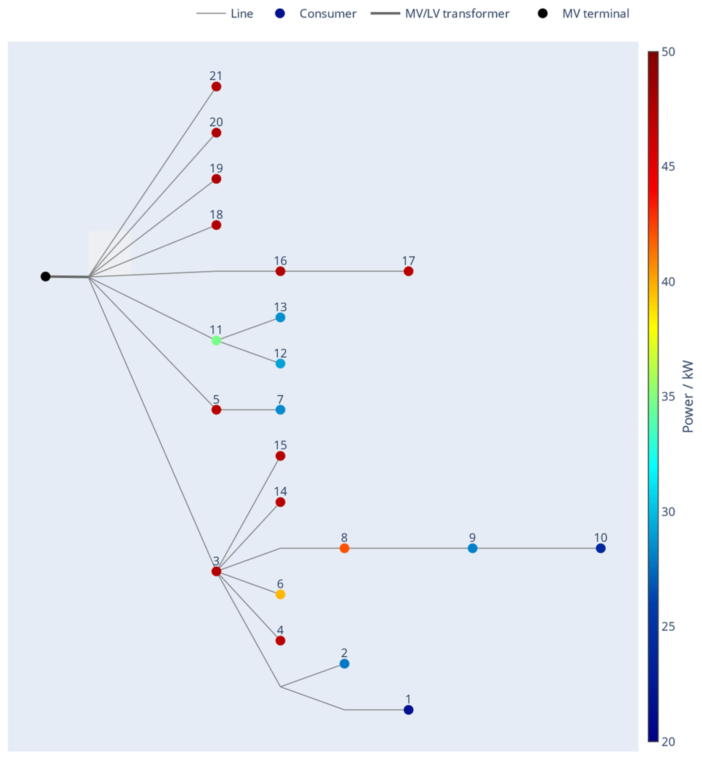
4.2.1. First Scenario

In the first scenario, the sensitivity coefficient method is used to define new working points for individual solar power plants. The objective was to maximize the cumulative active power generation of all PVs while considering the existing network infrastructure limits. In other words, this sum represents the network’s hosting capacity. Additionally, the viability of the method was defined by two metrics:

• Whether the network operated within operating criteria after determining the new active power set points of individual PV.
• The required computational time of the method.

Table 1. Individual active power set points of PVs and the sum of active power of PVs in kW in scenario 1.

	${\mathit{P}}_{\mathbf{P}\mathbf{V},19}$	${\mathit{P}}_{\mathbf{P}\mathbf{V},19}$	${\mathit{P}}_{\mathbf{P}\mathbf{V},23}$	${\mathit{P}}_{\mathbf{P}\mathbf{V},25}$	${\mathit{P}}_{\mathbf{P}\mathbf{V},18}$	${\mathit{P}}_{\mathbf{P}\mathbf{V},16}$	$\mathsf{\Sigma }\mathit{P}$
Initial state	20.0	20.0	20.0	20.0	20.0	20.0	120.0
Method with sens. coef.	19.0	20.0	20.0	9.4	0.0	12.8	8.2

and

Table 2. Simulation results in scenario 1.

	${\mathit{S}}_{\mathbf{T}\mathbf{R}}$/p.u.	${\mathit{V}}_{\mathbf{m}\mathbf{i}\mathbf{n}}$/p.u.	${\mathit{V}}_{\mathbf{m}\mathbf{a}\mathbf{x}}$/p.u.	${\mathit{I}}_{\mathbf{l},\mathbf{m}\mathbf{a}\mathbf{x}}$/p.u.	$\mathit{t}/\mathbf{s}$
Initial state	0.65	1.028	1.055	0.29	/
Method with sens. coef.	0.28	1.027	1.035	0.28	1

present the results of the initial state of the network and the state of the network after setting the new active power set points of the PVs. In scenario 1, the active power set point of all consumers was set to 2 kW, while their reactive power was set to 0 kVAr. The initial active power set point of all solar power plants was set to 20 kW. Table 1 displays individual active power set points of PVs and the sum of all these set points, while Table 2 presents the simulation results, combining data on transformer power, minimum and maximum voltages in the network, and the highest value of line current amplitudes. The index of PV in Table 1 indicates the node where the PV system is installed. For the sensitivity coefficient method, Table 2 also includes the time it took for the method to return the results.

According to the results given in Table 2, it can be observed that the operating criteria were violated in the initial state of the network, as the maximum voltage in the network reached 1.055 p.u. This means that some actions need to be performed in the network, which involved reducing the active power output of the solar power plants, where we obtained new setpoints for PVs using the sensitivity coefficients-based method.

Based on the results in Table 2, we can assert that the method was successful since the maximum voltage is now 1.035 p.u., which means that we are at the upper limit of the operating criteria. At the same time, this point represents the network’s hosting capacity at the given moment. This implies that the presented configuration of active power set points for PVs obtained with this method will ensure the maximum power generation of the solar power plants while adhering to the set operating criteria. The time complexity of the presented method is very low, as indicated in the last column of Table 2. This means that this method can be applied in applications that operate near real-time.

Figure 7 shows the voltage conditions throughout the entire network in the initial state and at the state after the PVs active power curtailment. From Figure 7 we can see that the highest voltages occur at terminals 17, 18, and 19, where there is a significant injection of power generated by PVs electrically far from the transformer. Without the executed maneuver, the distribution operator would have to conventionally reinforce the network to address these issues. Figure 7 also visually illustrates the normalization of conditions in the network, which operates within the set operating criteria after the maneuver.

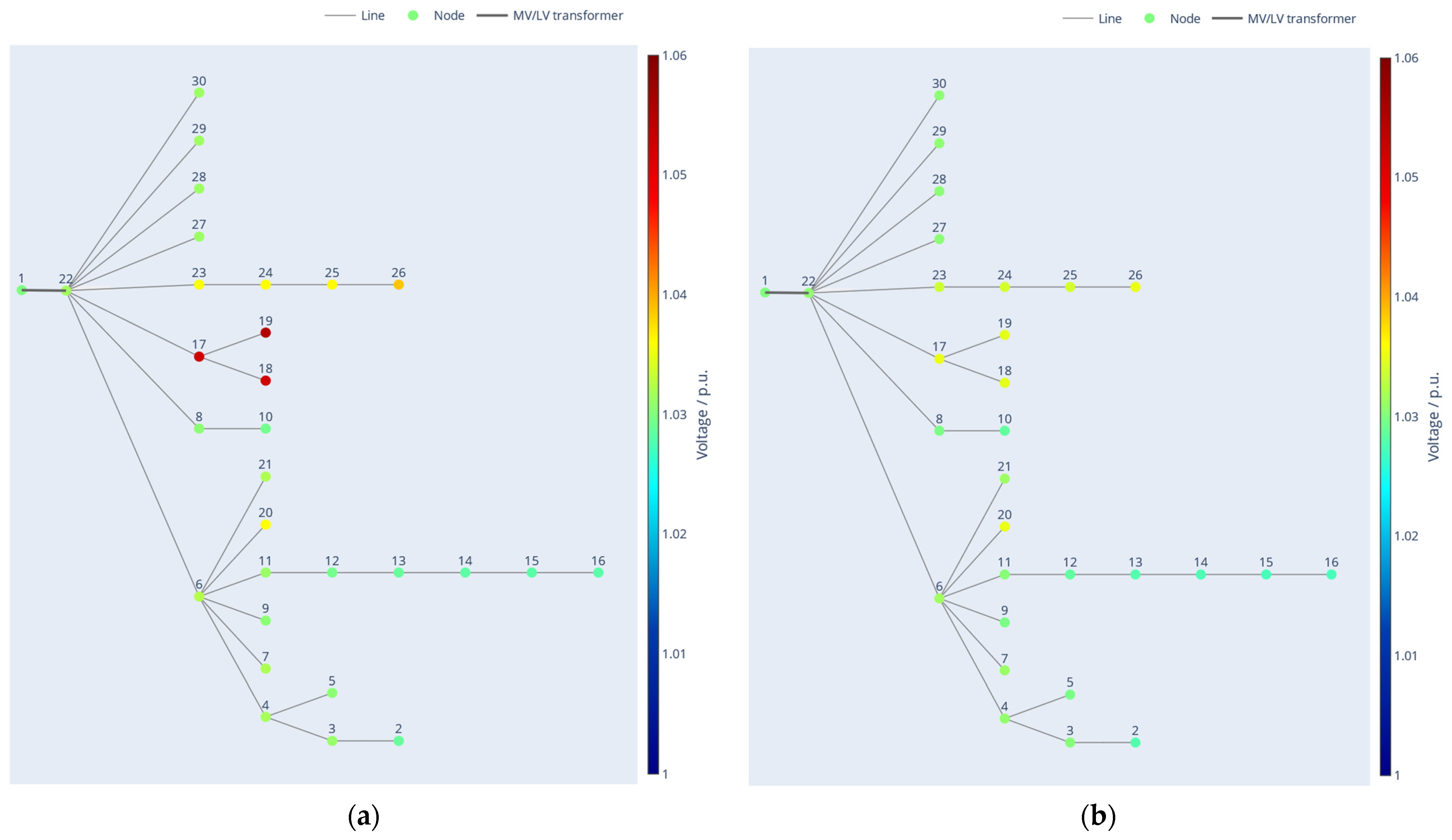
4.2.2. Second Scenario

As mentioned in Section 2, providing flexibility when the power distribution network operates within operational criteria could represent a potential for implementing system services such as tertiary or secondary frequency control (aFRR and mFRR services). For this purpose, the node capacity of the power distribution network is calculated. Calculations are once again computed using the sensitivity coefficients method. This method is suitable for applications operating in near real-time. The analyzed network and operational criteria remain the same as in Section 4.2.1. The active power at all consumption points was initially set to 2 kW, while reactive power was set to 0 kVAr.

The results are visualized in the form of a heat map in Figure 8. Since we can only change the active power at the consumption points of the low-voltage network, only their nodal capacities are shown. The analysis revealed that the consumer 1 in Figure 8 has the smallest nodal connection capacity. Here, the limiting factor was the minimum allowed voltage value. It is clearly visible from the map that nodes electrically close to the transformer have the same node capacity. The rated power of the transformer was set as the limiting factor. In absolute terms, this means that in the analyzed scenario, the lowest node connection capacity is 22 kW, while the highest value is 48 kW. Due to the algorithm’s speed, node connection capacities could be updated in a very short time interval, enabling the aggregator to provide system services, and ensuring that the power distribution network operates within operational criteria.

5. Conclusions

The main objective of this paper is to propose the design of the algorithm for managing the flexibility of consumption and production in distribution networks based on the sensitivity coefficients method. Modern low-voltage distribution networks are facing significant challenges due to the introduction of previously unknown types of loads, such as electric vehicles or heat pumps, and the increasing share of renewable energy sources, especially solar energy. To ensure that networks will operate within desired operational criteria in the future, information about the hosting capacity of individual networks and nodes is necessary. The concept of hosting capacity, considering the operational limitations of the distribution network, has been used in the field of electrical engineering for some time. However, in most cases, it is used only for the planning of distribution networks. The sensitivity coefficients method has been recognized as a potential method for designing an algorithm for managing the flexibility of consumption and production within power distribution network operations.

The functionality of such an algorithm was simulated on a real low-voltage distribution network model. To model the network and calculate power flows, an open-source library pandapower was used, implemented in the Python 3.10 programming language. Data from the real network model received in the form of a GIS database, were organized and connected to the mathematical model of the network. Then the sensitivity coefficients method was implemented in the Python programming language.

The case study presents only the PV generation management because in the demo site aggregator can only control the generation of PV systems and battery energy systems so that the bus voltages do not exceed the set maximum limits. The initial algorithm was then upgraded to be able to control also the load demand and to be used for determining DNNC as described in Section 3.

In the first scenario of the algorithm test, the network operation state was set outside of the operational limits. The success of the method was determined by two criteria. The first criterion was whether the network operated within the operational criteria after setting new operating points for individual PVs. The second criterion represented the time needed to calculate the new operating points for PVs. The simulation results show that sensitivity-based methods, by setting new operating points, ensured that the network operates within the set operational criteria. The sensitivity coefficients method obtained these points in a very short time, which is a crucial feature for implementation in applications operating in near real-time.

The second part of the test represented a scenario where the network operates within the set operational criteria. In this part, the goal was to determine the maximum power change at each node while still maintaining the network within the operational limits. The sensitivity coefficients method was used for this purpose, and the result was a map showing the parts of the network where a higher power change is possible.

This model is already being implemented and in the testing phase on the virtual machine inside DSO Elektro Gorenjska IT architecture. The model is sampling voltage, current, and power injections with a 1-min resolution. An operator can set the desired network maximum voltage setpoint. Based on that setpoint, needed flexibility is calculated and sent in a standardized XML format to the aggregator who activates battery storage or sets active power setpoint of PVs. The standard format also enables the usage of flexibility on the demand side. Due to the low calculation time, computations using the proposed algorithm can handle the 1-min sampling rate. Standardized XML format enables usage of this model also after the end of the demo project. Our model is not load type sensitive since DSO can also manually set the maximum active power change in one node based on its evidence or experience. This approach enables DSO can combine flexibility from different aggregators and different load types since the model returns needed flexibility per node and not per device. That also means that aggregators are responsible for all load operations.

This algorithm will serve as a basis for implementing flexibility services within a demo project in a Slovenian LV distribution network. The overall objective of this project is the creation of a local flexibility market platform, which will enable the exploitation of the network customer’s flexibility for distribution network operation and for the provision of services to other power system stakeholders. This approach will result in an increase in the network hosting capacity and asset utilization, reducing substantially the costs for network reinforcement.

References

1. Knez, K. Zasnova Algoritma za Vodenje Prožnosti Odjema in Proizvodnje v Distribucijskih Omrežjih. Master’s Thesis, Univerza v Ljubljani, Fakulteta za Elektrotehniko, Ljubljana, Slovenia, 2023. Available online: https://repozitorij.uni-lj.si/IzpisGradiva.php?id=147015 (accessed on 28 June 2023).
2. You, S.; Bindner, H.W.; Hu, J.; Douglass, P.J. An overview of trends in distribution network planning: A movement towards smart planning. In Proceedings of the 2014 IEEE PES T&D Conference and Exposition, Chicago, IL, USA, 14–17 April 2014; pp. 1–5. [Google Scholar] [CrossRef]
3. Iweh, C.D.; Gyamfi, S.; Tanyi, E.; Effah-Donyina, E. Distributed Generation and Renewable Energy Integration into the Grid: Prerequisites, Push Factors, Practical Options, Issues and Merits. Energies 2021, 14, 5375. [Google Scholar] [CrossRef]
4. Shafiullah, G. Impacts of renewable energy integration into the high voltage (HV) networks. In Proceedings of the 2016 4th International Conference on the Development in the in Renewable Energy Technology (ICDRET), Dhaka, Bangladesh, 7–9 January 2016; pp. 1–7. [Google Scholar] [CrossRef]
5. De Almeida Torres, T.J.P. Comparision between Traditional Network Reinforcement and the Use of DER Flexibility. October 2020. Available online: https://repositorio-aberto.up.pt/handle/10216/132859 (accessed on 4 July 2023).
6. Blažič, B.; Herman, L.; Ilkovski, M.; Knez, K. D3.1: Metodologija in Orodje za Načrtovanje Pametnih Omrežij; Fakulteta za elektrotehniko: Ljubljana, Slovenia, 2023. [Google Scholar]
7. Hashemi, S.; Østergaard, J. Methods and strategies for overvoltage prevention in low voltage distribution systems with PV. IET Renew. Power Gener. 2017, 11, 205–214. [Google Scholar] [CrossRef]
8. Zhou, Q.; Bialek, J.W. Generation curtailment to manage voltage constraints in distribution networks. IET Gener. Transm. Distrib. 2007, 1, 492–498. [Google Scholar] [CrossRef]
9. Mehinovic, A.; Zajc, M.; Suljanovic, N. Interpretation and Quantification of the Flexibility Sources Location on the Flexibility Service in the Distribution Grid. Energies 2023, 16, 590. [Google Scholar] [CrossRef]
10. Demirok, E.; Sera, D.; Teodorescu, R.; Rodriguez, P.; Borup, U. Evaluation of the voltage support strategies for the low voltage grid connected PV generators. In Proceedings of the 2010 IEEE Energy Conversion Congress and Exposition, Atlanta, GA, USA, 12–16 September 2010; pp. 710–717. [Google Scholar] [CrossRef]
11. Dib, M.; Ramzi, M.; Nejmi, A. Voltage regulation in the medium voltage distribution grid in the presence of renewable energy sources. Mater. Today Proc. 2019, 13, 739–745. [Google Scholar] [CrossRef]
12. Karimi, M.; Mokhlis, H.; Naidu, K.; Uddin, S.; Bakar, A.H.A. Photovoltaic penetration issues and impacts in distribution network—A review. Renew. Sustain. Energy Rev. 2016, 53, 594–605. [Google Scholar] [CrossRef]
13. Putrus, G.A.; Suwanapingkarl, P.; Johnston, D.; Bentley, E.C.; Narayana, M. Impact of electric vehicles on power distribution networks. In Proceedings of the 2009 IEEE Vehicle Power and Propulsion Conference, Dearborn, MI, USA, 7–10 September 2009; pp. 827–831. [Google Scholar] [CrossRef]
14. Honarmand, M.E.; Hosseinnezhad, V.; Hayes, B.; Siano, P. Local Energy Trading in Future Distribution Systems. Energies 2021, 14, 3110. [Google Scholar] [CrossRef]
15. Olivella-Rosell, P.; Lloret-Gallego, P.; Munné-Collado, Í.; Villafafila-Robles, R.; Sumper, A.; Ottessen, S.Ø.; Rajasekharan, J.; Bremdal, B.A. Local Flexibility Market Design for Aggregators Providing Multiple Flexibility Services at Distribution Network Level. Energies 2018, 11, 822. [Google Scholar] [CrossRef]
16. Brenna, M.; Berardinis, E.D.; Foiadelli, F.; Sapienza, G.; Zaninelli, D. Voltage Control in Smart Grids: An Approach Based on Sensitivity Theory. J. Electromagn. Anal. Appl. 2010, 2010, 2591. [Google Scholar] [CrossRef]
17. Bakhshideh Zad, B.; Hasanvand, H.; Lobry, J.; Vallée, F. Optimal reactive power control of DGs for voltage regulation of MV distribution systems using sensitivity analysis method and PSO algorithm. Int. J. Electr. Power Energy Syst. 2015, 68, 52–60. [Google Scholar] [CrossRef]
18. Džafić, I.; Jabr, R.A.; Halilovic, E.; Pal, B.C. A Sensitivity Approach to Model Local Voltage Controllers in Distribution Networks. IEEE Trans. Power Syst. 2014, 29, 1419–1428. [Google Scholar] [CrossRef]
19. Kim, Y.-J. Development and Analysis of a Sensitivity Matrix of a Three-Phase Voltage Unbalance Factor. IEEE Trans. Power Syst. 2018, 33, 3192–3195. [Google Scholar] [CrossRef]
20. Wang, S.; Liu, Q.; Ji, X. A Fast Sensitivity Method for Determining Line Loss and Node Voltages in Active Distribution Network. IEEE Trans. Power Syst. 2018, 33, 1148–1150. [Google Scholar] [CrossRef]
21. Zhu, X.; Wang, J.; Mulcahy, D.; Lubkeman, D.L.; Lu, N.; Samaan, N.; Huang, R. Voltage-load sensitivity matrix based demand response for voltage control in high solar penetration distribution feeders. In Proceedings of the 2017 IEEE Power & Energy Society General Meeting, Chicago, IL, USA, 16–20 July 2017; pp. 1–5. [Google Scholar] [CrossRef]
22. Di Fazio, A.R.; Russo, M.; Valeri, S.; De Santis, M. Sensitivity-Based Model of Low Voltage Distribution Systems with Distributed Energy Resources. Energies 2016, 9, 801. [Google Scholar] [CrossRef]
23. Zhang, L.; Zhao, C.; Zhang, B.; Li, G.; Tang, W. Voltage control method based on three-phase four-wire sensitivity for hybrid AC/DC low-voltage distribution networks with high-penetration PVs. IET Renew. Power Gener. 2022, 16, 700–712. [Google Scholar] [CrossRef]
24. Napredno Merjenje Porabe—Agencija za Energijo. Available online: https://www.agen-rs.si/gospodinjski/elektrika/napredno-merjenje-porabe (accessed on 23 November 2022).
25. Dovnik, I.; Buh, T.; Podbelšek, I. Zajem Merilnih Podatkov Iz Sistemskih Števcev El. Energije z Uporabo Naprednih Spletnih Storitev. In Proceedings of the 13. Konferenca Slovenskih Elektroenergetikov CIGRE-CIRED, Maribor, Denmark, 22–24 May 2017; p. 8. [Google Scholar]
26. Pandapower—Pandapower 2.12.1 Documentation. Available online: https://pandapower.readthedocs.io/en/latest/ (accessed on 27 April 2023).
Figure 1. Minimalization of the computational error.
Energies 17 01783 g001
Figure 2. Simplified LV radial network.
Energies 17 01783 g002
Figure 3. Proposed flowchart when the flexibility is used in the operation phase.
Energies 17 01783 g003
Figure 4. Algorithm flowchart when distribution network (DN) is operating outside operating criteria.
Energies 17 01783 g004
Figure 5. Algorithm flowchart when DN is operating inside operating criteria.
Energies 17 01783 g005
Figure 6. Single line diagram of the modeled low-voltage distribution network.
Energies 17 01783 g006
Figure 7. Grid simulation result visualization. (a) visualizes the voltage results obtained from simulation in the initial conditions. (b) visualizes the voltage results obtained from simulation after maneuver was performed.
Energies 17 01783 g007
Figure 8. Calculated node capacity result visualization when power distribution network is operating inside operating criteria.
Energies 17 01783 g008