Dynamic Patterns in the Small-Signal Behavior of Power Systems with Wind Power Generation

Abstract

This paper investigates the dynamic patterns in the small-signal behavior of power systems with wind power generation. The interactions between synchronous generators and wind generators are investigated. In addition, the impact of increased wind generation penetration on the damping and frequency of the synchronous generator’s electromechanical oscillations is addressed. Wind generators of three different technologies are considered throughout this study. Very detailed dynamic models of wind generators are used and detailed.

1. Introduction

The investigation of the small-signal behavior of power systems requires the use of appropriate models. The models of synchronous generators needed to study the rotor angle’s small-signal stability are well-established in the technical literature [1] and are called electromechanical models. Rotor angle small-signal stability is concerned with poorly damped oscillations of the frequency, voltage, and power in the frequency range between 0.1 and 2 Hz. Such oscillations are usually called electromechanical oscillations since they originate in the oscillation of the synchronous generator rotors.

Massively incorporating inverter-based generation into power systems has led to new forms of power system stability called resonance stability and converter-driven stability [2]. The investigation of such forms of stability requests much more detailed models (electromagnetic models) instead of the electromechanical models used to study rotor angle small-signal stability.

The study of the effect of wind power generation on the damping and frequency of power system electromechanical oscillations has been addressed using simplified models of wind generators (see [3,4,5,6,7,8]) in which the machine dynamics have been neglected and the dynamics of inner current controllers have been assumed to be ideal. Moreover, the design of damping controllers has been conducted using such simplified models [9,10].

This paper investigates the dynamic patterns in the small-signal behavior of power systems with wind generation. Dynamic patterns are close associations between state variables and eigenvalues of the linear model of a dynamic system. The aim of our study is to provide a foundation for the modeling practices of wind generation for the rotor-angle small-signal stability of power systems. Hence, the interaction between synchronous and wind generators is studied. In addition, the variation in the damping and frequency of the electromechanical oscillation of a synchronous generator connected to an infinite bus as wind generation increases is measured.

This study addresses the performance of the three dominant technologies of wind generators (WGs): type 1, type 3, and type 4 ([11,12]). Very detailed models of WGs will be reviewed and used throughout the paper. Linear dynamic models will be built in Matlab and will be used to obtain their eigenstructure. Tools based on the eigenstructure of linear dynamic models allow the identification of dynamic patterns.

The first generation of WGs (type 1) was based on squirrel cage induction generators (SCIGs) because of their simplicity and robustness. Two pole machines were coupled to the wind turbine through a gearbox. The rotating speed was almost constant. The wind turbine did not operate, in general, at the maximum efficiency operating point. Soft starters based on voltage control were implemented to avoid the high starting currents of induction machines.

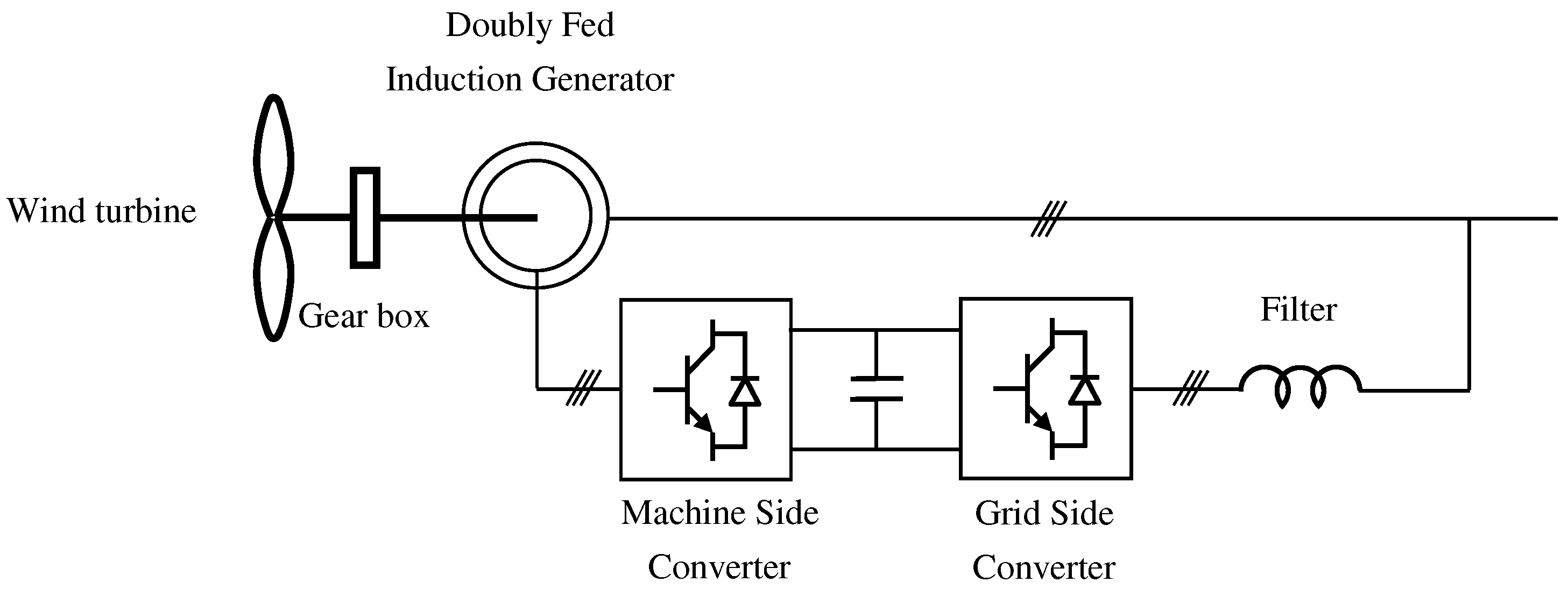
The second generation of WGs (type 3) was based on doubly fed induction generators (DFIGs) with speed control in such a way that the wind turbine runs at the maximum efficiency operating point. DFIGs make use of voltage-source back-to-back power electronic converters that deal with a small fraction of machine rating. Two-pole machines, coupled to the wind turbine through a gearbox, are still used. Today, type 3 wind technology dominates onshore wind generation.

The third generation of WGs (type 4) is based on multi-pole synchronous generators (MSGs). Multi-pole synchronous generators avoid the gearbox that connects the wind turbine and the induction machine in SCIGs and DFIGs. MSGs use voltage-source back-to-back power electronic converters that deal with the whole machine rating. Either constant external field excitation or permanent magnets are used. Today, type 4 wind technology dominates offshore wind generation.

The paper is organized as follows: Section 2, Section 3 and Section 4 contain the detailed models of type 1, 3, and 4 WGs. Section 5 details the general structure of the linear model of a WG. Section 6 proposes tools to identify dynamic patterns in linear dynamic systems. Section 7 investigates the dynamic patterns encountered in power systems with wind generation. Section 8 assesses the impact of the penetration of wind generation on power system small signal stability. Section 9 offers the conclusions of the paper. The Appendix A contains generator data used in the eigenvalue analysis carried out.

2. Model of Type 1 WGs

The general non-linear model of an induction machine in direct and quadrature axes rotating at synchronous speed [13] is governed by a set of differential and algebraic equations that can be grouped into three subsystems.

• Stator windings:

$$\begin{array}{l}\frac{d}{dt}\left[\begin{array}{c}{\psi }_{sd}\\ {\psi }_{sq}\end{array}\right]=-{\omega }_0\left[\begin{array}{cc}{R}_s& 0\\ 0& R_s\end{array}\right]\left[\begin{array}{c}{i}_{sd}\\ i_{sq}\end{array}\right]-{\omega }_0{\omega }_s\left[\begin{array}{cc}0& -1\\ 1& 0\end{array}\right]\left[\begin{array}{c}{\psi }_{sd}\\ {\psi }_{sq}\end{array}\right]+{\omega }_0\left[\begin{array}{c}{v}_{sd}\\ v_{sd}\end{array}\right]\\ \left[\begin{array}{c}{\psi }_{sd}\\ {\psi }_{sq}\end{array}\right]=\left[\begin{array}{cc}{L}_{ss}& 0\\ 0& L_{ss}\end{array}\right]\left[\begin{array}{c}{i}_{sd}\\ i_{sq}\end{array}\right]+\left[\begin{array}{cc}{L}_m& 0\\ 0& L_m\end{array}\right]\left[\begin{array}{c}{i}_{rd}\\ i_{rq}\end{array}\right]\end{array}$$

(1)

• Rotor windings:

$$\begin{array}{l}\frac{d}{dt}\left[\begin{array}{c}{\psi }_{rd}\\ {\psi }_{rq}\end{array}\right]=-{\omega }_0\left[\begin{array}{cc}{R}_r& 0\\ 0& R_r\end{array}\right]\left[\begin{array}{c}{i}_{rd}\\ i_{rq}\end{array}\right]-{\omega }_{0}s{\omega }_s\left[\begin{array}{cc}0& -1\\ 1& 0\end{array}\right]\left[\begin{array}{c}{\psi }_{rd}\\ {\psi }_{rq}\end{array}\right]+{\omega }_0\left[\begin{array}{c}{v}_{rd}\\ v_{rd}\end{array}\right]\\ \left[\begin{array}{c}{\psi }_{rd}\\ {\psi }_{rq}\end{array}\right]=\left[\begin{array}{cc}{L}_m& 0\\ 0& L_m\end{array}\right]\left[\begin{array}{c}{i}_{sd}\\ i_{sq}\end{array}\right]+\left[\begin{array}{cc}{L}_{rr}& 0\\ 0& L_{rr}\end{array}\right]\left[\begin{array}{c}{i}_{rd}\\ i_{rq}\end{array}\right]\end{array}$$

(2)

• Rotor:

  $$\begin{array}{l}2H{\omega }_s\frac{ds}{dt}=t_m-t_e\\ t_e={\psi }_{qr}{i}_{dr}-{\psi }_{dr}{i}_{qr}\end{array}$$

  (3)

  where
  • $v_{sd},v_{sq}$: d- and q-axis components of stator voltage.
  • $v_{rd},v_{rq}$: d- and q-axis components of rotor voltage.
  • $i_{sd},i_{sq}$: d- and q-axis components of stator current.
  • $i_{rd},i_{rq}$: d- and q-axis components of rotor current.
  • ${\psi }_{sd},{\psi }_{sq}$: d- and q-axis components of stator flux.
  • ${\psi }_{rd},{\psi }_{rq}$: d- and q-axis components of rotor flux.
  • $R_s$, $R_r$: stator and rotor resistances.
  • $L_s$, $L_r$: stator and rotor leakage inductance.
  • $L_m$: magnetizing reactance.
  • ${\omega }_0$: speed base ${\omega }_0=2\pi f_0$.
  • $f_0$: fundamental frequency.
  • ${\omega }_s$: synchronous speed ${\omega }_s=1$.
  • $s$: slip.
  • $t_m$: mechanical torque.
  • $t_e$: electromagnetic torque.

Figure 1 shows the equivalent circuit of the induction machine with the criteria adopted. Bold letters in Figure 1 correspond to complex variables. The rotor windings of squirrel cage machines are short-circuited. Hence

$$v_{rd}=v_{rq}=0$$

(4)

The general model of a type 1 WG can be reduced by assuming that the derivatives of the components of the stator fluxes are zero. In other words, we assume that the dynamics of the stator fluxes are much faster than the dynamics of the rotor fluxes and the rotor. Therefore, the set of no linear differential and algebraic Equations (1)–(3) can be written in compact form as

$$\begin{array}{l}\dot{x}=f\left(x,z,\mathbf{\upsilon },u\right)\\ 0=g\left(x,z,\mathbf{\upsilon },u\right)\end{array}$$

(5)

where $x$, $z$, and $\mathbf{\upsilon }$ are, respectively, the vectors of state, algebraic, and stator voltages, and $u$ is the input variable

$$x^T=\left[{\psi }_{rd} {\psi }_{rq} s\right]$$

$$z^T=\left[i_{sd} i_{sq} i_{rd} i_{rq} t_e {\psi }_{sd} {\psi }_{sq}\right]$$

$${\mathbf{\upsilon }}^T=\left[v_{sd} v_{sq}\right]$$

$$u=t_m$$

3. Model of Type 3 WGs

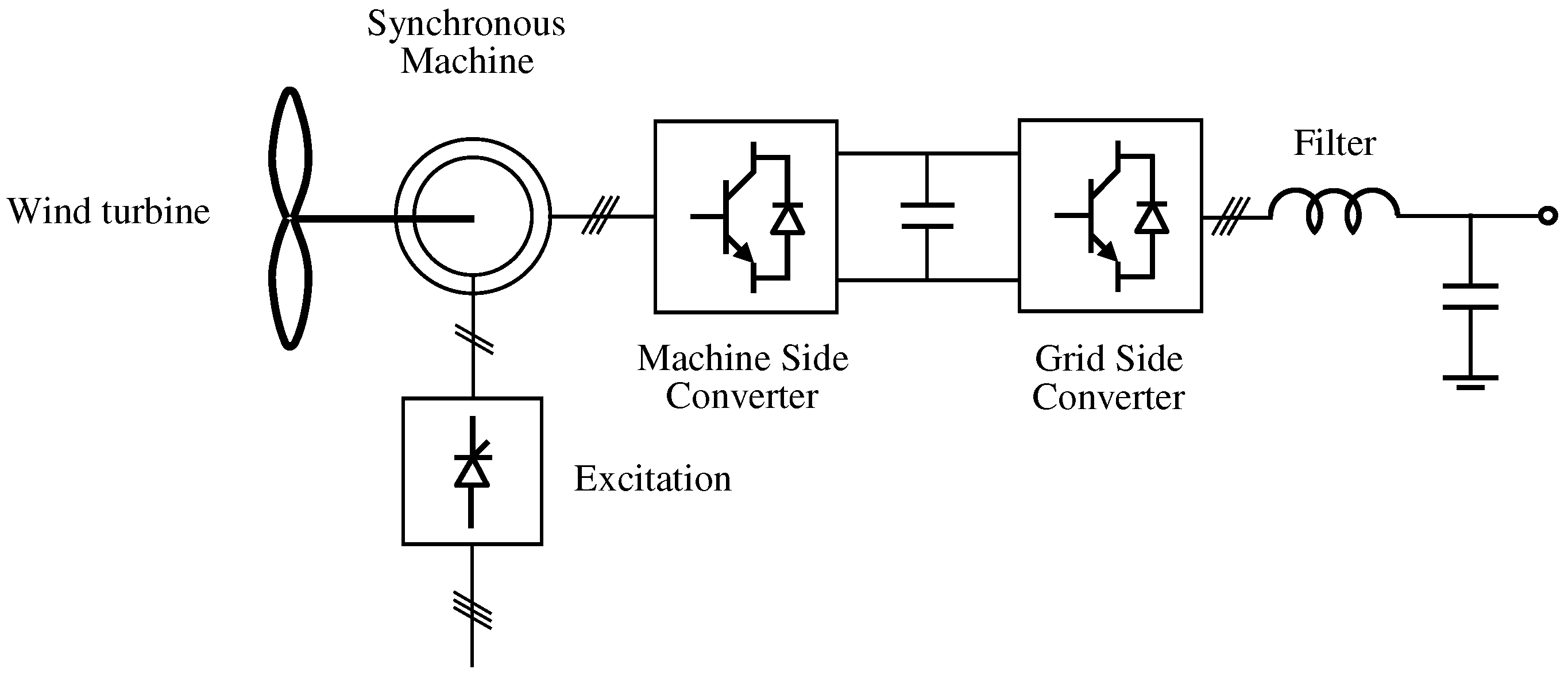
Figure 2 displays the control scheme of a DFIG [14]. The rotor windings are fed by a three-phase voltage-source back-to-back converter. The back-to-back converter is made of two converters coupled through a DC link capacitor: the machine side converter (MSC) and the grid side converter (GSC). The MSC applies a variable-frequency-three-phase voltage system to the rotor windings. The variation in the frequency of the rotor winding voltages results in a variation in the rotor speed. Provided that the stator frequency $f_1$ is constant, a variation in the rotor frequency $f_2$ results in a change in rotor speed $n$ according to:

$$s=\frac{n_1-n}{n_1}=\frac{f_2}{f_1}$$

(6)

The electronic converter is built of two converters coupled through a DC link capacitor, as shown in Figure 2.

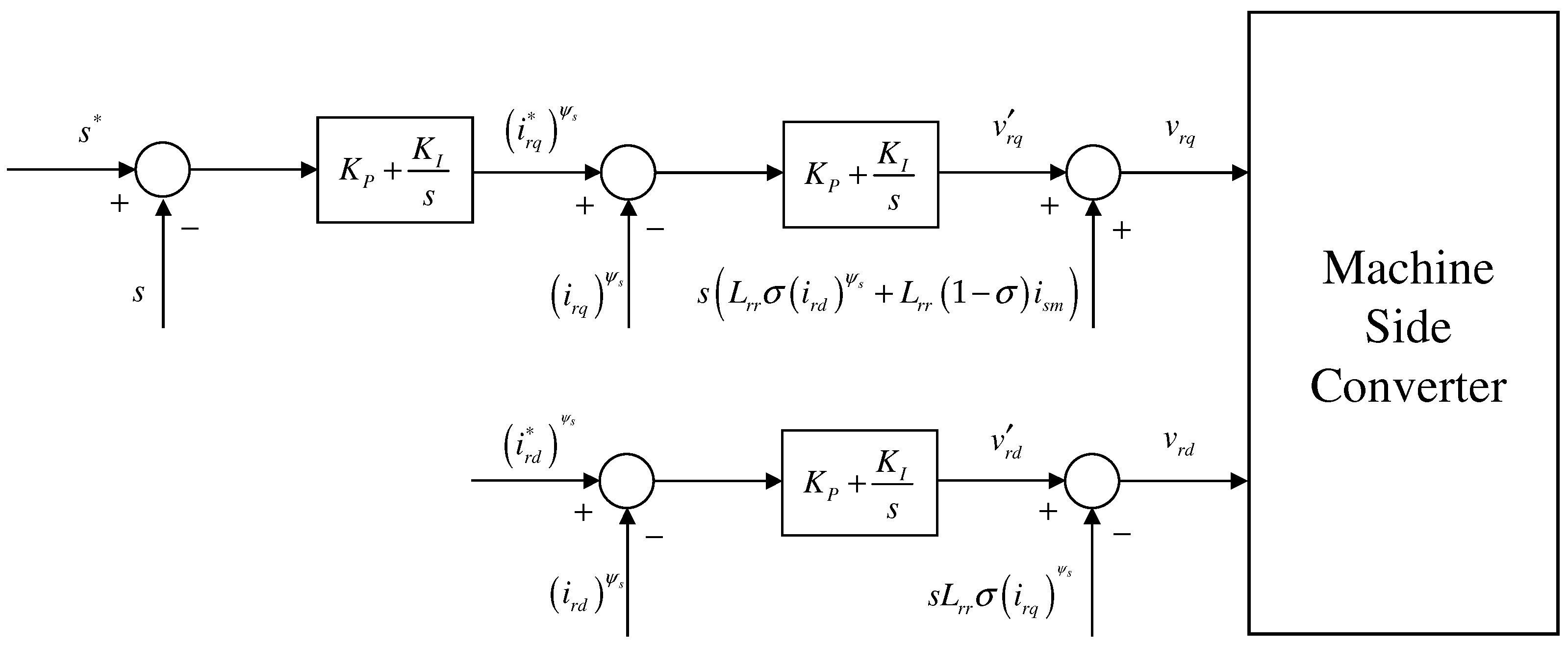
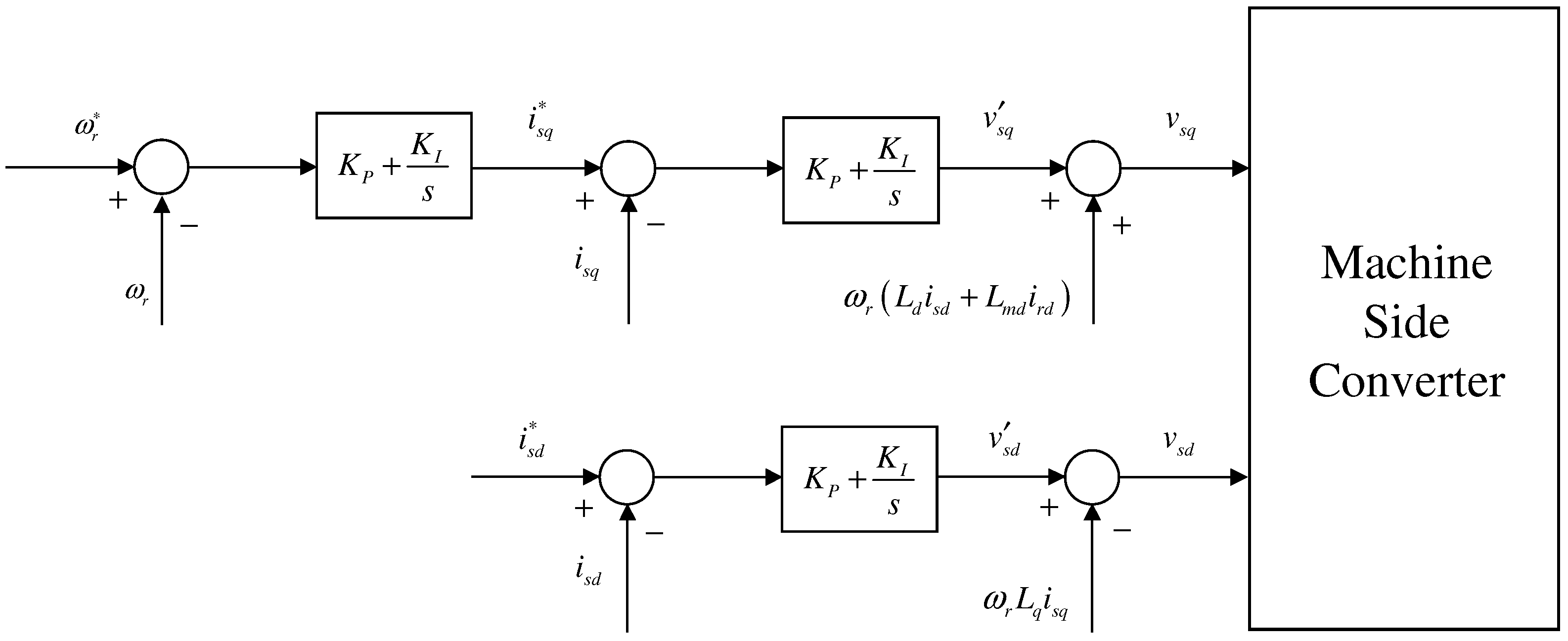
The MSC controls both the torque and the rotor reactive power. The machine magnetizing current component is the direct-axis component of the rotor current in a reference system with the stator flux. The machine excitation current component controls the machine’s reactive power. One possible strategy is to set it equal to zero. This is the one adopted in this paper. The machine torque current component is the quadrature-axis component of rotor current in a reference system solid with stator flux. It controls the electromagnetic torque. The control loops of the MSC are shown in Figure 3. The inner control loops control the rotor current components. An outer control loop controls the rotor speed.

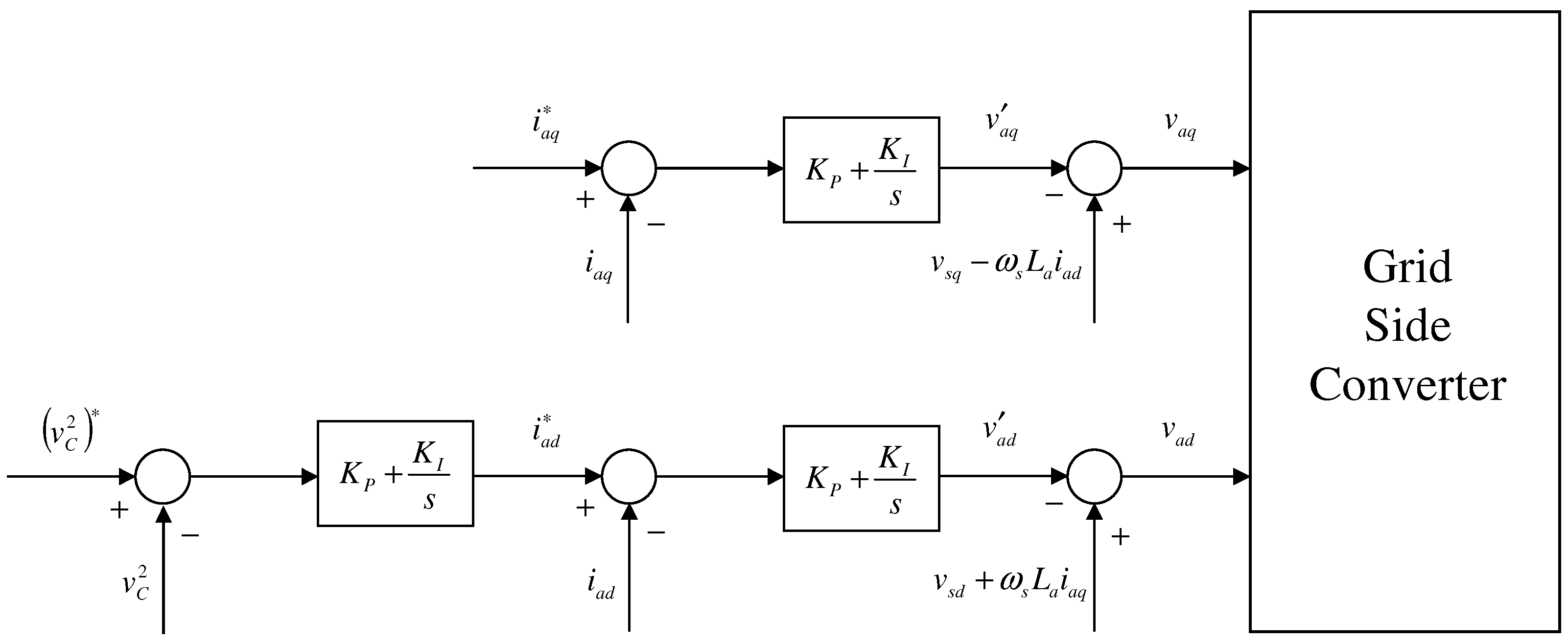
The GSC controls the overall generator reactive power and the DC link capacitor voltage. The power balance in the DC link capacitor governs its voltage. The power balance in the DC link capacitor can be controlled through the direct-axis component of the GSC current. The quadrature-axis component of GSC current controls the reactive power supplied by the GSC. The control loops of the GSC are shown in Figure 4. The inner control loops control the filter-current components. An outer control loop controls the DC link capacitor voltage.

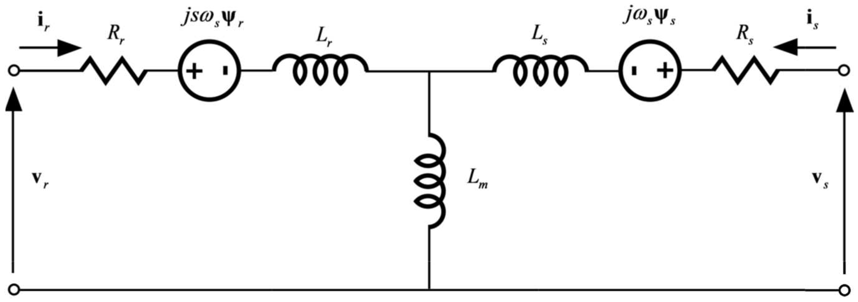
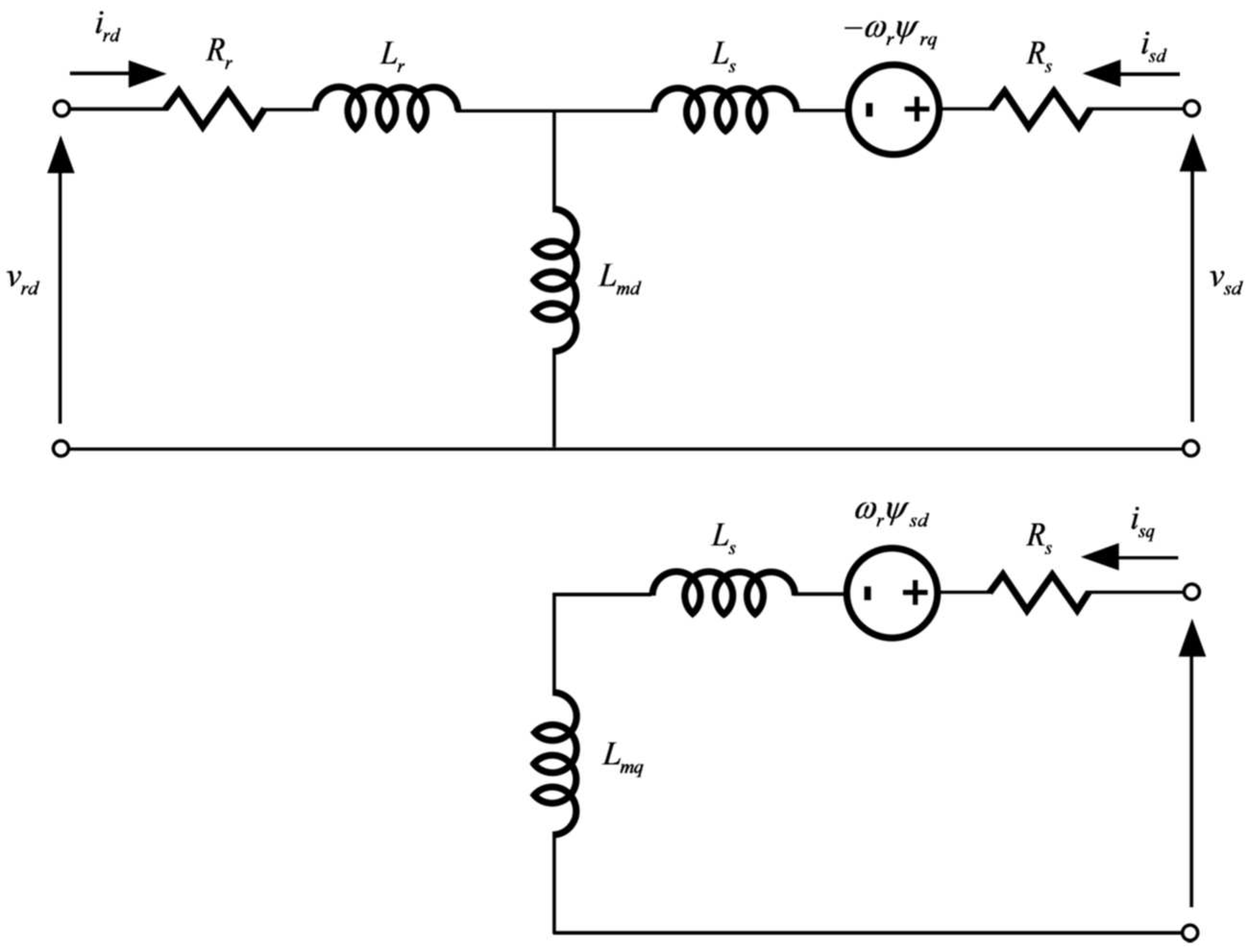
According to the equivalent circuit in Figure 5, the differential-algebraic equations that describe the model of a type 3 WG can be written as a set of differential and algebraic equations that can be grouped into seven groups.

• Machine stator windings:

$$\begin{array}{l}\frac{d}{dt}\left[\begin{array}{c}{\psi }_{sd}\\ {\psi }_{sq}\end{array}\right]=-{\omega }_0\left[\begin{array}{cc}{R}_s& 0\\ 0& R_s\end{array}\right]\left[\begin{array}{c}{i}_{sd}\\ i_{sq}\end{array}\right]-{\omega }_0{\omega }_s\left[\begin{array}{cc}0& -1\\ 1& 0\end{array}\right]\left[\begin{array}{c}{\psi }_{sd}\\ {\psi }_{sq}\end{array}\right]+{\omega }_0\left[\begin{array}{c}{v}_{sd}\\ v_{sd}\end{array}\right]\\ \left[\begin{array}{c}{\psi }_{sd}\\ {\psi }_{sq}\end{array}\right]=\left[\begin{array}{cc}{L}_{ss}& 0\\ 0& L_{ss}\end{array}\right]\left[\begin{array}{c}{i}_{sd}\\ i_{sq}\end{array}\right]+\left[\begin{array}{cc}{L}_m& 0\\ 0& L_m\end{array}\right]\left[\begin{array}{c}{i}_{rd}\\ i_{rq}\end{array}\right]\end{array}$$

(7)

• Grid-side converter:

$$\begin{array}{l}\frac{d}{dt}\left[\begin{array}{c}{\psi }_{ad}\\ {\psi }_{aq}\end{array}\right]=-{\omega }_0\left[\begin{array}{cc}{R}_a& 0\\ 0& R_a\end{array}\right]\left[\begin{array}{c}{i}_{ad}\\ i_{aq}\end{array}\right]\\ -{\omega }_0{\omega }_s\left[\begin{array}{cc}0& -1\\ 1& 0\end{array}\right]\left[\begin{array}{c}{\psi }_{ad}\\ {\psi }_{aq}\end{array}\right]+{\omega }_0\left[\begin{array}{c}{v}_{sd}\\ v_{sq}\end{array}\right]-{\omega }_0\left[\begin{array}{c}{v}_{ad}\\ v_{ad}\end{array}\right]\\ \left[\begin{array}{c}{\psi }_{ad}\\ {\psi }_{aq}\end{array}\right]=\left[\begin{array}{cc}{L}_a& 0\\ 0& L_a\end{array}\right]\left[\begin{array}{c}{i}_{ad}\\ i_{aq}\end{array}\right]\end{array}$$

(8)

• Rotor:

$$\begin{array}{l}\frac{ds}{dt}=\frac{1}{2H{\omega }_s}\left(t_m-t_e\right)\\ t_e={\psi }_{qr}{i}_{dr}-{\psi }_{dr}{i}_{qr}\end{array}$$

(9)

• DC link capacitor:

$$\begin{array}{l}\frac{d\left(v_C^2\right)}{dt}=\frac{2}{C}\left(p_r-p_a\right)\\ p_r=v_{rd}{i}_{rd}+v_{rq}{i}_{rq}\\ p_a=v_{ad}{i}_{ad}+v_{aq}{i}_{aq}\end{array}$$

(10)

• Control of the grid-side converter:

$$\begin{array}{l}{\dot{x}}_{a1}=K_I\left(i_{aq}^{*}-i_{aq}\right)\\ {v^{\prime }}_{aq}=x_{a1}+K_P\left(i_{aq}^{*}-i_{aq}\right)+v_{sq}\\ v_{aq}=-{v^{\prime }}_{aq}-{\omega }_s{L}_a{i}_{ad}\\ {\dot{x}}_{a2}=K_I\left(i_{ad}^{*}-i_{ad}\right)\\ {v^{\prime }}_{ad}=x_{a2}+K_P\left(i_{ad}^{*}-i_{ad}\right)\\ v_{ad}=-{v^{\prime }}_{ad}+{\omega }_s{L}_a{i}_{aq}+v_{sd}\\ {\dot{x}}_{a3}=K_I\left({\left(v_C^2\right)}^{*}-v_C^2\right)\\ i_{ad}^{*}=x_{a3}+K_P\left({\left(v_C^2\right)}^{*}-v_C^2\right)\end{array}$$

(11)

• Machine rotor windings:

$$\begin{array}{l}\frac{d}{dt}\left[\begin{array}{c}{\psi }_{rd}\\ {\psi }_{rq}\end{array}\right]=-{\omega }_0\left[\begin{array}{cc}{R}_r& 0\\ 0& R_r\end{array}\right]\left[\begin{array}{c}{i}_{rd}\\ i_{rq}\end{array}\right]\\ -{\omega }_{0}s{\omega }_s\left[\begin{array}{cc}0& -1\\ 1& 0\end{array}\right]\left[\begin{array}{c}{\psi }_{rd}\\ {\psi }_{rq}\end{array}\right]+{\omega }_0\left[\begin{array}{c}{v}_{rd}\\ v_{rd}\end{array}\right]\\ \left[\begin{array}{c}{\psi }_{rd}\\ {\psi }_{rq}\end{array}\right]=\left[\begin{array}{cc}{L}_m& 0\\ 0& L_m\end{array}\right]\left[\begin{array}{c}{i}_{sd}\\ i_{sq}\end{array}\right]+\left[\begin{array}{cc}{L}_{rr}& 0\\ 0& L_{rr}\end{array}\right]\left[\begin{array}{c}{i}_{rd}\\ i_{rq}\end{array}\right]\end{array}$$

(12)

• Machine-side converter:

  $$\begin{array}{l}{\dot{x}}_1=K_I\left({\left(i_{rd}^{*}\right)}^{{\psi }_s}-{\left(i_{rd}\right)}^{{\psi }_s}\right)\\ {v^{\prime }}_{rd}=x_1+K_P\left({\left(i_{rd}^{*}\right)}^{{\psi }_s}-{\left(i_{rd}\right)}^{{\psi }_s}\right)\\ {\left(v_{rd}\right)}^{{\psi }_s}={v^{\prime }}_{rd}-s{\omega }_s{L}_{rr}\sigma {\left(i_{rq}\right)}^{{\psi }_s}\\ {\dot{x}}_2=K_I\left({\left(i_{rq}^{*}\right)}^{{\psi }_s}-{\left(i_{rq}\right)}^{{\psi }_s}\right)\\ {v^{\prime }}_{rq}=x_2+K_P\left({\left(i_{rq}^{*}\right)}^{{\psi }_s}-{\left(i_{rq}\right)}^{{\psi }_s}\right)\\ {\left(v_{rq}\right)}^{{\psi }_s}={v^{\prime }}_{rq}+s{\omega }_s\left(L_{rr}\sigma {\left(i_{rd}\right)}^{{\psi }_s}+L_{rr}\left(1-\sigma \right)i_{sm}\right)\\ {\dot{x}}_3=K_I\left(s^{*}-s\right)\\ {\left(i_{rq}^{*}\right)}^{{\psi }_s}=x_3+K_P\left(s^{*}-s\right)\end{array}$$

  (13)

  $$\begin{array}{l}{i}_{sm}=\frac{{\psi }_s}{L_m}\hfill \\ {\psi }_s=\sqrt{{\psi }_{sd}^2+{\psi }_{sq}^2}\hfill \end{array}$$

  (14)

  $$\begin{array}{l}\varphi =\arctan \frac{{\psi }_{sd}}{{\psi }_{sq}}\\ \left[\begin{array}{c}{v}_{rd}\\ v_{rq}\end{array}\right]=\left[\begin{array}{cc}\cos \varphi & -\sin \varphi \\ \sin \varphi & \cos \varphi \end{array}\right]{\left[\begin{array}{c}{v}_{rd}\\ v_{rq}\end{array}\right]}^{{\psi }_s}\\ \left[\begin{array}{c}{i}_{rd}\\ i_{rq}\end{array}\right]=\left[\begin{array}{cc}\cos \varphi & -\sin \varphi \\ \sin \varphi & \cos \varphi \end{array}\right]{\left[\begin{array}{c}{i}_{rd}\\ i_{rq}\end{array}\right]}^{{\psi }_s}\end{array}$$

  (15)

  where:
  • $v_{ad},v_{aq}$: d- and q-axis components of rotor-side filter voltage.
  • $i_{ad},i_{aq}$: d- and q-axis components of grid-side filter current.
  • ${\psi }_{ad},{\psi }_{aq}$: d- and q-axis components of grid-side filter flux.
  • $R_a$, $L_a$: resistance and inductance of a grid-side filter.
  • $v_C$: DC link capacitor voltage.
  • $C$: capacitance of a DC link capacitor.
  • $x_{a1},x_{a2},x_{a3}$: state variables that describe the PI controllers of the grid side converter.
  • $x_1,x_2,x_3$: state variables that describe the PI controllers of the machine side converter.
  • $K_P,K_I$: parameters of the PI regulators (the values of the parameters of the PI regulators depend on the loop).
  • ${\left[·\right]}^{\ast }$: reference value of $\left[·\right]$.

The general model of a type 3 WG is simplified, assuming that the dynamics of the components of the stator flux are negligible [15]. Hence, the set of no linear differential and algebraic Equations (7)–(15) can be written in compact form as:

$$\begin{array}{l}\dot{x}=f\left(x,z,\mathbf{\upsilon },u\right)\\ 0=g\left(x,z,\mathbf{\upsilon },u\right)\end{array}$$

(16)

where $x$, $z$, $\mathbf{\upsilon }$ and $u$ are, respectively, the vectors of state, algebraic, stator voltages, and input variables:

$$x^T=\left[{\psi }_{sd} {\psi }_{sq} {\psi }_{rd} {\psi }_{rq} {\psi }_{ad} {\psi }_{aq} s v_C^2 x_{a1} x_{a2} x_{a3} x_{r1} x_{r2} x_s\right]$$

$${\mathbf{\upsilon }}^T=\left[v_{sd} v_{sq}\right]$$

$$\begin{array}{l}{z}^T=\left[{\psi }_{sd} {\psi }_{sq} i_{sd} i_{sq} i_{rd} i_{rq} i_{ad} i_{aq} v_{ad} v_{aq} i_{ad}^{*} i_{sm} {\psi }_s \varphi \right.\\ \left.{\left(v_{rd}\right)}^{{\psi }_s} {\left(v_{rq}\right)}^{{\psi }_s} v_{rd} v_{rd} {\left(i_{rd}\right)}^{{\psi }_s} {\left(i_{rq}\right)}^{{\psi }_s} t_e p_r p_a {\left(i_{rq}^{*}\right)}^{{\psi }_s}\right]\end{array}$$

$$u=\left[t_m i_{aq}^{*} v_C^{*} {\left(i_{rd}^{*}\right)}^{{\psi }_s} s^{*}\right]$$

4. Model of a Type 4 WG

Figure 6 displays the control scheme of a MSG ([16,17]). The machine stator windings are fed by a three-phase voltage source back-to-back converter. The back-to-back converter is made of two converters coupled through a DC link capacitor: the machine side converter (MSC) and the grid side converter (GSC). The MSC applies to the stator windings in a three-phase voltage system of variable frequency. The variation in the frequency of machine stator voltages results in a variation in the rotor speed.

The MSC is used to control either the torque or the rotor. The component in the quadrature axis of the stator current controls the electromagnetic torque when the component in the direct axis of the stator current is equal to zero. shows the controllers of the MSC. The control loops of the MSC are shown in Figure 7. The inner control loops control the stator current components. An outer control loop controls the rotor speed.

The control philosophy of the GSC of a type 4 WG is identical to the control philosophy of a type 3 WG. Hence, the block diagrams in Figure 4 are fully applicable to type 4 WGs.

The equations that describe the model of a type 4 WG can be written as a set of differential and algebraic equations that can be grouped into six groups [16,17,18].

Stator windings (see Figure 8):

$$\begin{array}{l}\frac{d}{dt}\left[\begin{array}{c}{\psi }_{sd}\\ {\psi }_{sq}\end{array}\right]=-{\omega }_0\left[\begin{array}{cc}{R}_s& 0\\ 0& R_s\end{array}\right]\left[\begin{array}{c}{i}_{sd}\\ i_{sq}\end{array}\right]-{\omega }_0{\omega }_r\left[\begin{array}{cc}0& -1\\ 1& 0\end{array}\right]\left[\begin{array}{c}{\psi }_{sd}\\ {\psi }_{sq}\end{array}\right]+{\omega }_0\left[\begin{array}{c}{v}_{sd}\\ v_{sd}\end{array}\right]\\ \left[\begin{array}{c}{\psi }_{sd}\\ {\psi }_{sq}\end{array}\right]=\left[\begin{array}{cc}{L}_d& 0\\ 0& L_q\end{array}\right]\left[\begin{array}{c}{i}_{sd}\\ i_{sq}\end{array}\right]+\left[\begin{array}{c}{L}_{md}\\ 0\end{array}\right]i_{rd}\end{array}$$

(17)

• Grid-side converter:

$$\begin{array}{l}\frac{d}{dt}\left[\begin{array}{c}{\psi }_{ad}\\ {\psi }_{aq}\end{array}\right]=-{\omega }_0\left[\begin{array}{cc}{R}_a& 0\\ 0& R_a\end{array}\right]\left[\begin{array}{c}{i}_{ad}\\ i_{aq}\end{array}\right]\\ -{\omega }_0{\omega }_s\left[\begin{array}{cc}0& -1\\ 1& 0\end{array}\right]\left[\begin{array}{c}{\psi }_{ad}\\ {\psi }_{aq}\end{array}\right]+{\omega }_0\left[\begin{array}{c}{v}_{sd}\\ v_{sq}\end{array}\right]-{\omega }_0\left[\begin{array}{c}{v}_{ad}\\ v_{ad}\end{array}\right]\\ \left[\begin{array}{c}{\psi }_{ad}\\ {\psi }_{aq}\end{array}\right]=\left[\begin{array}{cc}{L}_a& 0\\ 0& L_a\end{array}\right]\left[\begin{array}{c}{i}_{ad}\\ i_{aq}\end{array}\right]\end{array}$$

(18)

• Rotor:

$$\begin{array}{l}\frac{d{\omega }_r}{dt}=\frac{1}{2H}\left(t_e-t_m\right)\\ t_e={\psi }_{sd}{i}_{sq}\end{array}$$

(19)

• DC link capacitor:

$$\begin{array}{l}\frac{d\left(v_C^2\right)}{dt}=\frac{2}{C}\left(p_s-p_a\right)\\ p_s=v_{sd}{i}_{sd}+v_{sq}{i}_{sq}\\ p_a=v_{ad}{i}_{ad}+v_{aq}{i}_{aq}\end{array}$$

(20)

• Control of the grid side converter.

$$\begin{array}{l}{\dot{x}}_{a1}=K_{Ia}\left(i_{aq}^{*}-i_{aq}\right)\\ {v^{\prime }}_{aq}=x_{a1}+K_{Pa}\left(i_{aq}^{*}-i_{aq}\right)\\ v_{aq}=v_q-{\omega }_s{L}_a{i}_{ad}-{v^{\prime }}_{aq}\\ {\dot{x}}_{a2}=K_{Ia}\left(i_{ad}^{*}-i_{ad}\right)\\ {v^{\prime }}_{ad}=x_{a2}+K_{Pa}\left(i_{ad}^{*}-i_{ad}\right)\\ v_{ad}=v_d+{\omega }_s{L}_a{i}_{aq}-{v^{\prime }}_{ad}\\ {\dot{x}}_{a3}=K_{Iv}\left({\left(v_C^2\right)}^{*}-v_C^2\right)\\ i_{ad}^{*}=x_{a3}+K_{Pv}\left({\left(v_C^2\right)}^{*}-v_C^2\right)\end{array}$$

(21)

• Control of the machine side converter:

  $$\begin{array}{l}{\dot{x}}_1=K_I\left(i_{sd}^{*}-i_{sd}\right)\\ {v^{\prime }}_{sd}=x_1+K_P\left(i_{sd}^{*}-i_{sd}\right)\\ v_{sd}={v^{\prime }}_{sd}-{\omega }_r{L}_q{i}_{sq}\\ {\dot{x}}_2=K_I\left(i_{sq}^{*}-i_{sq}\right)\\ {v^{\prime }}_{sq}=x_2+K_P\left(i_{sq}^{*}-i_{sq}\right)\\ v_{sq}={v^{\prime }}_{sq}+{\omega }_r\left(L_d{i}_{sd}+L_{md}{i}_{rd}\right)\\ {\dot{x}}_3=K_I\left({\omega }_r^{*}-{\omega }_r\right)\\ i_{sq}^{*}=x_3+K_P\left({\omega }_r^{*}-{\omega }_r\right)\end{array}$$

  (22)

  where:
  • $L_d$, $L_q$: d- and q-axis synchronous inductance.
  • $L_{md}$, $L_{mq}$: d- and q-axis magnetizing reactance.

The set of no linear differential and algebraic Equations (17)–(22) can be written in compact form as:

$$\begin{array}{l}\dot{x}=f\left(x,z,\mathbf{\upsilon },u\right)\\ 0=g\left(x,z,\mathbf{\upsilon },u\right)\end{array}$$

(23)

where $x$, $z$, $\mathbf{\upsilon }$ and $u$ are, respectively, the vectors of state, algebraic, stator voltages, and input variables:

$$x^T=\left[{\psi }_{sd} {\psi }_{sq} {\psi }_{ad} {\psi }_{aq} v_C^2 x_{a1} x_{a2} x_{a3} x_{s1} x_{s2} {\omega }_r x_{{\omega }_r}\right]$$

$$z^T=\left[i_{sd}{i}_{sq}{i}_{ad} i_{aq} v_{ad} v_{aq} v_{sd}{v}_{sq}{v^{\prime }}_{sd} {v^{\prime }}_{sq} i_{ad}^{*} t_e p_s p_a{i}_{sq}^{*}\right]$$

$${\mathbf{\upsilon }}^T=\left[v_d v_q\right]$$

$$u^T=\left[t_m i_{rd} i_{aq}^{*} {\left(v_C^2\right)}^{*} i_{sd}^{*} {\omega }_r^{*}\right]$$

5. Linear Models of WGs

The linear model of a WG is obtained by linearizing the set of non-linear differential and algebraic equations.

$$\begin{array}{c}\dot{x}-{\dot{x}}_0={\left.\frac{\partial f\left(x,z,\mathbf{\upsilon },u\right)}{\partial x}\right|}_{x=x_0,z=z_0,\mathbf{\upsilon }={\mathbf{\upsilon }}_0,u=u_0}\left(x-x_0\right)\\ +{\left.\frac{\partial f\left(x,z,\mathbf{\upsilon },u\right)}{\partial z}\right|}_{x=x_0,z=z_0,\mathbf{\upsilon }={\mathbf{\upsilon }}_0,u=u_0}\left(z-z_0\right)\\ +{\left.\frac{\partial f\left(x,z,\mathbf{\upsilon },u\right)}{\partial u}\right|}_{x=x_0,z=z_0,\mathbf{\upsilon }={\mathbf{\upsilon }}_0,u=u_0}\left(\mathbf{\upsilon }-{\mathbf{\upsilon }}_0\right)\\ +{\left.\frac{\partial f\left(x,z,\mathbf{\upsilon },u\right)}{\partial u}\right|}_{x=x_0,z=z_0,\mathbf{\upsilon }={\mathbf{\upsilon }}_0,u=u_0}\left(u-u_0\right)\end{array}$$

(24)

$$\begin{array}{c}0={\left.\frac{\partial g\left(x,z,\mathbf{\upsilon },u\right)}{\partial x}\right|}_{x=x_0,z=z_0,\mathbf{\upsilon }={\mathbf{\upsilon }}_0,u=u_0}\left(x-x_0\right)\\ +{\left.\frac{\partial g\left(x,z,\mathbf{\upsilon },u\right)}{\partial z}\right|}_{x=x_0,z=z_0,\mathbf{\upsilon }={\mathbf{\upsilon }}_0,u=u_0}\left(z-z_0\right)\\ +{\left.\frac{\partial g\left(x,z,\mathbf{\upsilon },u\right)}{\partial u}\right|}_{x=x_0,z=z_0,\mathbf{\upsilon }={\mathbf{\upsilon }}_0,u=u_0}\left(\mathbf{\upsilon }-{\mathbf{\upsilon }}_0\right)\\ +{\left.\frac{\partial g\left(x,z,\mathbf{\upsilon },u\right)}{\partial u}\right|}_{x=x_0,z=z_0,\mathbf{\upsilon }={\mathbf{\upsilon }}_0,u=u_0}\left(u-u_0\right)\end{array}$$

on in a more compact form:

$$\begin{array}{l}\left[\begin{array}{c}\Delta \dot{x}\\ 0\\ 0\end{array}\right]=\left[\begin{array}{ccc}{A}_{11}& A_{12}& A_{13}\\ A_{21}& A_{22}& A_{32}\\ A_{31}& A_{32}& A_{33}\end{array}\right]\left[\begin{array}{c}\Delta x\\ \Delta z\\ \Delta \mathbf{\upsilon }\end{array}\right]+\left[\begin{array}{c}{B}_1\\ B_2\\ B_3\end{array}\right]\Delta u\\ \Delta i=\left[\begin{array}{ccc}0& C_2& 0\end{array}\right]\left[\begin{array}{c}\Delta x\\ \Delta z\\ \Delta \mathbf{\upsilon }\end{array}\right]\end{array}$$

(25)

The linear model of a WG for small-signal stability analysis of a power system is obtained by eliminating the algebraic variables from (25):

$$\begin{array}{l}\Delta \dot{x}=A\Delta x+B_{\mathbf{\upsilon }}\Delta \mathbf{\upsilon }+B_u\Delta u\\ \Delta i=C\Delta x+D_{\mathbf{\upsilon }}\Delta \mathbf{\upsilon }+D_u\Delta u\end{array}$$

(26)

The model of the electrical grid is described by a set of algebraic equations that relate the voltage variables with the current variables:

$$\Delta i=J\Delta \mathbf{\upsilon }$$

(27)

The overall power system model is built by incorporating (27) to (26):

$$\Delta \dot{x}=\left[A+B_{\mathbf{\upsilon }}{\left(J-D_{\mathbf{\upsilon }}\right)}^{-1}C\right]\Delta x+\left[D_u+B_u{\left(J-D_{\mathbf{\upsilon }}\right)}^{-1}{D}_u\right]\Delta u$$

(28)

6. Identifying Dynamic Patterns in Linear Dynamic Systems

Dynamic patterns are close associations between state variables and eigenvalues of the linear model of a dynamic system. Participation factors developed in the context of Selective Modal Analysis [19] have become standard tools for identifying the relationships between eigenvalues and state variables [20].

Let us consider an undriven linear dynamic system described by a set of linear first-order differential equations:

$$\begin{array}{c}\Delta \dot{x}=A\Delta x\\ A\in {\Re }^{N\times N}\end{array}$$

(29)

The solution of the set of linear differential Equation (29) provides the response of the linearized dynamic system to initial conditions different from zero. Such a solution depends on the exponential of the state matrix $A$ according to:

$$\Delta x=e^{At}\Delta x\left(0\right)$$

(30)

A meaningful approach to computing the exponential of the state matrix $A$ is based on its eigenvalues and eigenvectors. An eigenvalue ${\lambda }_i$ of the state matrix $A$ and the associated right $v_i$ and left $w_i$ eigenvectors are defined as:

$$A{v}_i=v_i{\lambda }_i$$

(31)

$$w_i^{T}A={\lambda }_i{w}_i^T$$

(32)

The study of Equations (31) and (32) indicates that the right and left eigenvectors are not uniquely determined (they are computed as the solutions of a linear system of N equations and N + 1 unknowns). An approach to eliminating that degree of freedom is to introduce a normalization such as:

$$w_i^T{v}_i=1$$

(33)

In the case of N distinct eigenvalues, Equations (31)–(33) can be written together for all eigenvalues in matrix form as:

$$\begin{array}{c}AV=V\mathbf{\Lambda }\\ WA=\mathbf{\Lambda }W\\ WV=I\end{array}$$

(34)

where $\mathbf{\Lambda }$, $V$ y $W$ are, respectively, the matrices of eigenvalues and right and left eigenvectors:

$$\begin{array}{c}\mathbf{\Lambda }=\left[\begin{array}{ccc}{\lambda }_1& & \\ & \ddots & \\ & & {\lambda }_N\end{array}\right]\\ V=\left[\begin{array}{ccc}{v}_1& \cdots & v_N\end{array}\right]\\ W=\left[\begin{array}{c}{w}_1^T\\ ⋮\\ w_N^T\end{array}\right]\end{array}$$

If the exponential of the state matrix $e^{At}$ is expressed in terms of eigenvalues and right and left eigenvectors of the state matrix (34), Equation (30):

$$\Delta x=V{e}^{\mathbf{\Lambda }t}W\Delta x\left(0\right)={\displaystyle \sum _{i=1}^N{v}_i}{e}^{{\lambda }_{i}t}\left[w_i^T\Delta x\left(0\right)\right]$$

(35)

The study of Equation (35) allows drawing the following conclusions:

• The system response is expressed as the combination of the system response for N modes.
• The eigenvalues of the state matrix determine the system’s stability. A real negative (positive) eigenvalue indicates exponentially decreasing (increasing) behavior. A complex eigenvalue of the negative (positive) real part indicates oscillatory decreasing (increasing) behavior.
• The components of the right eigenvector $v_i$ indicate the relative activity of each variable in the i-th mode.
• The components of the left eigenvector $w_i$ weight the initial conditions (they are the excitations) in the i-th mode.

The participation factor of the j-th variable in the i-th mode is defined as the product of the j-th components of the right $v_{ji}$ and left $w_{ji}$ eigenvectors corresponding to the i-th mode [19]:

$$p_{ji}=w_{ji}{v}_{ji}$$

(36)

The participation factor of a variable in a mode is its nondimensional magnitude. In other words, it is independent of the units of the state variables.

In addition, as a result of the adopted normalization (33), the sum of the participation factors of all variables in a mode and the sum of the participation factors of all modes in a variable are equal to unity.

$${\displaystyle \sum _{j=1}^N{p}_{ji}}={\displaystyle \sum _{i=1}^N{p}_{ji}}=1$$

(37)

The $S$ subsystem participation in the i-th mode is defined as the magnitude of the sum of the participation factors of the variables that describe the subsystem $S$ [21]:

$$p_{Si}=\left|{\displaystyle \sum _{j\in S}{p}_{ji}}\right|$$

(38)

7. Dynamic Patterns in Power Systems with Wind Generation

Our approach to studying the dynamic patterns in power systems with wind generators starts by comparing the eigenvalues of a synchronous generator (SG) connected to an infinite bus with the eigenvalues of a WG (of any type) also connected to an infinite bus. Then, we consider the case of two generators: SG and WG, and investigate the interaction of the two generators in the case of WG using different technologies.

7.1. Single Generator Connected to an Infinite Bus

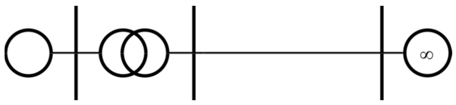
The eigenvalues of the linear model of four models of a single generator (SG, type 1 WG, type 3 WG, or type 4 WG) connected to an infinite bus, according to Figure 9, are firstly detailed and compared. We are precisely interested in learning if WGs exhibit electromechanical oscillations as SGs do.

Table 1. Complex eigenvalues of the model of a synchronous generator connected to an infinite bus.

Complex Eigenvalues
No.	Real (1/s)	Imaginary (rad/s)	Damping (%)	Frequency (Hz)
1, 2	–0.4682	±6.1222	7.62	0.97
3, 4	–0.6560	±0.7209	67.30	0.11
5, 6	–36.6094	±0.1017	100.00	0.02

and

Table 2. Real eigenvalues of the model of a synchronous generator connected to an infinite bus.

Real Eigenvalues
No.	Real (1/s)	Time Constant (s)
7	–0.1421	7.0386
8	–1.6772	0.5962
9	–3.1264	0.3199
10	–4.927	0.2030
11	–10.1524	0.0985
12	–99.7227	0.0100

contain, respectively, the complex and the real eigenvalues of the linear model of an SG connected to an infinite bus. The model of an SG comprises detailed representations of the synchronous machine, the governor turbine, and the excitation system. Table 1 and Table 2 display twelve eigenvalues, as the linear model is described by twelve state variables. There are three complex pairs and six real eigenvalues. All of them lie in the left-half plane, which means that the system is stable. The electromechanical oscillation of the synchronous generator is characterized by the complex pair (1, 2). The electromechanical oscillation is easily identified since the damping of the associated eigenvalue is much lower than the damping of the remaining complex pairs of eigenvalues (7%) and its frequency (1 Hz) is in the frequency range of power system electromechanical oscillations (between 0.1 and 2 Hz).

If a type 1 WG is connected to an infinite bus instead of a SG, the linear model is only described by three state variables.

Table 3. Complex eigenvalues of the model of a type 1 WG connected to an infinite bus.

Complex Eigenvalues
No.	Real (1/s)	Imaginary (rad/s)	Damping (%)	Frequency (Hz)
1, 2	–4.1759	±9.2741	41.06	1.48

and

Table 4. Real eigenvalues of the model of a type 1 WG connected to an infinite bus.

Real Eigenvalues
No.	Real (1/s)	Time Constant (s)
3	–3.719	0.2689

contain, respectively, the complex and the real eigenvalues of the linear model of a type 1 WG connected to an infinite bus. There is one complex pair and one real eigenvalue. All of them lie in the left-half plane, which means that the system is stable. The electromechanical oscillation is characterized by a complex pair. The frequency of the electromechanical oscillation of a type 1 WG is in the range of power system electromechanical oscillations. In contrast, its damping is much higher than the damping of SG electromechanical oscillations.

If a type 3 WG is connected to an infinite bus instead of a type 1 WG, the linear model is described by twelve state variables.

Table 5. Eigenvalues of the model of a type 3 WG connected to an infinite bus.

Complex Eigenvalues
No.	Real (1/s)	Imaginary (rad/s)	Damping (%)	Frequency (Hz)
1, 2	–17.5000	±17.8536	70.00	2.84
3, 4	–8.8205	±16.8485	46.38	2.68
5, 6	–15.5190	±16.2157	69.14	2.58
7, 8	–9.4275	±15.7293	51.41	2.50
9, 10	–1.9406	±1.9075	71.32	0.30
11, 12	–1.6215	±1.8696	65.52	0.30

contains the eigenvalues of the linear model of a type 3 WG connected to an infinite bus. There are six complex pairs. All of them lie in the left-half plane, which means that the system is stable. The frequency of four complex pairs is around 3 Hz, whereas the frequency of the remaining two complex pairs is around 0.3 Hz. The damping of all complex modes is between 40% and 70%. The frequency and damping of system eigenvalues are determined by the design criteria of the control loops of the converter controls [15]. The bandwidth of the inner and outer control loops is 25 rad/s and 2.5 rad/s, respectively. The requested damping of the equivalent second-order system is 70%. It should be noted that the frequency and damping of the eigenvalues of a type 3 WG are not in the range of SG electromechanical oscillations.

The connection of a type 4 WG to an infinite bus is studied as well. The linear model is also described by twelve state variables.

Table 6. Eigenvalues of the model of a type 4 WG connected to an infinite bus.

Complex Eigenvalues
No.	Real (1/s)	Imaginary (rad/s)	Damping (%)	Frequency (Hz)
1, 2	–15.6949	±18.563	64.56	2.95
3, 4	–10.7595	±18.4774	50.32	2.94
5, 6	–17.5000	±17.8536	70.00	2.84
7, 8	–22.3780	±17.723	78.39	2.82
9, 10	–1.8051	±1.8309	70.21	0.29
11, 12	–1.8655	±1.8083	71.80	0.29

displays the eigenvalues of its state matrix. There are six complex pairs lying in the left-half plane, which means that the system is stable. The damping and frequency of the eigenvalues of a type 4 linear model are fairly similar to those of a DFIG one, as they are dictated by the design criteria of the converter controls [18]. Moreover, the frequency and damping of the eigenvalues of a type 4 WG are not in the range of SG electromechanical oscillations.

We have found that type 1 WGs exhibit well-damped oscillations in the upper frequency range of SG electromechanical oscillations. In addition, type 3 and 4 WGs exhibit well-damped oscillations outside the frequency range of the SG electromechanical oscillations due to the design criteria of their converter controls.

7.2. Two Generators Connected to an Infinite Bus

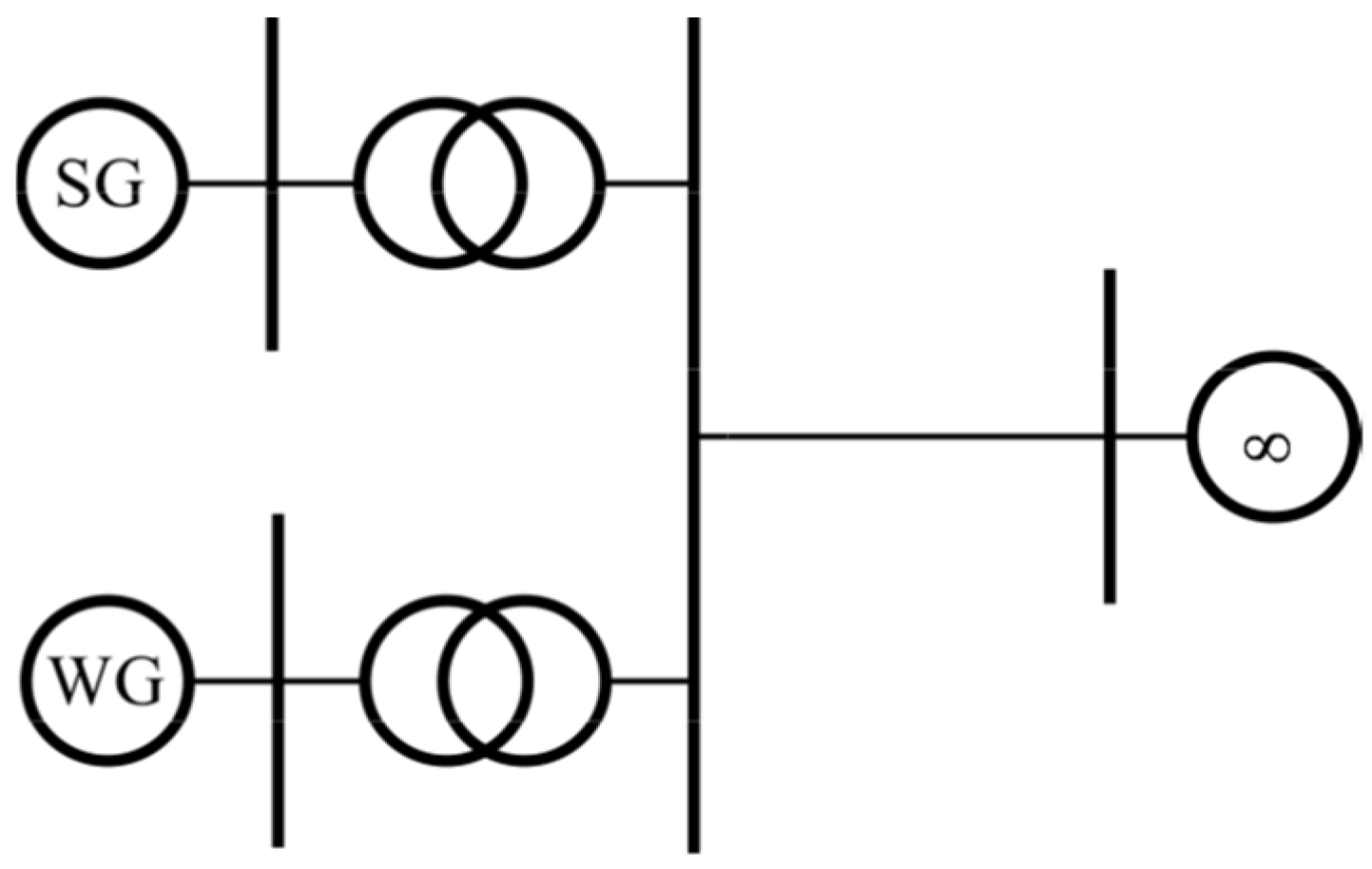
The interaction between SGs and WGs of different technologies is evaluated first, assuming the power system example in Figure 10. Eigenvalues and participation factors of each generator (subsystem participation) in each eigenvalue are used for this purpose. It will be assumed that both generators supply 50% of the total generation delivered to the infinite bus.

Table 7. Complex eigenvalues when both the SG and the type 1 WG supply 50% of the total generation.

Complex Eigenvalues
No.	Real (1/s)	Imaginary (rad/s)	Damping (%)	Frequency (Hz)
1, 2	–5.1143	8.1753	53.04	1.30
3, 4	–0.6037	6.4592	9.31	1.03
5, 6	–0.6062	0.6890	66.06	0.11

and

Table 8. Real eigenvalues when both the SG and the type 1 WG supply 50% of the total generation.

Real Eigenvalues
No.	Real (1/s)	Time Constant (s)
7	–0.1421	7.0358
8	–1.6763	0.5966
9	–2.9954	0.3338
10	–3.1205	0.3205
11	–5.0899	0.1965
12	–10.1434	0.0986
13	–37.3601	0.0268
14	–37.4924	0.0267
15	–99.7556	0.0100

display, respectively, the complex and real eigenvalues when the WG is type 1.

Table 9. Generator participations when both the SG and the type 1 WG supply 50% of the total generation. The generator with greatest participation in each eigenvalue is highlighted in shadow grey.

		Generator
		SG	Type 1 WG
Eigenvalue	1, 2	0.01	1
	3, 4	1	0.01
	5, 6	1	0.01
	7	1	0
	8	1	0
	9	0.1	1.1
	10	1.11	0.11
	11	0.98	0.02
	12	1	0
	13	1	0
	14	1	0
	15	1	0

display the generator participations. The generator with greatest participation in each eigenvalue is highlighted in shadow grey. Participations close to one indicate that the dynamics associated to the eigenvalue of interest are dominated by the corresponding generator. Hence, generator participations clearly indicate that the complex pair of eigenvalues (1, 2) and the real one (9) are associated with the type 1 WG, whereas the remaining ones are associated with the SG.

The interaction between a SG and a type 3 WG is now considered. Complex eigenvalues, real eigenvalues and participation factors, displayed, respectively, in

Table 10. Complex eigenvalues when both the SG and the type 3 WG supply 50% of the total generation.

Complex Eigenvalues
No.	Real (1/s)	Imaginary (rad/s)	Damping (%)	Frequency (Hz)
1, 2	–17.5000	17.8536	70.00	2.84
3, 4	–9.5207	16.8765	49.13	2.69
5, 6	–10.4829	16.4688	53.70	2.62
7, 8	–15.7406	16.4223	69.20	2.61
9, 10	–0.5839	6.4667	8.99	1.03
11, 12	–1.7774	1.9346	67.65	0.31
13, 14	–1.7898	1.8556	69.42	0.30
15, 16	–0.6027	0.6779	66.44	0.11

,

Table 11. Real eigenvalues when both the SG and the type 3 WG supply 50% of the total generation.

Real Eigenvalues
No.	Real (1/s)	Time Constant (s)
17	–0.1421	7.0359
18	–1.6764	0.5965
19	–3.1339	0.3191
20	–5.0505	0.1980
21	–10.1437	0.0986
22	–37.3345	0.0268
23	–37.5585	0.0266
24	–99.7559	0.0100

and

Table 12. Generator participations when both the SG and the type 3 WG supply 50% of the total generation. The generator with greatest participation in each eigenvalue is highlighted in shadow grey.

		Generator
		SG	Type 3 WG
Eigenvalue	1, 2	0	1
	3, 4	0	1
	5, 6	0	1
	7, 8	0	1
	9, 10	1	0
	11, 12	0	1
	13, 14	0	1
	15, 16	1	0
	17	1	0
	18	1	0
	19	1	0
	20	1	0
	21	1	0
	22	1	0
	23	1	0
	24	1	0

, indicate that the dynamics of SGs and type 3 WG are fairly decoupled. Generator participation clearly indicates that complex pairs of eigenvalues (1, 2), (3, 4), (5, 6), (7, 8), (11, 12), and (13, 14) are associated with the type 3 WG, whereas the remaining ones are associated with the SG.

The study on the interaction of the SG and the type 4 WG, based on the analysis of

Table 13. Complex eigenvalues when both the SG and the type 4 WG supply 50% of the total generation.

Complex Eigenvalues
No.	Real (1/s)	Imaginary (rad/s)	Damping (%)	Frequency (Hz)
1, 2	–15.6949	18.5630	64.56	2.95
3, 4	–19.7868	17.9872	74.00	2.86
5, 6	–17.5000	17.8536	70.00	2.84
7, 8	–13.9452	17.2824	62.80	2.75
9, 10	–0.7044	6.4014	10.94	1.02
11, 12	–1.9596	1.9324	71.20	0.31
13, 14	–1.8051	1.8309	70.21	0.29
15, 16	–36.5513	1.0242	99.96	0.16
17, 18	–0.6014	0.6784	66.33	0.11

,

Table 14. Real eigenvalues when both the SG and the type 4 WG supply 50% of the total generation.

Real Eigenvalues
No.	Real (1/s)	Time Constant (s)
19	–0.1421	7.0361
20	–1.6765	0.5965
21	–3.1324	0.3192
22	–5.0131	0.1995
23	–10.1523	0.0985
24	–99.787	0.0100

and

Table 15. Generator participations when both the SG and the type 4 WG supply 50% of the total generation. The generator with greatest participation in each eigenvalue is highlighted in shadow grey.

		Generator
		SG	Type 4 WG
Eigenvalue	1, 2	0	1
	3, 4	0.02	1.01
	5, 6	0	1
	7, 8	0.01	1
	9, 10	1	0.02
	11, 12	0	1
	13, 14	0	1
	15, 16	1.02	0.02
	17, 18	1	0
	19	1	0
	20	1	0
	21	1	0
	22	0.99	0.01
	23	1	0
	24	1	0

, also indicates that their dynamics are very much decoupled.

The conclusions drawn are consistent with other research found in the technical literature [3,4,5,6,7,8]. However, our approach has proven to offer further insight into the coupling of SG and WG dynamics.

8. Impact of Wind Generators on Power System Small-Signal Stability

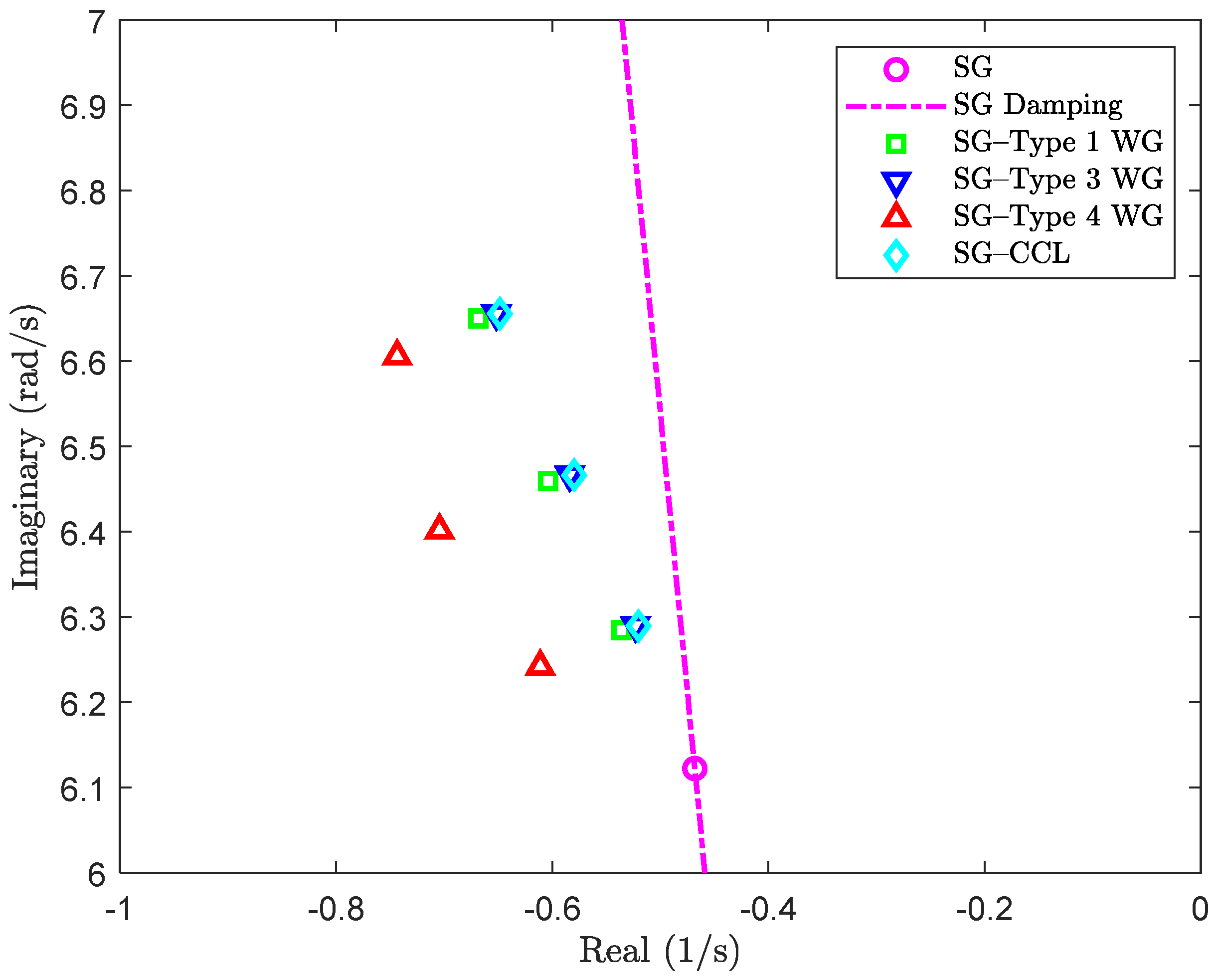
The impact of wind generation on the damping and frequency of power system electromechanical oscillation is evaluated by increasing the amount of wind generation while decreasing the amount of synchronous generation. Figure 11 displays the SG electromechanical eigenvalue shift as the proportion of wind generation increases. The damping of the electromechanical oscillation without wind generation is also displayed with a dash-dot line.

Figure 11 shows that the damping and the frequency of the SG electromechanical oscillation increase as the proportion of wind generation increases. This fact can be explained in terms of the lack of inertia of WGs: as WG increases, only SG inertia remains, resulting in higher electromechanical oscillation frequency and damping. The impact of the type 4 WF is higher than the impact of the types 1 and 3 WGs.

The impact of representing WGs as Constant Current Loads (CCLs) is also assessed. It should be noted that the electromechanical eigenvalues obtained representing the WG as a CCL are closed to the electromechanical eigenvalues when the WG is either type 1 or 3.

9. Conclusions

This paper has investigated the dynamic patterns in the small-signal behavior of power systems with wind power generation using very detailed models of wind generators, in contrast with the more simplified models used in electromechanical analysis and simulation of power systems. Close associations between eigenvalues and state variables of SGs and WGs have been identified using participation factors. It has been found that the dynamics of WGs are fairly decoupled from the dynamics of SGs. In other words, SGs and WGs exhibit distinct dynamic patterns. Hence simplified.

In addition, this paper has included a fundamental study on the effect of wind power generation on power system small-signal stability. Precisely, the effect of wind power generators of three different technologies (types 1, 3, and 4 WGs) on the damping and frequency of the electromechanical oscillation of a synchronous generator has been determined. A simple power system built of two generators (SG and WG) has been considered, and the wind generation was increased while the synchronous generation was reduced. The increase in wind generation results in an increase in the damping and frequency of the electromechanical oscillation. In addition, constant current load models can be used to represent types 1 and 3 for small-signal stability studies.

References

- Kundur, P. Power System Stability and Control; Mc Graw Hill: New York, NY, USA, 1994. [Google Scholar]
- Hatziargyriou, N.; Milanovic, J.; Rahmann, C.; Ajjarapu, V.; Canizares, C.; Erlich, I.; Hill, D.; Hiskens, I.; Kamwa, I.; Pal, B.; et al. Definition and Classification of Power System Stability—Revisited & Extended. IEEE Trans. Power Syst. 2021, 36, 3271–3281. [Google Scholar]
- Sanchez-Gasca, J.J.; Miller, N.W.; Price, W.W. A Modal Analysis of a Two-area System with Significant Wind Power Penetration. In Proceedings of the 2004 IEEE PES Power Systems Conference and Exposition, New York, NY, USA, 10–13 October 2004; Volume 2, pp. 1148–1152. [Google Scholar]
- Mendonca, A.; Lopes, J.A.P. Impact of Large-scale Wind Power Integration on Small-signal Stability. In Proceedings of the 2005 International Conference on Future Power Systems, Amsterdam, The Netherlands, 16–18 November 2005. [Google Scholar]
- Vowles, D.J.; Samarasinghe, C.; Gibbard, M.J.; Ancell, G. Effect of Wind Generation on Small-signal—A New Zealand Example. In Proceedings of the 2008 IEEE Power and Energy Society General Meeting, Pittsburgh, PA, USA, 20–24 July 2008. [Google Scholar]
- Gautam, D.; Vittal, V.; Harbour, T. Impact of Increased Penetration of DFIG-Based Wind Turbine Generators on Transient and Small Signal Stability of Power Systems. IEEE Trans. Power Syst. 2009, 24, 1426–1434. [Google Scholar] [CrossRef]
- Tsourakis, G.; Nomikos, B.M.; Vournas, C.D. Contribution of Doubly Fed Wind Generators to Oscillation Damping. IEEE Trans. Energy Convers. 2009, 24, 783–791. [Google Scholar] [CrossRef]
- Wilches-Bernal, F.; Lackner, C.; Chow, J.H.; Sanchez-Gasca, J.J. Small-signal Analysis of Power System Swing Modes as Affected by Wind Turbine-generators. In Proceedings of the 2016 IEEE Power and Energy Conference at Illinois, Urbana, IL, USA, 19–20 February 2016. [Google Scholar]
- Hughes, F.M.; Anaya-Lara, O.; Jenkins, N.; Strbac, G. A Power System Stabilizer for DFIG-based Wind Generation. IEEE Trans. Power Syst. 2006, 21, 763–772. [Google Scholar] [CrossRef]
- Sigrist, L.; Rouco, L. Design of Damping Controllers for Doubly Fed Induction Generators Using Eigenvalue Sensitivities. In Proceedings of the 2009 IEEE Power Systems Conference and Exposition, Seattle, WA, USA, 15–18 March 2009. [Google Scholar]
- Anaya-Lara, O.; Jenkins, N.; Ekanayake, J.; Cartwright, P.; Hughes, M. Wind Energy Generation; John Wiley and Sons: Hoboken, NJ, USA, 2009. [Google Scholar]
- Sørensen, P.; Andresen, B.; Fortmann, J.; Pourbeik, P. Modular structure of wind turbine models in IEC 61400-27-1. In Proceedings of the 2013 IEEE Power & Energy Society General Meeting, Vancouver, BC, Canada, 21–25 July 2013. [Google Scholar]
- Gomez-Exposito, A.; Conejo, A.J.; Cañizares, C. (Eds.) Electric Energy Systems: Analysis and Operation; CRC Press: Boca Raton, FL, USA, 2008. [Google Scholar]
- Pena, R.; Clare, J.C.; Asher, G.M. Doubly fed induction generator using back-to-back PWM converters and its application to wind-energy generation. IEE Proc. Electron. Power Appl. 1996, 143, 231–241. [Google Scholar] [CrossRef]
- Rouco, L.; Zamora, J.L. Dynamic Patterns and Model Order Reduction in Small-signal Models of Doubly Fed Induction Generators for Wind Power Applications. In Proceedings of the 2006 IEEE/PES General Meeting, Montreal, QC, Canada, 18–22 June 2006. Paper 06GM1126. [Google Scholar]
- Hünemörder, S.; Bierhoff, M.; Fuchs, F.W. Drive with Permanent Magnet Synchronous Machine and Voltage Source Inverter for Wind Power Application. In Proceedings of the NORPIE 2002, Nordic Workshop on Power and Industrial Electronics, Stockholm, Sweden, 12–14 August 2002. [Google Scholar]
- Achilles, S.; Pöller, M. Direct Dirve Synchronous Machine Models for Stability Assessment of Wind Farms. In Proceedings of the 4th International Workshop on Large Scale Integration of Wind Power and Transmission Networks for Offshore Wind-Farms, Billund, Denmark, 20–21 October 2003. [Google Scholar]
- Tabernero, J.; Rouco, L. Dynamic Patterns in Small-signal Models of Multipole Synchronous Generators for Wind Power Applications. In Proceedings of the IEEE Power Tech 2007, Lausanne, Switzerland, 1–5 July 2007. [Google Scholar]
- Pérez-Arriaga, I.J.; Verghese, G.C.; Schweppe, F.C. Selective Modal Analysis with Applications to Electric Power Systems. Part I: Heuristic Introduction. Part II: The Dynamic Stability Problem. IEEE Trans. Power Appar. Syst. 1982; PAS-101, 3117–3134. [Google Scholar]
- D’Arco, S.; Suul, J.A.; Fosso, O.B. Automatic Tuning of Cascaded Controllers for Power Converters Using Eigenvalue Parametric Sensitivities. IEEE Trans. Ind. Appl. 2015, 51, 1743–1753. [Google Scholar] [CrossRef]
- Rouco, L.; Pagola, F.L.; Verghese, G.C.; Pérez-Arriaga, I.J. Selective Modal Analysis. In Power System Coherency and Model Reduction; Chow, J.H., Ed.; Springer: Berlin/Heidelberg, Germany, 2013. [Google Scholar]
Figure 1.
Equivalent circuit of an induction machine.
Figure 2.
Control scheme of a type 3 WG.
Figure 3.
Control scheme of the MSC of a type 3 WG.
Figure 4.
Control scheme of the GSC of a type 3 WG.
Figure 5.
Equivalent circuit of a doubly fed induction machine, including the filter of the grid-side converter.
Figure 6.
Control scheme of a multipole synchronous generator.
Figure 7.
Controllers of the MSC of a type 4 wind generator.
Figure 8.
Equivalent circuit of a multipole synchronous generator.
Figure 9.
A single-line diagram of a single generator connected to an infinite bus.
Figure 10.
Single-line diagram of a SG and a WG connected to an infinite bus.
Figure 11.
Variation in the electromechanical eigenvalue when wind generation increases in the test system is shown in Figure 10.