Prediction of Biogas Production Volumes from Household Organic Waste Based on Machine Learning

Abstract

The article proposes to use machine learning as one of the areas of artificial intelligence to forecast the volume of biogas production from household organic waste. The use of five regression algorithms (Linear Regression, Ridge Regression, Lasso Regression, Random Forest Regression, and Gradient Boosting Regression) to create an effective model for forecasting the volume of biogas production from household organic waste is considered. Based on the comparison of these algorithms by MSE and MAE indicators, the quality of training and their accuracy during forecasting are evaluated. The proposed algorithm for creating a model for forecasting biogas production volumes from household organic waste involves the implementation of 10 main and 3 auxiliary steps. Their advantage is that they aid in the performance of component data analysis, which is carried out based on the method of reducing the dimensionality of the data set, increasing interpretability, and minimizing the risk of data loss. An analysis of 2433 data is was carried out, which characterizes the formation of biogas from food (FW) and yard waste (YW) according to four features. Data preparation is performed using the Jupyter Notebook environment in Python. We select five machine learning algorithms to substantiate an effective model for forecasting volumes of biogas production from household organic waste. On the basis of the conducted research, the main advantages and disadvantages of the used algorithms for building forecasting models of biogas production volumes from household organic waste are determined. It is found that two models, “Random Forest Regressor” and “Gradient Boosting Regressor”, show the best accuracy indicators. The other three models (Linear Regression, Ridge Regression, Lasso Regression) are inferior in accuracy and were not considered further. To determine the accuracy of the “Random Forest Regressor” and “Gradient Boosting Regressor” models, we choose the MSE and MAE indicators. The Random Forest Regressor model is found to be a more accurate model compared to the Gradient Boosting Regressor. This is confirmed by the fact that the MSE of the “Random Forest Regressor” model on the training data set is 7.14 times smaller than that of the “Gradient Boosting Regressor” model. At the same time, MAE is 2.67 times smaller in the “Random Forest Regressor” model than in the “Gradient Boosting Regressor” model. The MSE and MAE of both models are worse on the test data set, which indicates overtraining tendencies. The Gradient Boosting Regressor model has worse MSE and MAE than the Random Forest Regressor model on both the training and test data sets. It is established that the model based on the “Random Forest Regressor” algorithm is the most effective for forecasting the volume of biogas production from household organic waste. It provides MAE = 0.088 on test data and the smallest absolute errors in predictions. Further systematic improvement of the “Random Forest Regressor” model for forecasting biogas production volumes from household organic waste based on new data will ensure its accuracy and maintain competitive advantages.

1. Analysis of the State of the Art in Science and Justification of the Feasibility of Research

1.1. Introduction

Currently, processing waste into energy is an important step in the direction of creating sustainable energy in various countries of the world. This process makes it possible to reduce the volume of waste disposal, reduce dependence on fossil fuels, and create new jobs [1,2,3,4]. At the same time, household organic waste is a significant source of energy that can be used for biogas production. Anaerobic digestion of organic waste can potentially cover up to 1% of primary energy needs in the EU-27. At the same time, there is a significant potential for increasing the volume of organic waste for energy production from 4.7% to 71.2% of the total energy demand [5]. The potential of organic household waste as a source of energy depends on the region. More than 200 million tons of household waste are generated in Ukraine [6]. Biogas is a renewable source of energy that can be used for the production of electricity, thermal energy, and for activities in various industries. To increase the economic efficiency of biogas use, it is necessary to solve separate scientific and applied tasks. Ensuring the proper accuracy of solving such tasks requires the use of modern information technologies. In energy supply projects for consumers, which involve the use of organic waste for biogas production, one of the unresolved tasks is forecasting the volume of biogas production [7,8]. Accurate and fast implementation of the specified management process allows to assess the potential of biogas as an energy source and to determine the infrastructure needs for its production and use.

Machine learning is a powerful tool that researchers use to solve forecasting problems in various subject areas [9,10]. In our work, it is proposed to use machine learning as one of the directions of the functioning of artificial intelligence to forecast the volume of biogas production from organic household waste. The effectiveness of machine learning methods for forecasting the volume of biogas production depends on many factors, important of which are the quality of the collected and prepared data and the selected machine learning methods for creating an effective forecasting model.

Scientists have achieved significant success in the development and use of machine learning methods for forecasting in various areas of people’s lives and activities. However, the task of forecasting volumes of biogas production from household organic waste has been neglected. The novelty of the performed work is that, for the first time, a model based on the machine learning algorithm “Random Forest Regressor” is substantiated for forecasting the volume of biogas production from household organic waste. The obtained results are of practical value, since based on the obtained model, it is possible to develop a decision-making support system for forecasting the volume of biogas production from household organic waste.

1.2. Analysis of Published Data and Problem Sets

Forecasting the volume of biogas production from household organic waste is an important scientific and applied task, as it allows to assess the potential of biogas as an energy source and further determines the need for infrastructure for its production and use. In scientific works, individual authors conduct research on the justification of the toolkit and its use for forecasting the volume of biogas production [11,12,13,14]. Some of these works use traditional statistical methods such as regression analysis, while others use machine learning techniques.

The authors of well-known publications in the direction of creating forecasting models for various subject areas use separate approaches and tools for their implementation [15,16,17]. At the same time, traditional statistical methods, such as regression analysis, can be effective for forecasting biogas production volumes if the input data are well characterized [18,19]. However, these methods may not be accurate enough if the input data are complex or non-linear.

The methods based on computational intelligence, which are proposed to be used in works [20,21,22,23], are more accurate for forecasting the volumes of biogas production than traditional statistical methods. This is due to the fact that they provide training of models on historical data and offer detection of hidden patterns and their trends that cannot be detected visually. Some of the machine learning methods that are used to solve forecasting problems [24,25,26,27] deserve attention. They involve the use of machine learning methods to forecast biogas production volumes. Despite the availability of a number of scientific works devoted to forecasting the volume of biogas production, there are a number of shortcomings that must be resolved in order to increase the accuracy of forecasts [28,29,30]. One such drawback is that the input data for forecasting biogas production volumes may be incomplete or inaccurate. Also, the volume of biogas production is quite sensitive to the quality of raw materials. These factors should be taken into account when building predictive models based on machine learning.

Based on the analysis of scientific works, it was established that there is a need for the development and application of an effective model for forecasting the volume of biogas production from household organic waste. It should accurately and reliably forecast the volume of biogas production based on the known characteristics of household organic waste. The research results can be used to develop an intelligent information system for planning energy supply projects for consumers using organic waste.

The purpose of this article is to substantiate an effective model for forecasting the volume of biogas production from household organic waste based on the study of various machine learning methods. For this purpose, a real data set is used, which includes information about the state of organic waste that enters the biogas production, including its type, volume of solid organic substances, content of volatile organic substances, and biogas yield.

To achieve the goal, the following aims must be met:

–

development of an algorithm for determining an effective model for forecasting volumes of biogas production from household organic waste and to collect and prepare data;

–

justification an effective model for forecasting the volume of biogas production from organic household waste and to evaluate its accuracy.

Our article analyzes the state of science and practice in forecasting volumes of biogas production from waste. We collect and prepare the data, as well as select five regression algorithms for machine learning and substantiation of the model for forecasting the volume of biogas production from household organic waste. Based on the comparison of the obtained models by MSE and MAE indicators, the quality of training and model accuracies during forecasting are evaluated. This ensures the creation of an effective model for forecasting volumes of biogas production from household organic waste.

2. Development of an Algorithm for Determining an Effective Model for Forecasting Volumes of Biogas Production from Household Organic Waste and Data Collection and Preparation

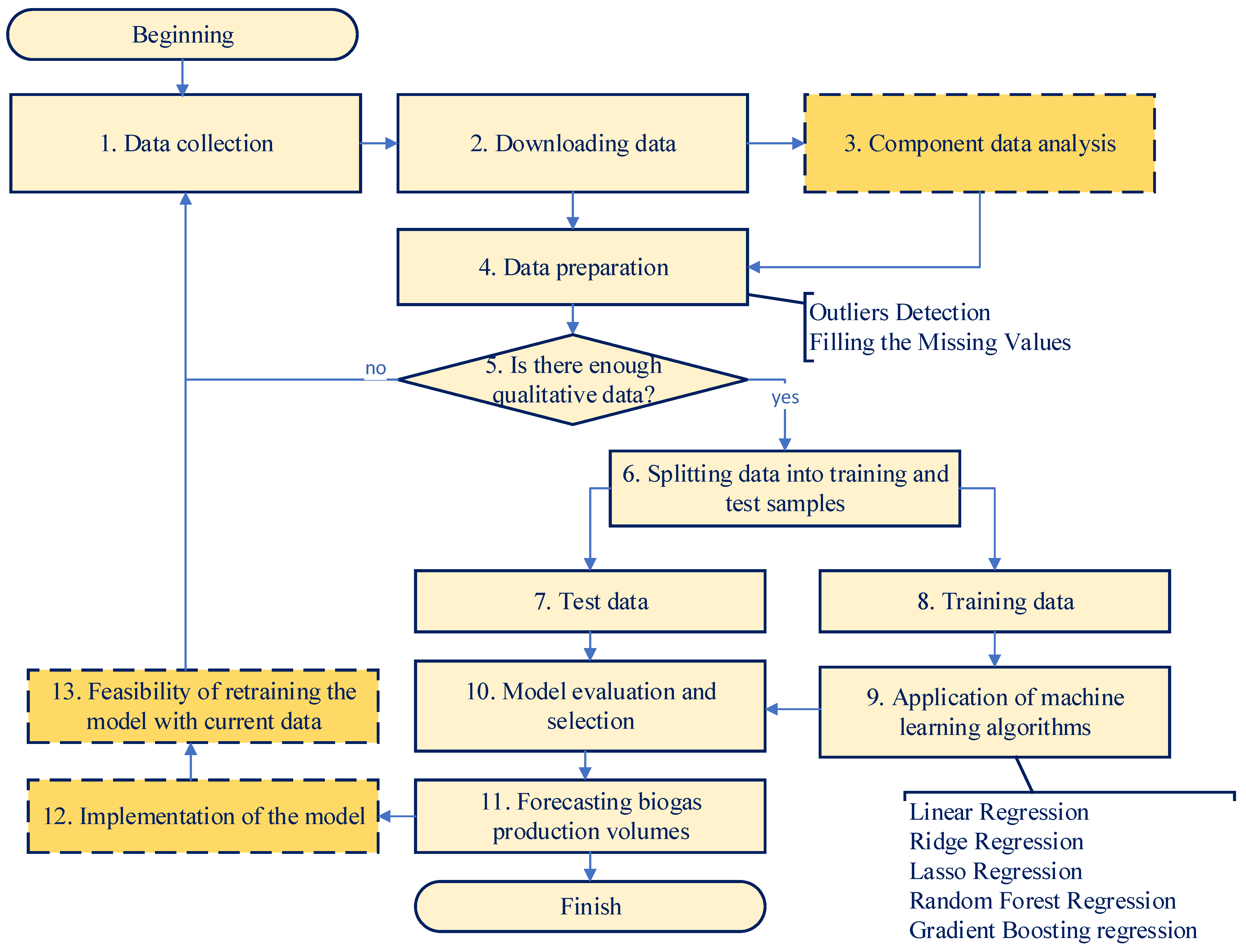
The creation of an effective model for forecasting the volume of biogas production from household organic waste is performed based on the algorithm presented in Figure 1. It envisages the use of machine learning methods to substantiate an effective model for forecasting the volume of biogas production from household organic waste based on the collected data. The aim is to build a model that provides accurate prediction of biogas yield (SGP) based on input data: type of waste (food FW or yard YW), total organic solids (TS), and volatile organics (TVS).

At the initial stage, the collection and preparation of the necessary data is carried out, which is the basis for the justification of an effective model for forecasting the volume of biogas production from organic household waste. At the same time, there are specific features that are reflected in the algorithm we develop (Figure 1). The target variable that we forecast is the amount of biogas output (SGP, m³/kg TVS) from organic household waste, which is determined by the following factors:

–

type of waste (FW and YW)—a categorical variable that determines the type of organic waste;

–

volume of solid organic substances (TS, kg/m³)—the amount of solid organic substances in organic waste;

–

by the content of volatile organic substances (TVS, % of TS)—the percentage of volatile organic substances from the total amount of solid organic substances.

The data upload process is performed in a CSV (Comma-Separated Values) format, which is quite standard and simple. Using CSV files is convenient for exchanging data between programs and for storing and processing data tables.

If necessary, the next step is component data analysis, which is performed based on the method of reducing the dimensionality of the data set, increasing interpretability, and minimizing the risk of data loss [31,32,33]. Thanks to this, a smaller number of sets of variables is created which belongs to the variables described above and, accordingly, contributes to the increase in variation in the data [34,35,36]. This analysis ensures the creation of linear combinations of the original observed variables that explain the largest variance in the data of a given component (Figure 2). Component analysis of the data is performed using the PCA package of the Scikit-learn library in the Python 3.11 programming language.

At the next stage, a description of the data preparation process is carried out, with the detection of gaps and the filling of missing values. Data preparation is an important process of any machine learning method [37,38,39,40,41,42]. It includes a number of tasks such as cleaning, standardizing, scaling, and sampling data. At the same time, one of the important tasks of data preparation is the identification and filling of gaps. Data gaps can occur for a variety of reasons, such as data entry errors, incomplete data sets, or failure to measure some values.

Data preparation is a key step in the machine learning process and involves several steps. Let us present a general overview of these steps. First of all, data collection is performed, as a result of which the desired data set $D$ is formed with the selection of input features and the outline $x_i$ of answers (labels) $y_i$:

$$D=\left\{\left(x_1,y_1\right),\left(x_2,y_2\right),\dots ,\left(x_n,y_n\right)\right\},$$

(1)

where $D$—data set; $x_i$—input characters, $y_i$—answers (marks).

The next step is to perform a data cleanup:

$$D_{clean}=f_{clean}\left(D\right),$$

(2)

where $D_{clean}$—cleaned data set.

After that, processing and filling of missing values is performed:

$$D_{imputed}=f_{impute}\left(D\right),$$

(3)

where $D_{imputed}$—a data set with recovered (filled) missing values.

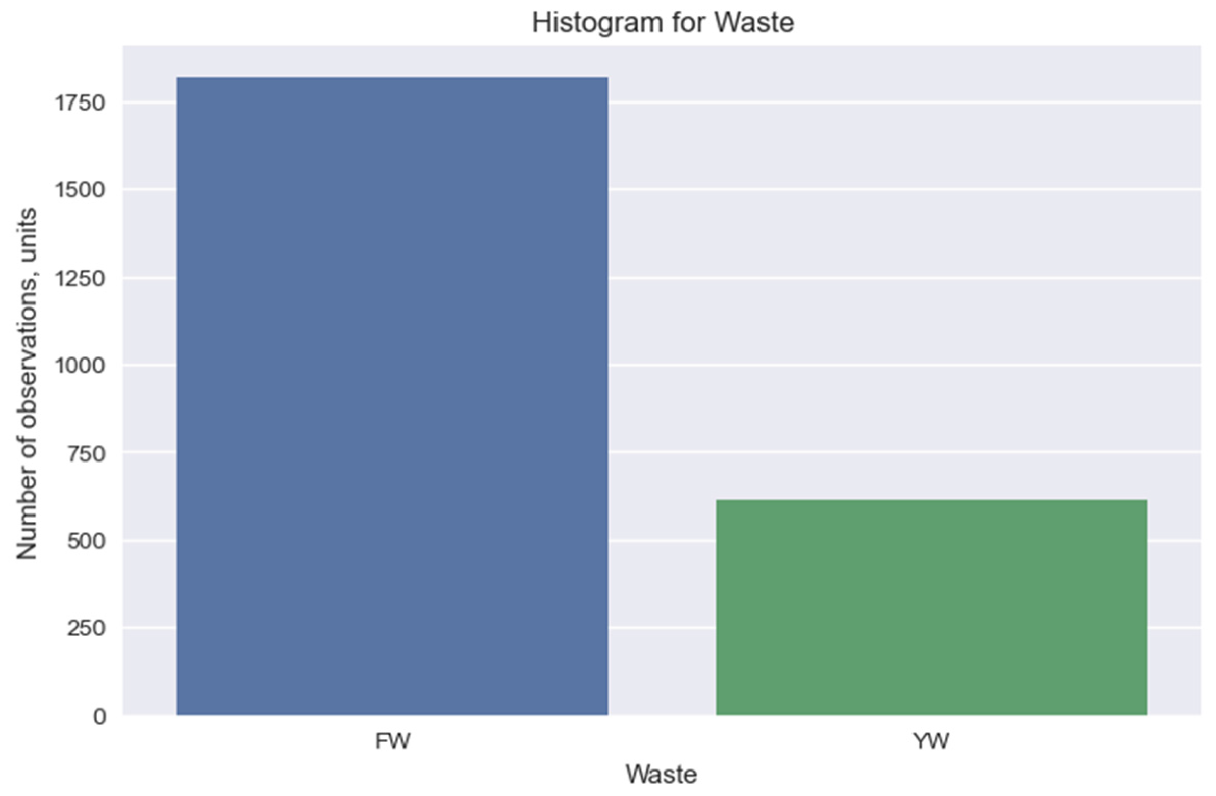
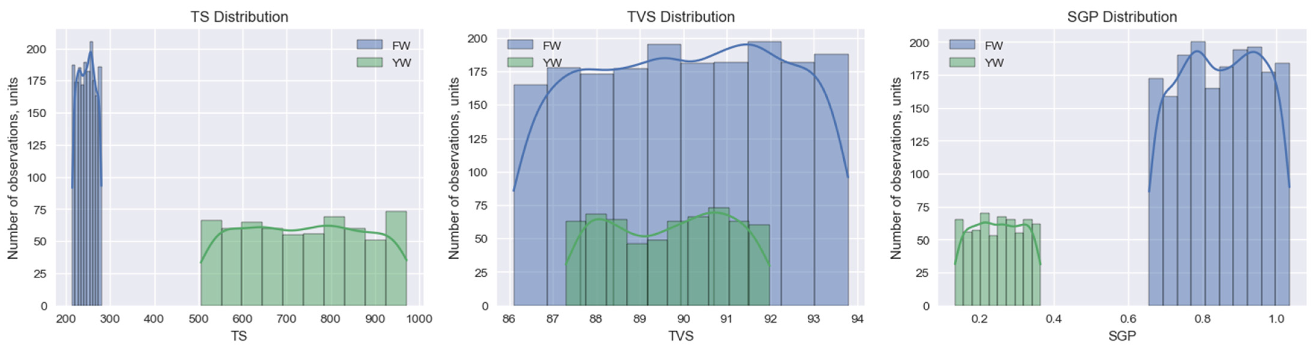
The Jupyter Notebook environment is used to prepare data on biogas production from household organic waste. This makes it possible to visualize the obtained results in a convenient format, which increases the efficiency of working with data despite performing separate data preparation operations. Based on the data analysis, we construct a histogram for two categories of waste (FW and YW) (Figure 3). Using the Matplotlib and Seaborn libraries, we plot the distributions of the volume of solid organic substances (TS, kg/m³), the content of volatile organic substances (TVS, % of TS), and the volume of biogas output (SGP, m³/kg TVS) (Figure 4).

The resulting histogram (Figure 3) indicates the distribution of categories in the “Waste” column. There are two unique data categories in our data set, which characterize food (FW) and yard waste (YW). At the same time, there are 1.818 instances of food (FW) and 615 of yard waste (YW) data.

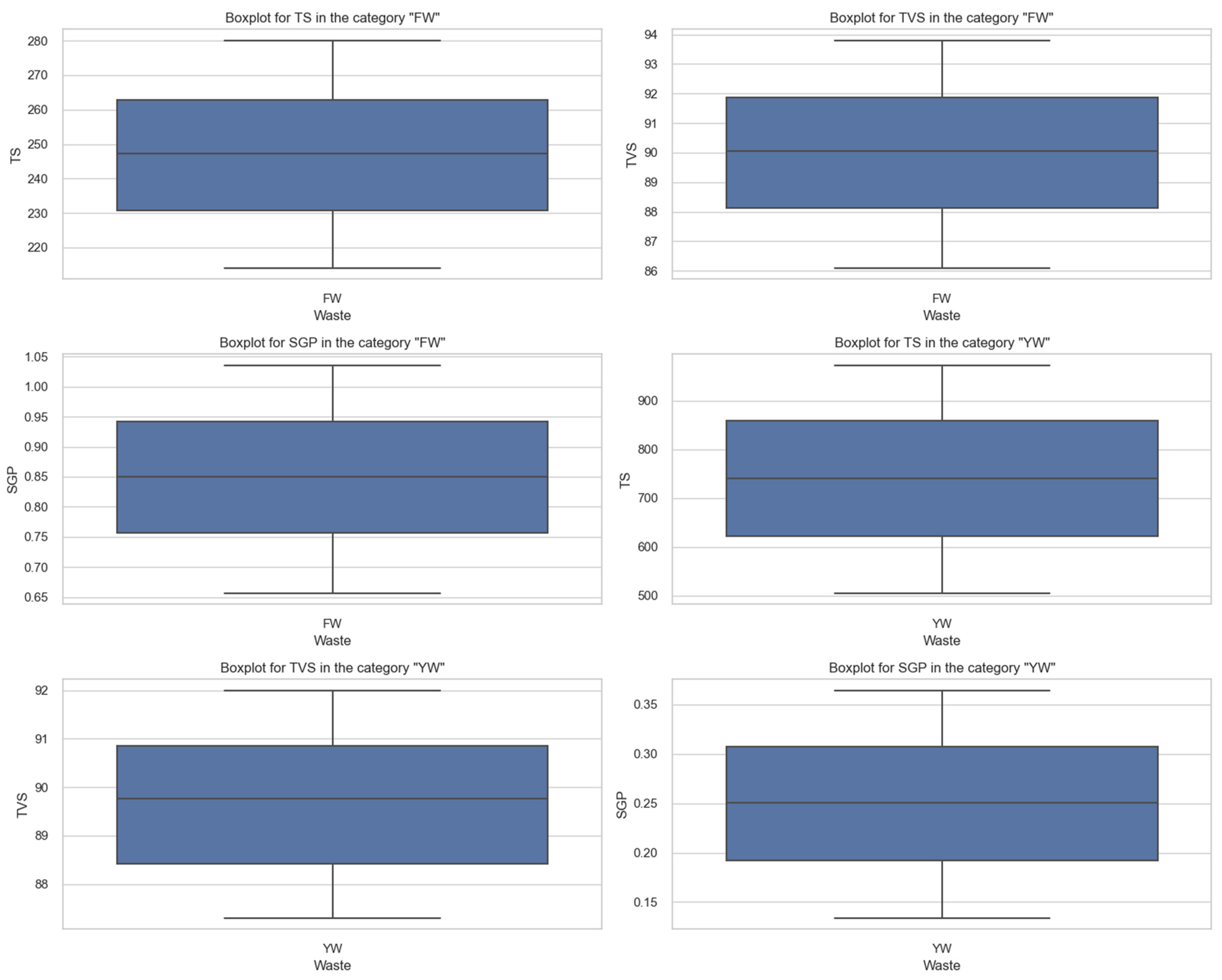
It is established that the characteristics of food (FW) and yard waste (YW) change in different ways, which requires their separate analysis. For this purpose, we construct diagrams of changes in the volume of solid organic substances (TS, kg/m³), the content of volatile organic substances (TVS, % of TS), and the volume of biogas output (SGP, m³/kg TVS) (Figure 5).

It is established that the amount of organic solids (TS) in FW food waste has an average value of TS of 247.0 kg/m³ and a small standard deviation of 18.9 kg/m³. At the same time, this indicator in YW yard waste has an average TS value of 738.6 kg/m³, and a much larger standard deviation of 138.0 kg/m³. Yard waste (YW) is found to have significantly higher mean and maximum TS compared to food waste (FW). This is due to a greater amount of wood, branches, and leaves in the yard mass.

Regarding the content of volatile organic substances (TVS), in FW food waste, the average value of TVS is 90.0%, the standard deviation is 2.2%. In YW yard waste, the average TVS value is 89.7%, and the standard deviation is 1.4%. The TVS content of both types of waste is found to be very similar. This indicates that they have a similar propensity for biodegradation.

Regarding the volume of biogas output (SGP), in FW, the mean value of SGP is 0.848 m³/kg TVS, and the standard deviation is 0.108 m³/kg TVS. Meanwhile, in YW yard waste, the mean value of SGP is 0.249 m³/kg TVS, and the standard deviation is 0.067 m³/kg TVS. It is found that FW has a significantly higher biogas generation potential compared to YW. This may be due to the higher concentration of easily decomposable organic substances in FW.

FW presents significantly higher biogas generation potential, making it more valuable. The obtained results indicate that the characteristics of FW and YW are significantly different. YW has higher TS and greater TS variability for anaerobic processing.

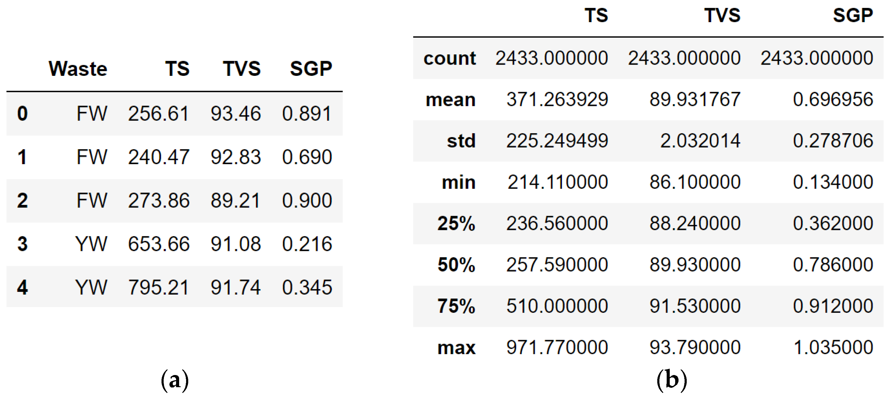
In order to perform a detailed analysis, we present the statistical characteristics of numerical variables regarding the volume of biogas production from household organic waste in

Table 1. Statistical characteristics of numerical variables regarding the volume of biogas production from household organic waste.

Type of Waste	Variable Value	Count	Mean	Std	Min	Distribution Quantiles			Max
						25%	50%	75%
FW	TS_FW	1818	247.0	18.9	214.1	230.8	247.1	262.7	279.9
YW	TS_YW	615	738.6	138.0	505.4	621.4	740.1	858.3	971.8
FW	TVS_FW	1818	90.0	2.2	86.1	88.1	90.1	91.9	93.8
YW	TVS_YW	615	89.7	1.4	87.3	88.4	89.8	90.8	91.9
FW	SGP_FW	1818	0.848	0.108	0.657	0.757	0.850	0.941	1.035
YW	SGP_YW	615	0.249	0.067	0.134	0.192	0.251	0.307	0.364

.

The amount of TS using FW has an average value (mean) of 247.0 kg/m³ and a standard deviation (std) of 18.9 kg/m³. The range of changes in the volume of solid organic substances (TS) ranges from 214.1 kg/m³ to 279.9 kg/m³. As for yard waste, the mean is 738.6 kg/m³, and the standard deviation (std) is 138.0 kg/m³. The range of changes in the volume of solid organic substances for this type of waste is from 505.4 kg/m³ to 971.8 kg/m³.

The content of volatile organic substances (TVS, % of TS) using FW has an average value (mean) of 90.0% and a standard deviation (std) of 2.2%. The range of changes in the content of volatile organic substances is from 86.1% to 93.8%. As for YW, the average value (mean) of the content of volatile organic substances is 89.7%, and the standard deviation (std) is 1.4%. The range of changes in the content of volatile organic substances for this type of waste is from 87.3% to 91.9%.

The amount of biogas output (SGP, m³/kg TVS) using FW has an average value (mean) of 0.848 m³/kg TVS and a standard deviation (std) of 0.108 m³/kg TVS. The range of changes in the volume of biogas output (SGP) is from 0.657 m³/kg TVS to 1.035 m³/kg TVS. Regarding YW, the average value (mean) of the volume of biogas output is 0.249 m³/kg TVS, and the standard deviation (std) is 0.067 m³/kg TVS. The amount of biogas output for this type of waste ranges from 0.134 m³/kg TVS to 0.364 m³/kg TVS.

The obtained statistical characteristics make it possible to gain an understanding of the distribution and features of each variable for both considered types of waste which affect the projected amount of biogas production from organic household waste.

In the next step, normalization and standardization of individual data features is performed, described by the following formulas [32]:

$$x_{normalized}=\frac{x-min\left(x\right)}{max\left(x\right)-min\left(x\right)},$$

(4)

where $x_{normalized}$—normalized value of the indicator; $x$—empirical value of the indicator; $min\left(x\right)$—smallest value of the indicator in the sample; $min\left(x\right)$—largest value of the indicator in the sample.

$$\begin{array}{l}\\ x_{standardized}=\frac{x-mean\left(x\right)}{std\left(x\right)}\end{array},$$

(5)

where $x_{standardized}$—standardized value of the indicator; $mean\left(x\right)$—average value of the indicator value in the sample; $std\left(x\right)$—standard deviation of the indicator in the sample.

After that, the coding of categorical features is performed [32]:

$$\begin{array}{l}\\ x_{encoded}=f_{encode}\left(x\right)\end{array},$$

(6)

where $x_{encoded}$—coded value of categorical features.

In our research, data preprocessing is performed using the Scikit-learn library in the Python programming language. This makes it possible to prepare data for forecasting the volume of biogas production from household organic waste, a fragment of which is shown in

Table 2. A fragment of prepared data for forecasting the volume of biogas production from household organic waste.

Observation	Waste	TS	TVS	SGP
–	X1	X2	X3	Y1
0	0	256.61	93.46	0.891
1	0	240.47	92.83	0.690
2	0	273.86	89.21	0.900
3	1	653.66	91.08	0.216
4	1	795.21	91.74	0.345
…	…	…	…	…
2430	0	243.11	88.18	1.010
2431	0	227.85	92.71	0.777
2432	0	231.58	89.56	0.795

.

In the next step, features are selected:

$$\begin{array}{l}\\ D_{selected}=f_{select}\left(D\right)\end{array},$$

(7)

where $D_{selected}$—data set with selected features.

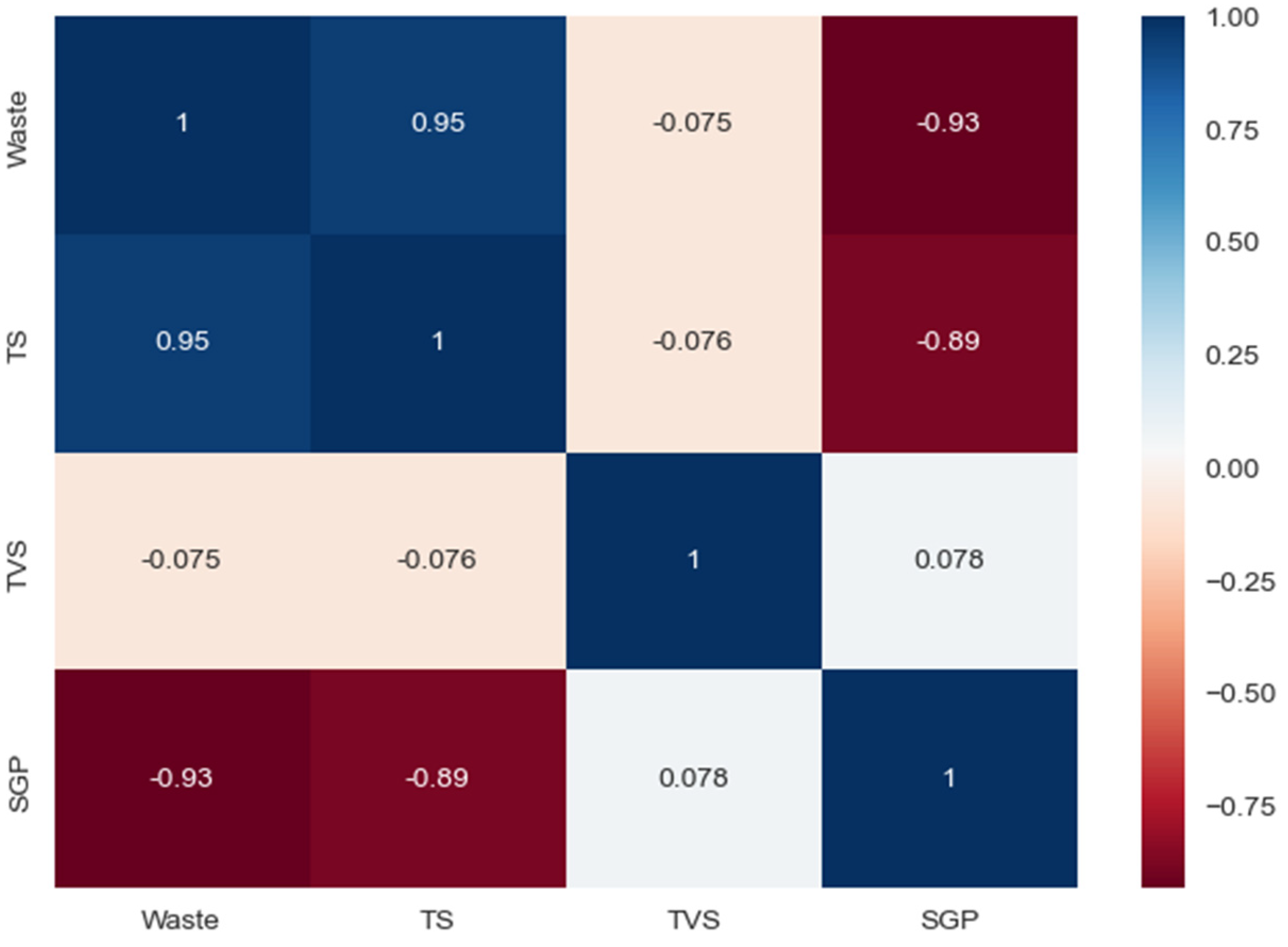
After that, the input parameters of the forecasting model of biogas production volumes from household organic waste are determined. We select the attributes that have the highest correlation with the target attribute “SGP”. For this, a correlation matrix is used (Figure 6). For each input parameter, their average value is determined (according to Table 2):

$${\overline{x}}_i=\frac{1}{n}{\displaystyle \sum _{i=1}^n{x}_{ij},j=1,m},$$

(8)

where ${\overline{x}}_i$—average value of the input parameter; $x_{ij}$—current value of the parameter; $n$—number of data instances; $m$—number of data attributes.

Quantitative values of the components of correlation matrix $k_{ij}$ are determined by formula [27]

$${\mathrm{k}}_{\mathrm{i}\mathrm{j}}=\frac{\mathrm{co}\mathrm{r}\mathrm{r}\left({\mathrm{x}}_{\mathrm{i}\mathrm{j}},{\mathrm{y}}_1\right)}{\sigma \left({\mathrm{x}}_{\mathrm{i}\mathrm{j}}\right),\sigma \left({\mathrm{y}}_1\right)},$$

(9)

where $\mathrm{co}rr\left(x_{ij},y_1\right)$—correlation between the input data and target feature $y_1$.

The correlation between the quantitative values of the input factors (x₁, …, x₃) and the target characteristic “SGP” ($y_1$) is determined by formula [27]

$$\mathrm{co}\mathrm{r}\mathrm{r}\left({\mathrm{x}}_{\mathrm{i}\mathrm{j}},{\mathrm{y}}_1\right)=\frac{{\displaystyle \sum _{\mathrm{l}=1}^{\mathrm{n}}\left({\mathrm{x}}_{\mathrm{l}\mathrm{i}}-{\overline{\mathrm{x}}}_{\mathrm{i}}\right)\left({\mathrm{x}}_{\mathrm{l}\mathrm{j}}-{\overline{\mathrm{x}}}_{\mathrm{j}}\right),\mathrm{i},\mathrm{j}=1,\mathrm{n}}}{\mathrm{n}-1}.$$

(10)

The correlation matrix (Figure 6) represents the relationships between the input attributes and the target feature in the data set $\left(D\right)$. For the target trait “SGP”, the correlation with other traits is determined by Formula (10).

The obtained results of the calculations regarding the determination of the quantitative values of the correlation coefficients are presented in

Table 3. The results of determining the correlation coefficients between the input attributes and the target feature “SGP”.

Attribute	Correlation Coefficient
Waste	−0.934
TS	−0.887
TVS	0.078

.

Based on the obtained values of the correlation coefficients between the input attributes and the target feature “SGP”, it should be noted that the attributes “Waste” and “TS” have a strong correlation with the attribute “SGP”, and the attribute “TVS” has a correspondingly weak correlation with the vector of target values (output variable).

In the future, the data are divided into training and test samples:

$$D_{train},D_{test}=f_{split}\left(D\right).$$

(11)

We suggest using 20% of the data for testing and the rest for training. That is, the ratio between training and test samples is $D_{train}:D_{test}=80:20$.

This helps assess the ability of the model to generalize knowledge on new, previously unseen data. We describe a general approach to preparing data for machine learning in order to forecast volumes of biogas production from household organic waste.

3. Results of the Substantiation of an Effective Model for Forecasting Volumes of Biogas Production from Household Organic Waste and to Evaluate Its Accuracy Indicators

In order to train the forecasting model of biogas production volumes from household organic waste, we selected the following algorithms: (1) Linear Regression; (2) Ridge Regression; (3) Lasso Regression; (4) Random Forest Regression; (5) Gradient Boosting Regression. Let us briefly describe each of these algorithms and their basic concept.

Widely used in the practice of machine learning when solving forecasting problems is Linear Regression, which is described by the following formula:

$$y={\beta }_0+{\beta }_1{x}_1+{\beta }_2{x}_2+\dots +{\beta }_n{x}_n+\epsilon$$

(12)

where $y$—target variable (biogas production); $x_1,x_2,\dots ,x_n$—signs (properties of organic waste); ${\beta }_0$—intercept; ${\beta }_1,{\beta }_2,\dots ,{\beta }_n$—regression coefficients; $\epsilon$—an error.

The following Ridge Regression is an adaptation of the popular and widely used Linear Regression algorithm. It improves upon conventional Linear Regression by slightly modifying its cost function, which is described by the following formula:

$$Loss={\displaystyle \sum _{i=1}^n{\left(y_i-\left({\beta }_0+{\beta }_1{x}_{i1}+{\beta }_2{x}_{i2}+\dots +{\beta }_n{x}_{in}\right)\right)}^2+\alpha {\displaystyle \sum _{j=1}^n{\beta }_j^2}},$$

(13)

where α—parameter of regularization.

The specified Equation (13) adds a regularization term containing squared coefficients (${\beta }_j^2$).

The Lasso Regression algorithm, widely used for solving forecasting problems, deserves attention:

$$Loss={\displaystyle \sum _{i=1}^n{\left(y_i-\left({\beta }_0+{\beta }_1{x}_{i1}+{\beta }_2{x}_{i2}+\dots +{\beta }_n{x}_{in}\right)\right)}^2+\alpha {\displaystyle \sum _{j=1}^n\left|{\beta }_j\right|}}.$$

(14)

Equation (14) adds a regularization term containing the absolute values of the coefficients (${\beta }_j$).

Random forest for regression is considered a very powerful and robust machine learning algorithm because it handles multivariate data, missing values, and outliers well. Random Forest Regression (Random Forest for regression) involves a combination of many decision trees (Random Forest trees). We mark ${\widehat{y}}_i$ as a prediction from the ith tree; then,

$$\widehat{y}=\frac{1}{N}{\displaystyle \sum _{i=1}^N{\widehat{y}}_i},$$

(15)

where $\widehat{y}$—as a prediction from i tree; $N$—the number of trees in the ensemble.

Each tree offers, from Expression (15), its prediction, and as a result, the Random Forest averages or votes for these predictions. At the same time, the Random Forest reduces overtraining and ensures the importance of features.

Gradient Boosting Regression involves using a combination of weak models (usually decision trees). Each new model corrects the mistakes of the previous model. The forecast is formed as a weighted sum of the forecasts of all with the number of models $f_1,f_2,\dots ,f_M$, with the number of models $\left(M\right)$:

$$\widehat{y}=f_1\left(x\right)+f_2\left(x\right)+\dots +f_M\left(x\right).$$

(16)

Each model is added with a weight, depending on the learning rate:

$$\widehat{y}={\displaystyle \sum _{m=1}^M{\gamma }_m{f}_m\left(x\right)}.$$

(17)

where $\widehat{y}$—prediction from i of the model; $N$—number of models in the ensemble; ${\gamma }_m$—the weight m—the model has in gradient boosting.

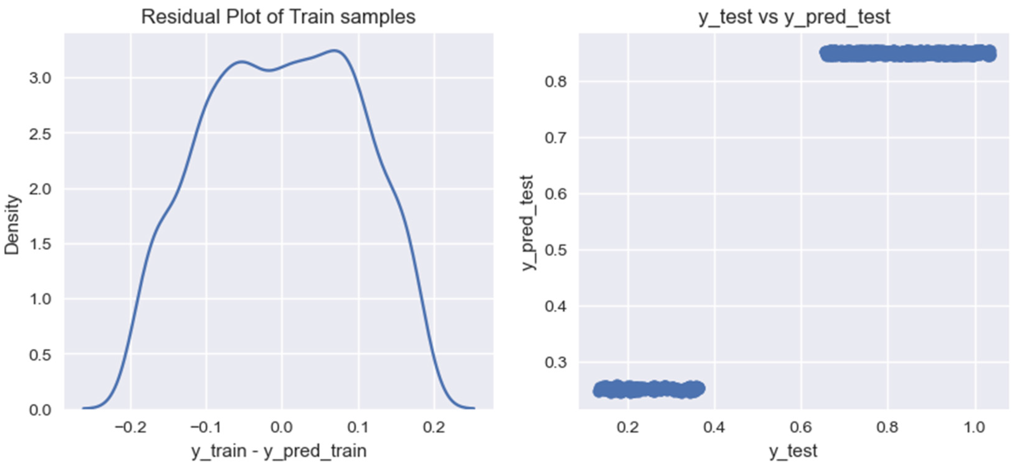
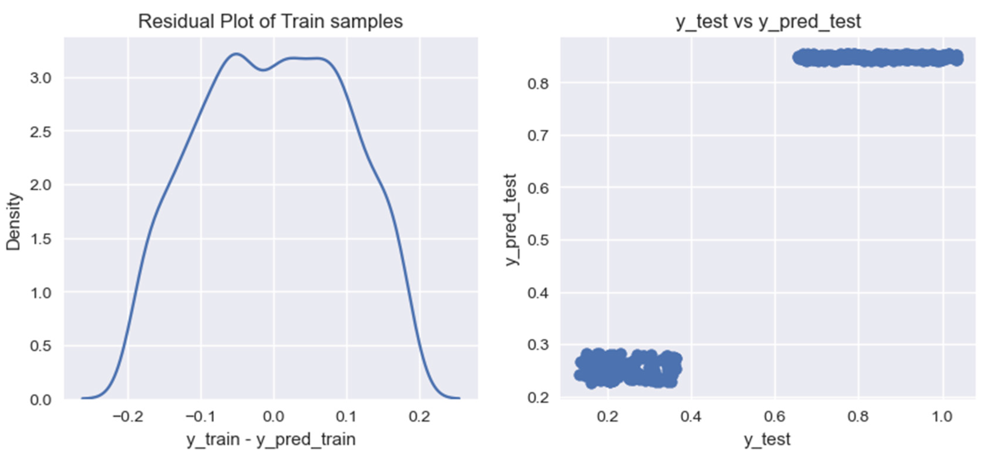
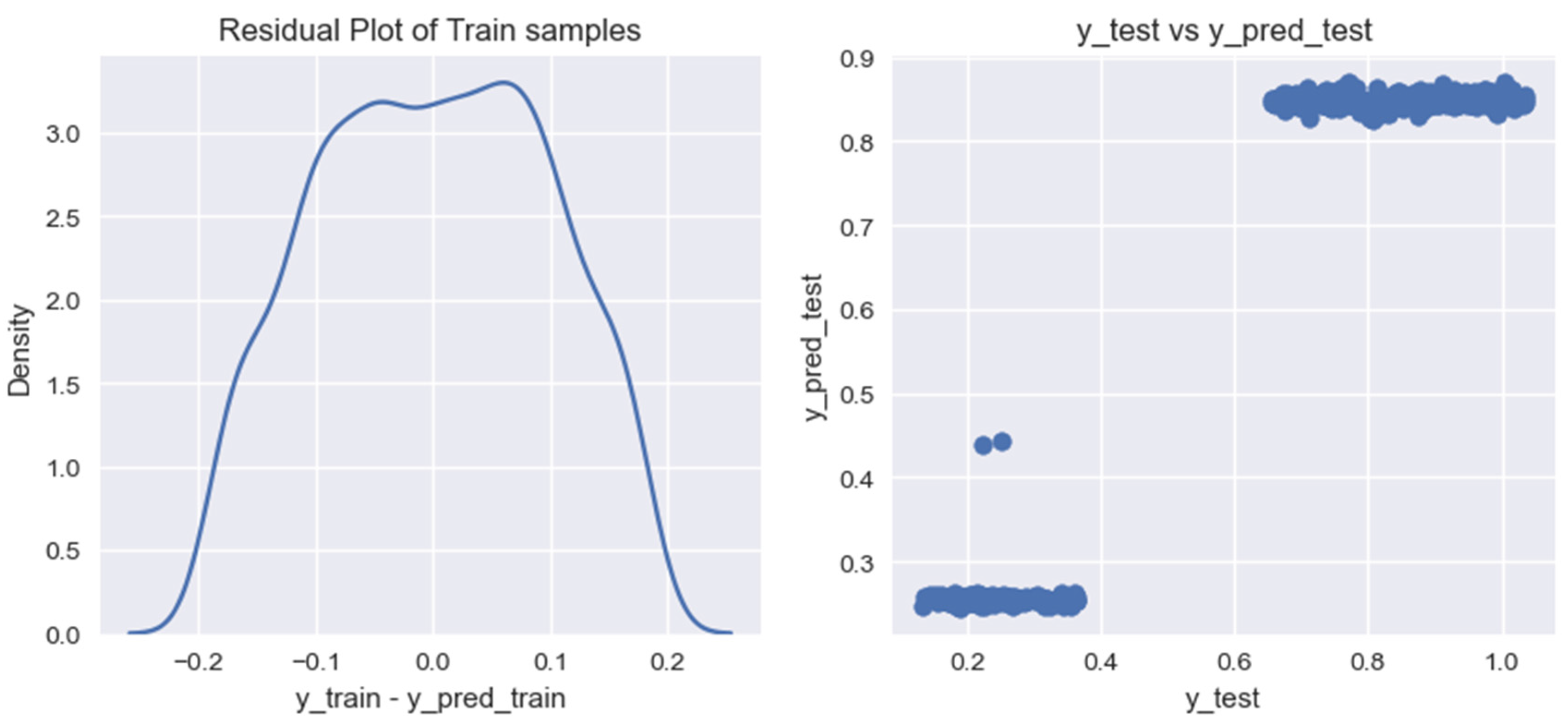
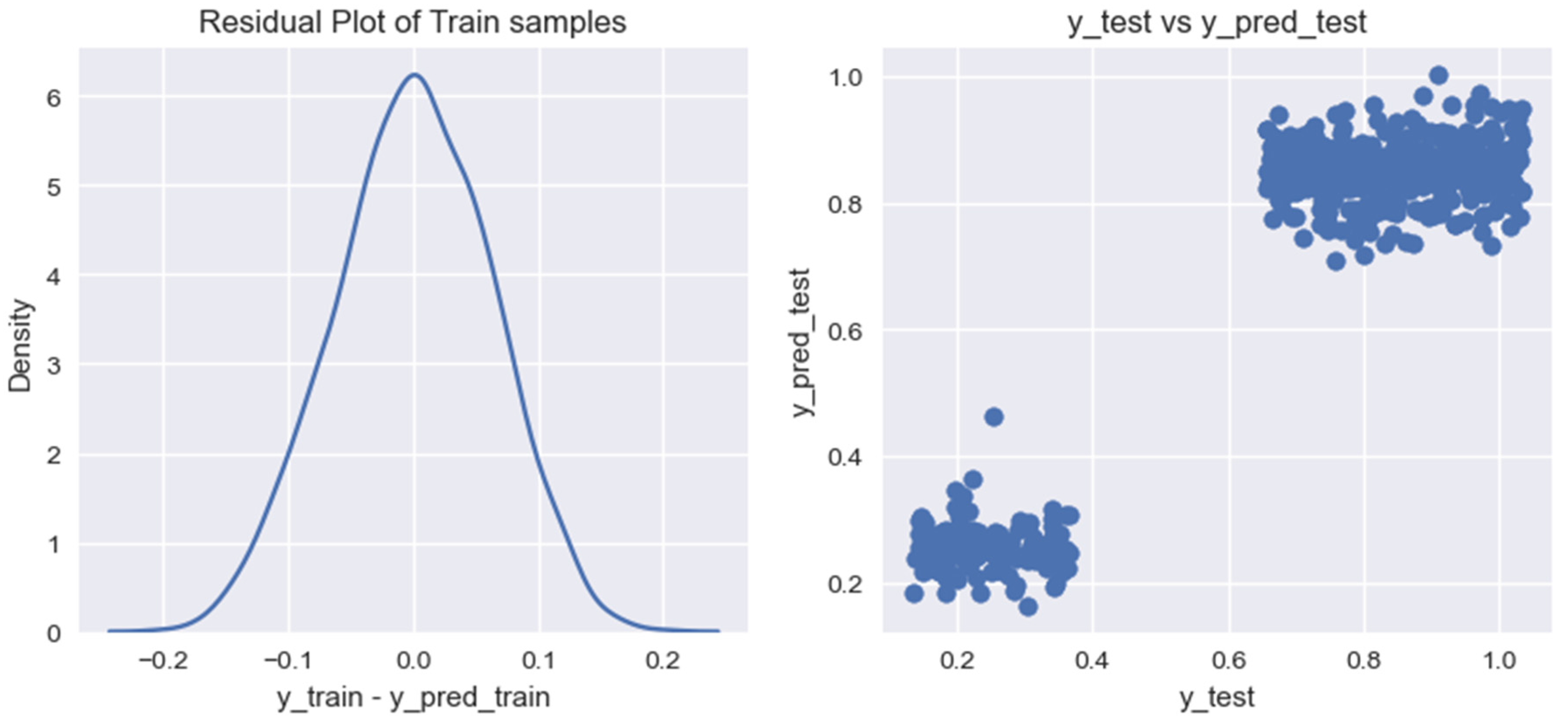
We use the specified algorithms to train a model for forecasting the volume of biogas production from household organic waste. As a result of our research, for each of the created models, we built graphs for residual analysis (residual) on training data (Figure 7, Figure 8, Figure 9, Figure 10 and Figure 11).

Based on the graphs of the residual values on the training data for the researched models of forecasting the volumes of biogas production from organic household waste, it can be noted that the models provide different results in terms of their accuracy. For a more accurate assessment of the obtained models, we calculated the following indicators: (1) coefficient of determination for the training data set, $R_{train}^2$; (2) coefficient of determination for the test data set, $R_{test}^2$; (3) mean cross-validation score for the training data set, $CV score mea{n}_{train}$.

The coefficient of determination ($R_{train}^2$) for the training data set indicates the percentage of variation of the dependent variable:

$$R_{train}^2=1-\frac{{\displaystyle \sum _{i=1}^n{\left(y_i-\widehat{y}\right)}^2}}{{\displaystyle \sum _{i=1}^n{\left(y_i-\overline{y}\right)}^2}},$$

(18)

where $n$—number of observations; $y_i$—real values of the target variable “SGP”; $\widehat{y}$—predicted values of “SGP” are derived from the model; $\overline{y}$—mean value of target variable “SGP”.

The coefficient of determination ($R_{test}^2$) for the test data set indicates how effectively the model matches the test data, i.e., evaluates the model’s fit with new, previously unseen data:

$$R_{test}^2=1-\frac{{\displaystyle \sum _{i=1}^n{\left(y_i-\widehat{y}\right)}^2}}{{\displaystyle \sum _{i=1}^n{\left(y_i-\overline{y}\right)}^2}}.$$

(19)

The average cross-validation score for the training data set $CV score mea{n}_{train}$ provides an estimate of the model’s performance based on cross-validation, taking into account the average value of the accuracy scores on different subsamples:

$$CV score mea{n}_{train}=\frac{1}{K}{\displaystyle \sum _{k=1}^K{R}_{train,k}^2}.$$

(20)

where $K$—the number of convolutions in cross-validation; $R_{train,k}^2$—coefficient of determination of the training data set $R_{train}^2$ for each convolution $k$.

This means that indicator $CV score mea{n}_{train}$ helps to evaluate the model’s resistance to variability in the training set using cross-validation.

The obtained results of the calculations regarding the model training accuracy indicators are presented in

Table 4. The results of determining the accuracy indicators of model training for forecasting the volumes of biogas production from organic household waste.

No.	Model	R2 (Train)	R2 (Test)	CV Score Mean (Train)
1	Linear Regression	0.87	0.87	0.87
2	Ridge Regression	0.87	0.87	0.87
3	Lasso Regression	0.87	0.87	0.87
4	Random Forest Regressor	0.88	0.87	0.87
5	Gradient Boosting Regressor	0.95	0.85	0.85

.

Considering the obtained results, it should be noted that the “Gradient Boosting Regressor” model provides the highest coefficient of determination, $R_{train}^2=0.95$, on the training data, which indicates the good ability of the model to explain the variation in the training data. However, on test data, this indicator is smaller and amounts to $R_{test}^2=0.85$, which indicates retraining of the model on training data and incomplete generalization on new data. At the same time, the “Random Forest Regressor” model provides the highest coefficient of determination, $R_{train}^2=0.88$, on the training data, and on the test data this indicator is somewhat smaller and is $R_{test}^2=0.87$, which indicates retraining of the model on training data and incomplete generalization on new data. As for the root mean square error, all the studied models have the same indicator, $CV score mea{n}_{train}=0.87$, on the training data.

However, the assessment of which model is best for predicting biogas production from household organic waste depending on the specific requirements and context of the problem regarding its accuracy. At the same time, one should take into account the interpretability of the model for forecasting volumes of biogas production from household organic waste and the speed of its learning.

To determine the accuracy of “Random Forest Regressor” and “Gradient Boosting Regressor” models, we chose MSE and MAE indicators. They provide an assessment of the accuracy of the specified model during its training and testing. They provide an evaluation of the model’s performance during different training epochs. The definition of MSE (mean squared error) involves the calculation of the root mean square difference between the predicted values of biogas production volumes from household organic waste using the model and the real biogas production values:

$$\mathrm{MSE}=\frac{1}{n}{\displaystyle \sum _{i=1}^n{\left(y_i-{\widehat{y}}_i\right)}^2}.$$

(21)

where $y_i$—value of biogas production volume from household organic waste, m³/kg TVS; ${\widehat{y}}_i$—forecast value of biogas production volume from household organic waste, m³/kg TVS; $n$—number of examples in the initial data array, units.

The next indicator that characterizes the accuracy of the model is the MAE (mean absolute error), which characterizes the average value of the difference between the predicted values of the model and the real values of the volume of biogas production from household organic waste:

$$\mathrm{MAE}=\frac{1}{n}{\displaystyle \sum _{i=1}^n\left|y_i-{\widehat{y}}_i\right|}.$$

(22)

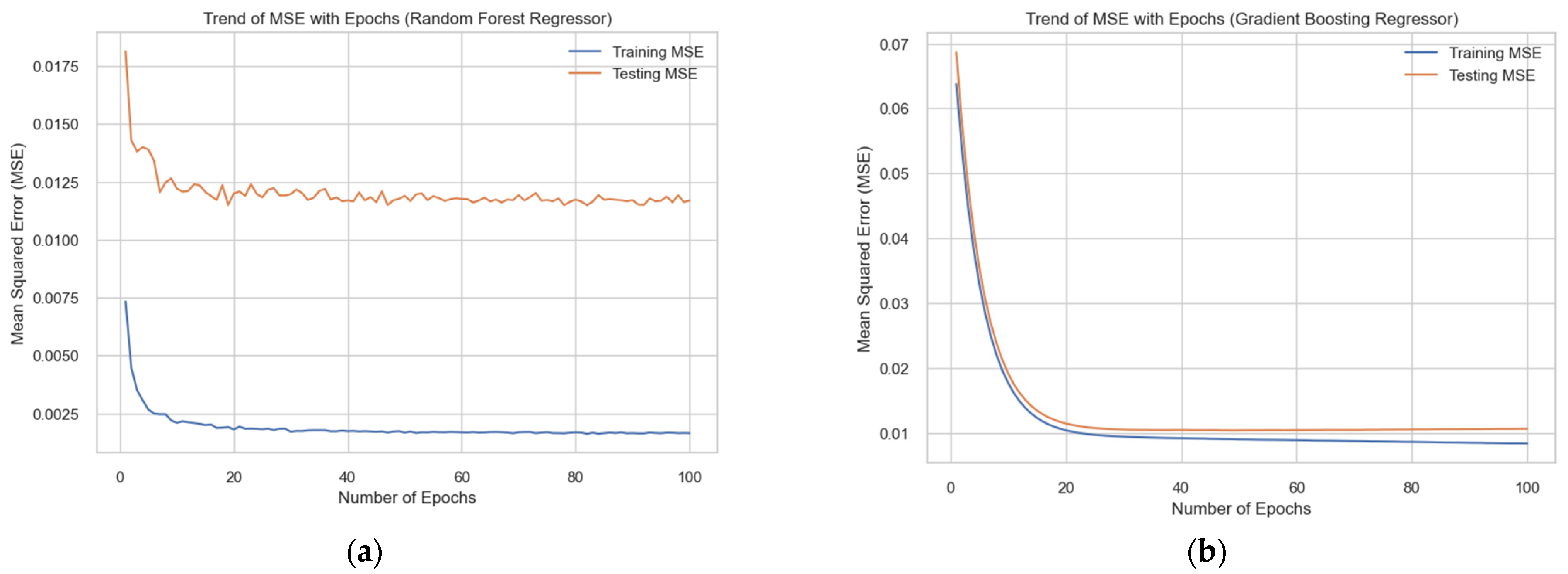
On the basis of the conducted research, we constructed the dependence of the change in the MSE indicator on the number of learning epochs using the “Random Forest Regressor” and “Gradient Boosting Regressor” models to forecast the volume of biogas production from household organic waste (Figure 12).

The obtained dependences of the change in the MSE indicator on the number of training epochs for the training and test data samples using the “Random Forest Regressor” and “Gradient Boosting Regressor” models indicate slightly different trends in the change in the indicated indicator. In particular, in the “Random Forest Regressor” model, a higher and unstable value of the indicated indicator is observed. At the same time, in the “Gradient Boosting Regressor” model, after 40 training epochs, the MSE indicator on the test sample increases compared to the training sample, which indicates that the model is retrained. We perform an analysis of the quantitative values of MSE and MAE indicators when forecasting the volume of biogas production from household organic waste using the studied models according to the data in

Table 5. Quantitative values of MSE and MAE indicators when forecasting biogas production volumes from household organic waste using the studied models.

No.	Model	MSE (Training)	MSE (Testing)	MAE (Training)	MAE (Testing)
1	Random Forest Regressor	0.001637	0.011698	0.033248	0.088905
2	Gradient Boosting Regressor	0.008365	0.010619	0.077221	0.087593

.

Based on the obtained data in Table 5, it was established that for the training sample, the “Random Forest Regressor” model has a smaller value of MSE = 0.001637, which indicates a good fit for the training data. For the test sample, the “Random Forest Regressor” model also has the smallest value of MSE = 0.011698, which confirms the effectiveness of the model on new data. At the same time, both models show low MSE values, but the “Random Forest Regressor” model looks more efficient for the test sample.

For the training sample, the “Random Forest Regressor” model also has the smallest value of MAE = 0.033248, which indicates accurate prediction on the training data. For the test sample, the “Random Forest Regressor” model has the smallest value of MAE = 0.088905, which is low and shows the effectiveness of the model on new data. In both cases, the Random Forest Regressor model has a smaller MAE value, indicating better accuracy compared to the Gradient Boosting Regressor model. Overall, the Random Forest Regressor model shows better performance for both metrics on the test sample compared to the Gradient Boosting Regressor model.

On the basis of the developed models, a graph of the actual and predicted values of biogas production from household organic waste was plotted using the “Random Forest Regressor” and “Gradient Boosting Regressor” models (Figure 13).

The resulting graph (Figure 13) shows how the developed models predict the actual values of the volume of biogas production from household organic waste. The observed actual values and the predicted values are close to each other, which means that the proposed model does a good job of forecasting. Based on the conducted research, it can be stated that the “Random Forest Regressor” model is the most effective for forecasting the volume of biogas production from household organic waste. This is confirmed by the fact that it has a smaller MAE value on the test data, which indicates smaller absolute errors in the predictions.

4. Discussion of Research Results

The obtained research results made it possible to justify the “Random Forest Regressor” model for forecasting the volume of biogas production from household organic waste based on machine learning. It will be useful in practice for information technology professionals and project managers who develop decision support systems for organic waste management and justify energy production strategies from this waste. The proposed model analyzes the input data which include the type of waste (FW and YW), the amount of solid organic matter (TS, kg/m³), and the content of volatile organic matter (TVS, % of TS) which affect the amount of biogas output (SGP, m³/kg TVS) from household organic waste. Through a balanced analysis of these factors, the model provides forecasts of biogas yield (SGP, m³/kg TVS) from household organic waste with high accuracy, helping to optimize the use of resources and increase production efficiency.

We selected five machine learning algorithms to substantiate an effective model for forecasting volumes of biogas production from household organic waste. On the basis of the performed research, the main advantages and disadvantages of the used algorithms were determined. The advantage of the “Linear Regression” algorithm is the ease of interpretation. In particular, Linear Regression is easily interpreted, which allows understanding of the effect of each characteristic on the target variable. Also, this algorithm provides adequate learning speed, and it has wide application in various fields. Its main drawback is that the resulting model assumes a linear relationship between the features and the target variable, which may not be sufficient for complex data. Also, it has an increased tendency to overtraining if there is a large number of correlational signs. The “Ridge Regression” algorithm involves the introduction of an additional term to the model loss function in order to limit the values of the model parameters. This helps to avoid overtraining. It has stability as it works well with multi-collinearity. The main disadvantage of the specified algorithm is the need to adjust the parameters. That is, it requires selection of the regularization parameter.

The “Lasso Regression” algorithm has an advantage over the other mentioned algorithms, as it provides automatic feature selection. At the same time, regularization can automatically select important features, which helps to avoid retraining and makes it possible to obtain a general model. Its main drawback is that there is a need to determine the optimal value of the regularization parameter, which will ensure better overall model efficiency.

The “Random Forest Regressor” algorithm provides high accuracy and is well suited for complex data with a large number of features. It is less prone to overtraining compared to some other algorithms. Its main drawback is the difficulty of interpretation. That is, a more complex process of interpretation is inherent compared to linear models.

The “Gradient Boosting Regressor” algorithm provides high accuracy, especially on data sets with a large number of features. It is suitable for the automatic selection of important features. The disadvantage is that this algorithm is prone to overtraining. Overlearning may occur with insufficiently configured hyperparameters. In addition, it requires fine-tuning of hyperparameters to achieve optimal performance.

Based on the conducted research, it was established that two models, “Random Forest Regressor” and “Gradient Boosting Regressor”, show the best accuracy indicators. The other three models (Linear Regression, Ridge Regression, Lasso Regression) are inferior in accuracy and were not considered further. To determine the accuracy of “Random Forest Regressor” and “Gradient Boosting Regressor” models, we chose MSE and MAE indicators. The Random Forest Regressor model was found to be a more accurate model compared to the Gradient Boosting Regressor. This is confirmed by the fact that the MSE of the “Random Forest Regressor” model on the training data set is 7.14 times smaller than that of the “Gradient Boosting Regressor” model. At the same time, MAE is 2.67 times smaller in the “Random Forest Regressor” model than in the “Gradient Boosting Regressor” model. MSE and MAE in both models are worse on the test data set, which indicates a tendency to over-train. The Gradient Boosting Regressor model has worse MSE and MAE than the Random Forest Regressor model on both the training and test data sets.

The proposed model can determine the optimal conditions for biogas production, which allows to increase the production under appropriate conditions. Finding optimal parameters can help maximize biogas yield and reduce costs. Also, the model can serve as a tool for forecasting future volumes of biogas production based on various scenarios and variables. Accurate forecasts allow planning production, allocating resources and performing strategic planning based on expected demand.

The use of machine learning to predict the volume of biogas output from household organic waste allows for more accurate regulation of biogas production while reducing the impact on the environment. Optimum management of biogas production from these wastes can contribute to reducing procurement costs and waste generation.

So, it can be claimed that the article fulfils the purpose of the research, which is confirmed by the fact that, based on the comparison of models based on five machine learning algorithms, it is established that the best is the “Random Forest Regressor” model. It has the smallest MAE value on the training data, indicating smaller absolute errors in predictions.

Further systematic improvement of the “Random Forest Regressor” model for forecasting biogas production volumes from household organic waste based on new data will ensure its accuracy and maintain competitive advantages. Using a machine learning model to predict biogas production volumes from household organic waste is the basis for creating an efficient, sustainable, and dynamic biogas production system that maximizes benefits for household residents and reduces the negative impact on the environment.

5. Conclusions

The proposed algorithm for creating a model for forecasting the volume of biogas production from household organic waste involves the implementation of 10 main and 3 auxiliary steps including component data analysis which is performed on the basis of the method of reducing the size of the data set, increasing interpretability, and minimizing the risk of data loss. It provides a systematic collection and preparation of data on the type of waste (FW or YW), total organic solids (TSs), and content of volatile organic substances (TVS) and the search for relationships with the volumes of biogas output (SGP) from household organic waste, which ensures, on the basis of the use of machine learning methods, the performance of the justification of an effective model for forecasting the volume of biogas production from organic household waste based on the collected data. Based on the analysis of 2433 data sets that characterize the formation of biogas from food (FW) and yard waste (YW) by four features, data preparation was performed using the Jupyter Notebook environment in Python, which is the basis of machine learning to substantiate an effective volume forecasting model production of biogas from organic household waste.

On the basis of the developed algorithm using the prepared data, an effective model for forecasting the volume of biogas production from organic household waste was justified and its accuracy indicators were evaluated. For machine learning, five regression algorithms (Linear Regression, Ridge Regression, Lasso Regression, Random Forest Regression, Gradient Boosting Regression) were selected, which were used to train forecasting models of biogas production volumes from household organic waste. The obtained research results indicate that the “Gradient Boosting Regressor” model provides the highest coefficient of determination, $R_{train}^2=0.95$, on the training data, which indicates the good ability of the model to explain the variation in the training data. However, on test data, this indicator is smaller and amounts to $R_{test}^2=0.85$, which indicates retraining of the model on training data and incomplete generalization on new data. At the same time, the “Random Forest Regressor” model provides the highest coefficient of determination, $R_{train}^2=0.88$, which indicates retraining of the model on training data and incomplete generalization on new data. At the same time, the “Random Forest Regressor” model provides the highest coefficient of determination which indicates retraining of the model on training data and incomplete generalization on new data. At the same time, the “Random Forest Regressor” model provides the highest coefficient of determination, $R_{test}^2=0.87$, which indicates retraining of the model on training data and incomplete generalization on new data. As for the root mean square error, all the studied models have the same indicator, $CV score mea{n}_{train}=0.87$, on the training data.

The results of the conducted research indicate that the model using the “Random Forest Regressor” algorithm is the most effective for forecasting the amount of biogas production from organic household waste. This is confirmed by the fact that it provides MAE = 0.088 on test data, which indicates the smallest absolute errors in predictions. Further systematic improvement of the “Random Forest Regressor” model for forecasting biogas production volumes from household organic waste based on new data will ensure its accuracy and maintain competitive advantages. Using a machine learning model to predict biogas production volumes from household organic waste is the basis for creating an efficient, sustainable, and dynamic biogas production system that maximizes benefits for household residents and reduces the negative impact on the environment.

References

1. Ftoma, O.; Boyarchuk, O. Method of quantitative evaluation of the risk of benefits for investors of fodder-producing cooperatives. In Proceedings of the 2019 IEEE 14th International Conference on Computer Sciences and Information Technologies, Lviv, Ukraine, 17–20 September 2019; Volume 3, pp. 55–58. [Google Scholar] [CrossRef]
2. Tryhuba, A.; Bashynsky, O. Coordination of dairy workshops projects on the community territory and their project environment. In Proceedings of the 2019 IEEE 14th International Conference on Computer Sciences and Information Technologies, Lviv, Ukraine, 17–20 September 2019; Volume 3, pp. 51–54. [Google Scholar] [CrossRef]
3. Romanowska-Duda, Z.; Piotrowski, K.; Szufa, S.; Sklodowska, M.; Naliwajski, M.; Emmanouil, C.; Kungolos, A.; Zorpas, A.A. Valorization of Spirodela polyrrhiza biomass for the production of biofuels for distributed energy. Sci. Rep. 2023, 13, 16533. [Google Scholar] [CrossRef] [PubMed]
4. Ratushny, R.; Bashynsky, O.; Ptashnyk, V. Development and Usage of a Computer Model of Evaluating the Scenarios of Projects for the Creation of Fire Fighting Systems of Rural Communities. In Proceedings of the 2019 IEEE 11th International Scientific and Practical Conference on Electronics and Information Technologies, Lviv, Ukraine, 16–18 September 2019; pp. 34–39. [Google Scholar] [CrossRef]
5. Lorenz, H.; Fischer, P.; Schumacher, B.; Adler, P. Current EU-27 technical potential of organic waste streams for biogas and energy production. Waste Manag. 2013, 33, 2434–2448. [Google Scholar] [CrossRef] [PubMed]
6. Unyay, H.; Piersa, P.; Perendeci, N.; Wielgosinski, G.; Szufa, S. Valorization of Anaerobic Digestate: Innovative Approaches for Sustainable Resource Management and Energy Production—Case Studies from Turkey and Poland. Int. J. Green Energy 2023, 1–16. [Google Scholar] [CrossRef]
7. Devadula, S.; Gurumoorthy, B.; Chakrabarti, A. Design for sustainability: Case of designing an urban household organic waste management system. Curr. Sci. 2015, 109, 1622–1629. [Google Scholar]
8. Cárdenas-González, M.; Lope-Valdivia, M.; Aguilera-Vázquez, M.; Cabañas-Moreno, J.G. Renewable energy from organic waste: A review of sustainable technologies. Renew. Energy 2018, 129, 457–467. [Google Scholar]
9. Yurynets, R.; Yurynets, Z.; Grzebyk, M.; Kokhan, M.; Kunanets, N.; Shevchenko, M. Neural Network Modeling of the Social and Economic, Investment and Innovation Policy of the State. In Proceedings of the 4nd International Workshop on Modern Machine Learning Technologies and Data Science, Workshop MoMLeT&DS 2022, Leiden, The Netherlands, 25–26 November 2022; pp. 252–262. [Google Scholar]
10. Ratushnyi, R.; Khmel, P.; Martyn, E.; Prydatko, O. Substantiating the effectiveness of projects for the construction of dual systems of fire suppression. East.-Eur. J. Enterp. Technol. 2019, 4, 46–53. [Google Scholar] [CrossRef]
11. Bashynsky, O. Conceptual model of management of technologically integrated industry development projects. In Proceedings of the 2020 IEEE 15th International Conference on Computer Sciences and Information Technologies (CSIT), Zbarazh, Ukraine, 23–26 September 2020; pp. 155–158. [Google Scholar]
12. Eurostat. Waste Statistics–Database. European Commission. 2023. Available online: https://ec.europa.eu/eurostat/web/waste/data/database (accessed on 10 February 2024).
13. State Statistics Service of Ukraine. Main. Official Website. Available online: https://www.ukrstat.gov.ua/ (accessed on 10 February 2024).
14. Escamilla-Alvarado, C.; Poggi-Varaldo, H.M.; Ponce-Noyola, M.T. Bioenergy and bioproducts from municipal organic waste as alternative to landfilling: A comparative life cycle assessment with prospective application to Mexico. Environ. Sci. Pollut. Res. 2017, 24, 25602–25617. [Google Scholar] [CrossRef] [PubMed]
15. Bong, C.P.C.; Lim, L.Y.; Lee, C.T.; Klemeš, J.J.; Ho, C.S.; Ho, W.S. The characterisation and treatment of food waste for improvement of biogas production during anaerobic digestion: A review. J. Clean. Prod. 2018, 172, 1545–1558. [Google Scholar] [CrossRef]
16. Tryhuba, A.; Boyarchuk, V.; Tryhuba, I.; Ftoma, O. Forecasting of a Lifecycle of the Projects of Production of Biofuel Raw Materials with Consideration of Risks. In Proceedings of the International Conference on Advanced Trends in Information Theory (ATIT), Kyiv, Ukraine, 18–20 December 2019; pp. 420–425. [Google Scholar]
17. Ratushny, R.; Horodetskyy, I.; Molchak, Y.; Grabovets, V. The configurations coordination of the projects products of development of the community fire extinguishing systems with the project environment (ITPM-2021). In CEUR Workshop Proceedings; ITPM: Tokyo, Japan, 2021; Volume 2851. [Google Scholar]
18. Bravi, M.; Girotto, F. Biowaste-to-biogas as an integral part of the circular economy concept: An Italian case study. Waste Manag. Res. 2017, 35, 1128–1133. [Google Scholar]
19. Mu, L.; Zhang, L.; Zhu, K.; Ma, J.; Ifran, M.; Li, A. Anaerobic co-digestion of sewage sludge, food waste and yard waste: Synergistic enhancement on process stability and biogas production. Sci. Total. Environ. 2020, 704, 135429. [Google Scholar] [CrossRef]
20. Boyarchuk, V.; Ftoma, O.; Francik, S.; Rudynets, M. Method and Software of Planning of the Substantial Risks in the Projects of Production of raw Material for Biofuel. In CEUR Workshop Proceedings; ITPM: Tokyo, Japan, 2020. [Google Scholar]
21. Batyuk, B.; Dyndyn, M. Coordination of Configurations of Complex Organizational and Technical Systems for Development of Agricultural Sector Branches. J. Autom. Inf. Sci. 2020, 52, 63–76. [Google Scholar]
22. Tryhuba, A.; Bashynsky, O.; Garasymchuk, I.; Gorbovy, O.; Vilchinska, D.; Dubik, V. Research of the variable natural potential of the wind and energy energy in the northern strip of the Ukrainian carpathians. In Proceedings of the 6th International Conference: Renewable Energy Sources (ICoRES 2019), E3S Web of Conferences, Krynica, Poland, 12–14 June 2020; Volume 154, p. 06002. [Google Scholar]
23. Debono, D.; Sant, T. An assessment of the management of organic household waste in Malta. Waste Manag. 2021, 119, 310–318. [Google Scholar] [CrossRef]
24. Yadvika, S.; Sreekrishnan, T.; Kohli, S.; Rana, V. Biogas production from different waste sources: A review. Renew. Sustain. Energy Rev. 2004, 8, 27–45. [Google Scholar]
25. Ratushny, R.; Bashynsky, O.; Ptashnyk, V. Planning of Territorial Location of Fire-Rescue Formations in Administrative Territory Development Projects. In CEUR Workshop Proceedings; ITPM: Tokyo, Japan, 2020; Volume 2565, pp. 93–105. [Google Scholar]
26. Boyarchuk, V.; Boyarchuk, O.; Ftoma, O. Evaluation of Risk Value of Investors of Projects for the Creation of Crop Protection of Family Daily Farms. Acta Univ. Agric. Silvic. Mendel. Brun. 2019, 67, 1357–1367. [Google Scholar] [CrossRef]
27. Vovk, M.; Batyuk, B.; Holomsha, O.; Sava, A. Improving the quality of management in the system of forecasting milk procurement in communities usage the technology of neutron networks. J. Hyg. Eng. Des. 2022, 40, 201–209. [Google Scholar]
28. Panigrahi, S.; Sharma, H.B.; Dubey, B.K. Anaerobic co-digestion of food waste with pretreated yard waste: A comparative study of methane production, kinetic modeling and energy balance. J. Clean. Prod. 2020, 243, 118480. [Google Scholar] [CrossRef]
29. Tryhuba, A.; Ratushny, R.; Tryhuba, I.; Koval, N.; Androshchuk, I. The Model of Projects Creation of the Fire Extinguishing Systems in Community Territories. Acta Univ. Agric. Silvic. Mendel. Brun. 2020, 68, 419–431. [Google Scholar] [CrossRef]
30. Boyarchuk, V.; Boiarchuk, O.; Pavlikha, N.; Kovalchuk, N. Study of the impact of the volume of investments in agrarian projects on the risk of their value (ITPM-2021). In CEUR Workshop Proceedings; ITPM: Slavsko, Ukraine, 2021; Volume 2851, pp. 303–313. [Google Scholar]
31. Rudynets, M.; Pavlikha, N.; Skorokhod, I.; Seleznov, D. Establishing patterns of change in the indicators of using milk processing shops at a community territory. East.-Eur. J. Enterp. Technol. 2019, 6, 57–65. [Google Scholar]
32. Boyarchuk, V.; Ftoma, O.; Padyuka, R.; Rudynets, M. Forecasting the Risk of the Resource Demand for Dairy Farms Basing on Machine Learning. In Proceedings of the 2nd International Workshop on Modern Machine Learning Technologies and Data Science (MoMLeT+DS 2020), Volume I: Main Conference, Lviv-Shatsk, Ukraine, 2–3 June 2020; pp. 327–340. [Google Scholar]
33. Koval, N.; Tryhuba, A.; Kondysiuk, I.; Tryhuba, I.; Boiarchuk, O.; Rudynets, M.; Grabovets, V.; Onyshchuk, V. Forecasting the Fund of Time for Performance of Works in Hybrid Projects Using Machine Training Technologies. In Proceedings of the 3nd International Workshop on Modern Machine Learning Technologies and Data Science Workshop, Proc. 3rd International Workshop (MoMLeT&DS 2021), Volume I: Main Conference, Lviv-Shatsk, Ukraine, 5–6 June 2021; pp. 196–206. [Google Scholar]
34. Tryhuba, I.; Hutsol, T.; Tryhuba, A.; Cieszewska, A.; Kovalenko, N.; Mudryk, K.; Glowacki, S.; Bryś, A.; Tulej, W.; Sojak, M. An Approach to Assessing the State of Organic Waste Generation in Community Households Based on Associative Learning. Sustainability 2023, 15, 15922. [Google Scholar] [CrossRef]
35. Qin, Y.; Guan, Y.L.; Yuen, C. Spatiotemporal Capsule Neural Network for Vehicle Trajectory Prediction. IEEE Trans. Veh. Technol. 2023, 72, 9746–9756. [Google Scholar] [CrossRef]
36. Jollife, I.T.; Cadima, J. Principal component analysis: A review and recent developments. Philos. Trans. R. Soc. A Math. Phys. Eng. Sci. 2016, 374, 20150202. [Google Scholar] [CrossRef] [PubMed]
37. Kim, M.; Chul, P.; Kim, W.; Cui, F. Application of data smoothing and principal component analysis to develop a parameter ranking system for the anaerobic digestion process. Chemosphere 2022, 299, 134444. [Google Scholar] [CrossRef] [PubMed]
38. Pavlikha, N.; Rudynets, M.; Khomiuk, N.; Fedorchuk-Moroz, V. Studying the influence of production conditions on the content of operations in logistic systems of milk collection. East.-Eur. J. Enterp. Technol. 2019, 3, 50–63. [Google Scholar]
39. Tryhuba, I.; Tryhuba, A.; Hutsol, T.; Kowalczyk, Z.; Vasyuk, V. European Green Deal: Justification of the Relationships between the Functional Indicators of Bioenergy Production Systems Using Organic Residential Waste Based on the Analysis of the State of Theory and Practice. Energies 2024, 17, 1461. [Google Scholar] [CrossRef]
40. Tryhuba, A.; Mudryk, K.; Tryhuba, I.; Hutsol, T.; Glowacki, S.; Faichuk, O.; Kovalenko, N.; Shevtsova, A.; Ratajski, A.; Janaszek-Mankowska, M. Coordination of Configurations of Technologically Integrated “European Green Deal” Projects. Processes 2022, 10, 1768. [Google Scholar] [CrossRef]
41. Slezak, R.; Unyay, H.; Szufa, S.; Ledakowicz, S. An Extensive Review and Comparison of Modern Biomass Reactors Torrefaction vs. Biomass Pyrolizers. Energies 2023, 16, 2212. [Google Scholar] [CrossRef]
42. Song, X.; Liu, B.-F.; Kong, F.; Song, Q.; Ren, N.-Q.; Ren, H.-Y. New insights into rare earth element-induced microalgae lipid accumulation: Implication for biodiesel production and adsorption mechanism. Water Res. 2024, 251, 121134. [Google Scholar] [CrossRef]
Figure 1. Algorithm for creating a model for forecasting volumes of biogas production from household organic waste.
Energies 17 01786 g001
Figure 2. A fragment of the database on the production of biogas from household organic waste (a) and its quantitative analysis (b).
Energies 17 01786 g002
Figure 3. Histogram of the amount of food (FW) and yard waste (YW) data received.
Energies 17 01786 g003
Figure 4. Distributions of the volume of solid organic substances (TS, kg/m3), the content of volatile organic substances (TVS, % of TS), and the volume of biogas output (SGP, m3/kg TVS) using food (FW) and yard waste (YW).
Energies 17 01786 g004
Figure 5. Diagrams of changes in the volume of solid organic substances (TS, kg/m3), the content of volatile organic substances (TVS, % of TS), and the volume of biogas output (SGP, m3/kg TVS) when using food (FW) and yard waste (YW).
Energies 17 01786 g005
Figure 6. Correlation matrix between input attributes and target feature “SGP”.
Energies 17 01786 g006
Figure 7. Graph of residual values on training data for the model of forecasting volumes of biogas production from household organic waste, built using the Linear Regression algorithm.
Energies 17 01786 g007
Figure 8. Graph of residual values on the training data for the forecasting model of biogas production volumes from household organic waste, built using the Ridge Regression algorithm.
Energies 17 01786 g008
Figure 9. Graph of residual values on training data for the model of forecasting volumes of biogas production from household organic waste, built using the Lasso Regression algorithm.
Energies 17 01786 g009
Figure 10. Graph of residual values on training data for the forecasting model of biogas production volumes from household organic waste, built using the Random Forest Regression algorithm.
Energies 17 01786 g010
Figure 11. Graph of residual values on training data for the model of forecasting volumes of biogas production from household organic waste, built using the Gradient Boosting Regression algorithm.
Energies 17 01786 g011
Figure 12. Dependences of the change in the MSE indicator on the number of training epochs for the training and test data samples using the “Random Forest Regressor” (a) and “Gradient Boosting Regressor” (b) models for forecasting the volume of biogas production from household organic waste.
Energies 17 01786 g012
Figure 13. Trends in changes in the actual and predicted values of biogas production from household organic waste using “Random Forest Regressor” (a) and “Gradient Boosting Regressor” (b) models.
Energies 17 01786 g013