Abstract
With the large-scale use of wind turbines, the ability of the power system to resist frequency fluctuations has been greatly weakened, making the contradiction between frequency regulation supply and demand in the power system increasingly prominent. In order to ensure the frequency security of the power system, this paper conducts research on the primary frequency regulation (PR) backup configuration problem of a power system containing a high proportion of wind power. First, according to the dynamic properties of the speed regulator, a system frequency response model considering the limiting link is established. And the system frequency response model is transformed into a time-domain analytical function of PR reserve capacity and frequency maximum value. On this basis, a PR backup configuration model of a power system containing a high proportion of wind power is constructed with the optimization goal of minimizing system operating costs and taking into account the limiting link constraints. It is proposed to use the L-shape algorithm to decompose the model into main problems and sub-problems, which effectively reduces the solution complexity of the model. Finally, the correctness and effectiveness of this model are verified based on the improved IEEE 39-bus system.
1. Introduction
By the end of 2022, China’s installed wind power capacity would have reached 365 million kilowatts. In order to achieve the dual-carbon goal, China’s installed wind power capacity will be further increased by 2030. Since the wind turbine itself does not have synchronization and frequency modulation capabilities, a large number of replacement synchronization nodes will subsequently lead to a deterioration of the frequency response characteristics of the system. At this time, the system’s ability to resist power perturbation decreases, and the frequency security problem is prominent [1]. For example, as reported by China on 9 September 2015, the Jinsu DC bipolar lockout occurred in the East China Power Grid [2], and the “8·9” blackout occurred in the UK in 2019 [3], etc. Part of the reason for the occurrence and development of these accidents is the change in system inertia after the integration of large-scale new energy. Reduce the frequency caused by insufficient PR backup. Therefore, in a power system with a high proportion of wind power reserves, it is crucial to achieve a dynamic and reasonable sparse allocation of PR reserves in the system.
Under normal operating conditions, the PR performance of the power supply in the power system mainly depends on the settings of the adjustable parameters of the generator speed regulator, such as the adjustment coefficient and various time constants. However, the frequency response of the system under high power loss is often close to the limit of its capability. Especially in systems with a high proportion of wind power, the frequency response capability of conventional units will be fully utilized. Therefore, the PR dead zone and amplitude limiting have a negative impact on the system frequency dynamic process. The impact will be more significant. The latest national standard, “Technical Regulations and Test Guidelines for Primary Frequency Regulation of Grid-connected Power Sources” (GB/T 40595-2021) [4], clearly stipulates the PR performance of various types of grid-connected power supplies, including wind power and energy storage. Requirements include PR dead zone, PR amplitude limiting, PR ratio, PR dynamic performance, etc.
However, the PR dead zone and limiting link status of the power supply are affected by system frequency changes and have typical nonlinear characteristics. Therefore, it brings high-order nonlinear problems to the construction of frequency safety constraints for the system, such as PR backup configuration [5]. At present, according to the degree of precision in describing the system frequency spatial distribution characteristics, the system frequency dynamic response analytical model considering the PR link of the power supply can be divided into two types. One is the system electromechanical transient approximation that considers the multi-machine oscillation process (ETA-MS) model. The other is the system frequency response (SFR) model and its improved model based on the assumption of system frequency homogenization.
The ETA-MS model uses the finite difference method to select appropriate time steps under the electromechanical transient scale to establish a dynamic time domain approximation model of the power system. There is some difficulty in reconciling the accuracy of the resolution of the frequency dynamics with the size of the system because of the computationally expensive nonlinear tidal equations involved. It is usually suitable for frequency-dynamic analysis of small- and medium-sized power systems, such as regional power grids or microgrids [6,7].
The SFR model describes the average network frequency response after a perturbation and has been applied in various dynamic studies. When constructing the governor model in the SFR model, the studies published by the authors of [8,9] ignore the interference of factors such as governor limiter, system topology, and operating point, which greatly improves the speed of solving the problem; the authors of [10,11] established an SFR model of a power system containing new energy based on virtual synchronous machine (VSM) control. It was also assumed that the speed regulators of all power supplies worked in the linear region, and there was no setting of the speed regulator limiting link. When the above analysis results are applied to actual systems, it is very likely that the primary frequency modulation reserve will be insufficient and the system’s frequency stability under power disturbance cannot be guaranteed. In [12], under the assumption that the primary frequency regulation limiting amplitude of each power supply is known, a study on a high-proportion wind power system unit combination taking into account the primary frequency regulation dead zone and amplitude limiting was conducted. In view of the high-order nonlinear characteristics of frequency safety constraints, the authors of [13], based on the single-machine equivalent frequency response model of a multi-machine system, used piecewise linearization (PWL) technology to perform a nonlinear frequency minimum constraint (FNC) function. Implementing linearization processing, the authors of [11] also used PWL technology to linearize the frequency safety margin expression. The authors of [14] reconstructed the nadir constraints by introducing appropriate bounds on the relevant decision variables of the unit combination model through the PWL technique. However, this approach is highly conservative. The authors of [15] proposed improved iteration-based strategies that allow the nonlinear constraints on frequency security to be linearized exactly. All the above literature only addresses the reconstruction of the frequency security constraints without accounting for the governor limit or when the governor limit is known, and it is important to show that the frequency security constraints of the system will be more complex when the limiting link is taken into account, and representing the constraints in a linearized manner will impose a greater computational burden. In the studies published by the authors of [16,17], a machine learning-based approach is instead used for reconstructing the frequency constraints. However, the introduction of additional integer variables may increase the computational burden. The authors of [18] employed an improvement to the Support Vector Machine (SVM) approach by using a hyperplane to represent the frequency constraints, and the authors of [19] used an Extreme Learning Machine (ELM) to approximate the highly nonlinear frequency constraints as a set of linear constraints. However, both methods require a large number of time series simulations to construct the dataset, and if the PR backup is taken into account, the size of the constructed dataset will be further increased, and the construction of the dataset will consume even longer.
The L-shape method is a method for solving large-scale mixed-integer programming using iterative ideas, which decomposes the optimization problem into a master problem and a subproblem. The master and subproblems are connected by Bender cuts, which is a unique advantage for dealing with nonlinear optimization problems containing nonlinearities. Since the inertia can characterize the frequency support capability of the system, the literature [20] takes the minimum inertia as the optimization cut for frequency security checking, which is used to guide the combination of the units in the system; considering that the unit regulation power can characterize the PR capability of the system, the literature [21,22,23] takes the unit regulation power as the optimization cut, which is used to guide the direction of the main problem solving. The above studies mainly focus on the relevant parameters that reflect the frequency characteristics of the unit and seldom consider the effect of the unit PR backup on the frequency nadir.
In this regard, the work of this paper mainly focuses on the following aspects: (1) Based on the System Frequency Response (SFR) model of a multi-machine system with a high proportion of wind power, a system frequency domain response model is constructed considering the amplitude-limiting link. Considering the influence of the limiting link, the time-domain analytical relationship contains the PR backup of various types of power sources in the system and the lowest point of frequency after the system disturbance is constructed. The model is used to optimize the PR backup configuration of a power system containing a high proportion of wind power. (2) Due to the highly nonlinear nature of the frequency-constrained time-domain analytical relationship, the PR standby configuration problem is decomposed into master subproblems and solved iteratively by the L-type method, and the correctness and validity of the proposed model are finally verified in the example of the improved IEEE39 bus system.
2. The SFR Model of the Power System, Including Wind Power, Taking into Account Primary Frequency Regulation Limiting
The power system studied in this article includes steam turbines, water turbines, wind turbines, and other power sources on the power supply side. The grid structure is a regional AC power grid, and it is assumed that the load type connected to the system is a constant power load and does not participate in frequency regulation.
2.1. SFR Frequency Domain (S-Domain) Model of a System Containing a High Proportion of Wind Power
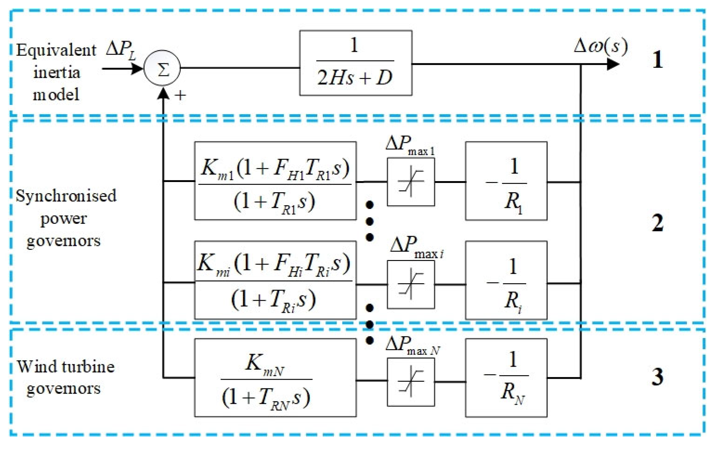
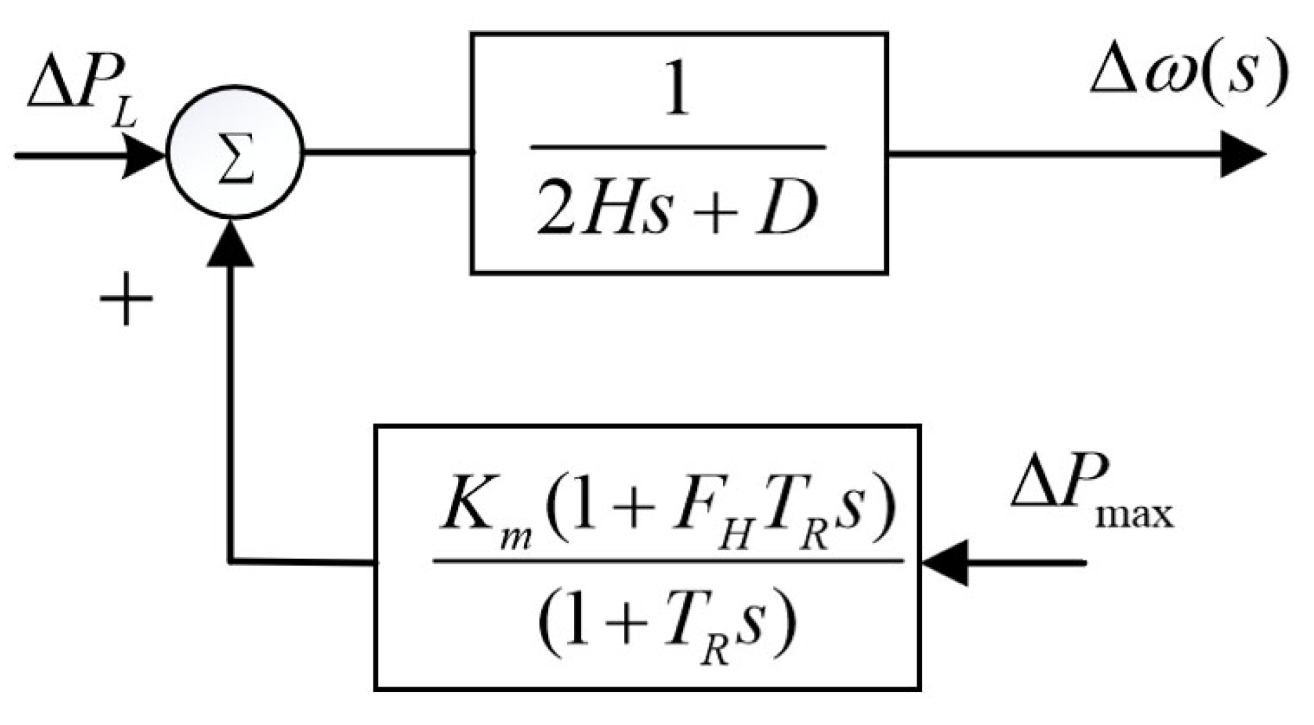
If the spatial distribution characteristics of frequency and the secondary frequency modulation link of the power supply are not considered, the SFR dynamic s-domain model after power system disturbance can be approximately represented by Figure 1.
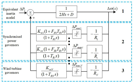
Figure 1.
SFR frequency domain model of a system containing a high proportion of wind power [24].
In Figure 1, module 1 represents the equivalent inertia model of the whole system, including the virtual inertia response of wind power, while and represent the equivalent inertia time constant and damping torque coefficient of the system, respectively; module 2 is the primary frequency modulation frequency response model of the unit based on the regulation characteristics of the thermal power unit [8], and 1~i in the parameter subscript represents the number of the hydro/thermal power unit participating in primary frequency regulation. Each unit model includes the limiting link of the speed regulator and the low-order linear transfer function module, where , , , and are the adjustment coefficient, reheat time constant, mechanical power gain factor, and high-pressure cylinder power ratio of each unit, respectively. is the limiting amplitude value of the unit speed control system, which represents the limit of the unit’s ability to participate in primary frequency regulation. If the system contains a hydraulic generator unit, according to the authors of [25], the hydraulic unit can be equivalent to a steam turbine unit with a reheat time constant of 0.5 times the water hammer effect time constant and a high-pressure cylinder power ratio of −2. Therefore, it can be used with thermal power. The units have exactly the same governor model, so the remainder of this article does not emphasize the type of unit in module 2.
This article assumes that the control method of the virtual synchronous machine used by the wind turbine involves the primary frequency regulation characteristics of the system, so module 3 is used to represent its primary frequency regulation characteristics [10].
2.2. System Single Speed Regulator SFR Frequency Domain (S-Domain) Model Based on the Multi-Machine Aggregation Method
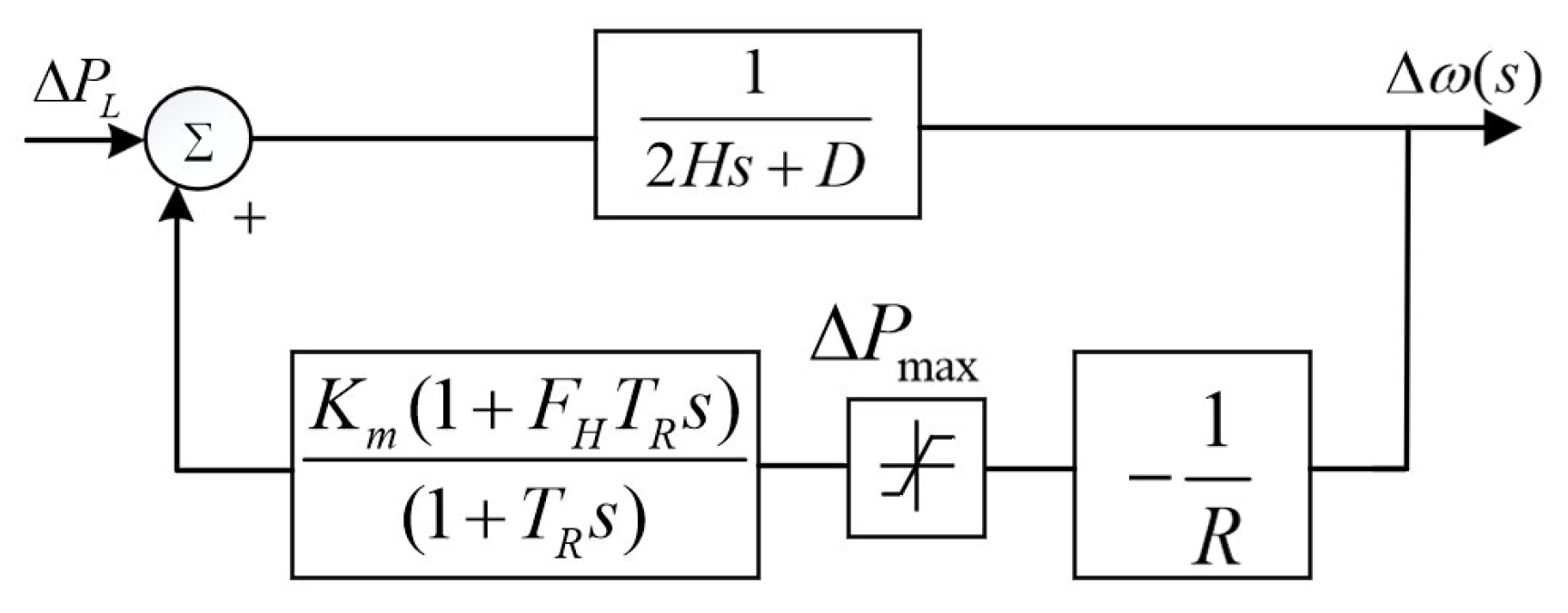
The multi-machine frequency response model is a high-order transfer function model with high computational complexity. It is difficult to directly obtain analytical frequency dynamic characteristics, which restricts the application of the multi-machine frequency response model. The conversion of a multi-machine frequency response model to a single governor model can be achieved by using the multi-machine aggregation method [26]. so as to facilitate the rapid analysis of the frequency dynamic indexes after grid disturbances. The aggregated SFR model is shown in Figure 2.
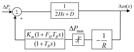
Figure 2.
Single-speed regulator frequency dynamic s-domain model based on multi-machine aggregation.
Each aggregation parameter was calculated as follows:
where and are intermediate variables; the specific calculation is as follows:
If the limiting link in Figure 2 is not considered, the s-domain expression of the system frequency response can be derived as follows [8]:
where and are, respectively, the undamped natural angular frequency and damping coefficient of the system. The specific calculation is as follows:
2.3. Single Speed Regulator SFR Frequency Domain (S-Domain) Model of the System Entering the Limiting State
If the limiting amplitude of the speed regulator of each generating unit is known, the order in which the speed regulator enters the limiting amplitude can be deduced based on the governing coefficient of each unit. On this basis, the analytical expression of the frequency response of the entire system after being disturbed is obtained through segmentation analysis and response superposition. Then a reasonable configuration of the primary frequency modulation backup is completed. However, in the primary frequency regulation backup optimization configuration problem, the limiting amplitude of the speed regulator is the variable to be optimized, so the frequency dynamic analytical expression after the system disturbance cannot be obtained through the above method.
When the speed regulator enters the limiting state, the speed regulator does not work. The system transfer function at this time is shown in Figure 3, and the dynamic s-domain model of the system at this time can be obtained, as shown in Equation (10).
The undamped natural angular frequency and damping coefficient at this time are as shown in Equations (11) and (12):

Figure 3.
System frequency dynamic s-domain model after entering the speed regulator limiting stage.
However, after entering the limiter, the system dynamic s-domain model actually has a non-zero initial state, so it is necessary to analyze the non-zero initial state on both sides of Equation (10), and we can obtain:
where is the frequency value when entering the limiting, is the frequency derivative value when entering the limiting, is the load disturbance when entering the limiting, and is the limiting amplitude when entering the limiting.
This article assumes that the power disturbance experienced by the system is a step disturbance and that the disturbance always exists. At the same time, the limiting amplitude of the speed regulator of each unit is also constant, so Equation (13) can be simplified into the following form:
Therefore, the frequency-dynamic s-domain expression when entering limiting can be expressed as follows:
2.4. Time Domain Analytical Model Considering the System Frequency of the Limiting Link
Based on Equation (15), through frequency domain–time domain transformation, the frequency response time domain analytical model of the system considering the limiting link is obtained, as shown in Equations (16)–(22):
where
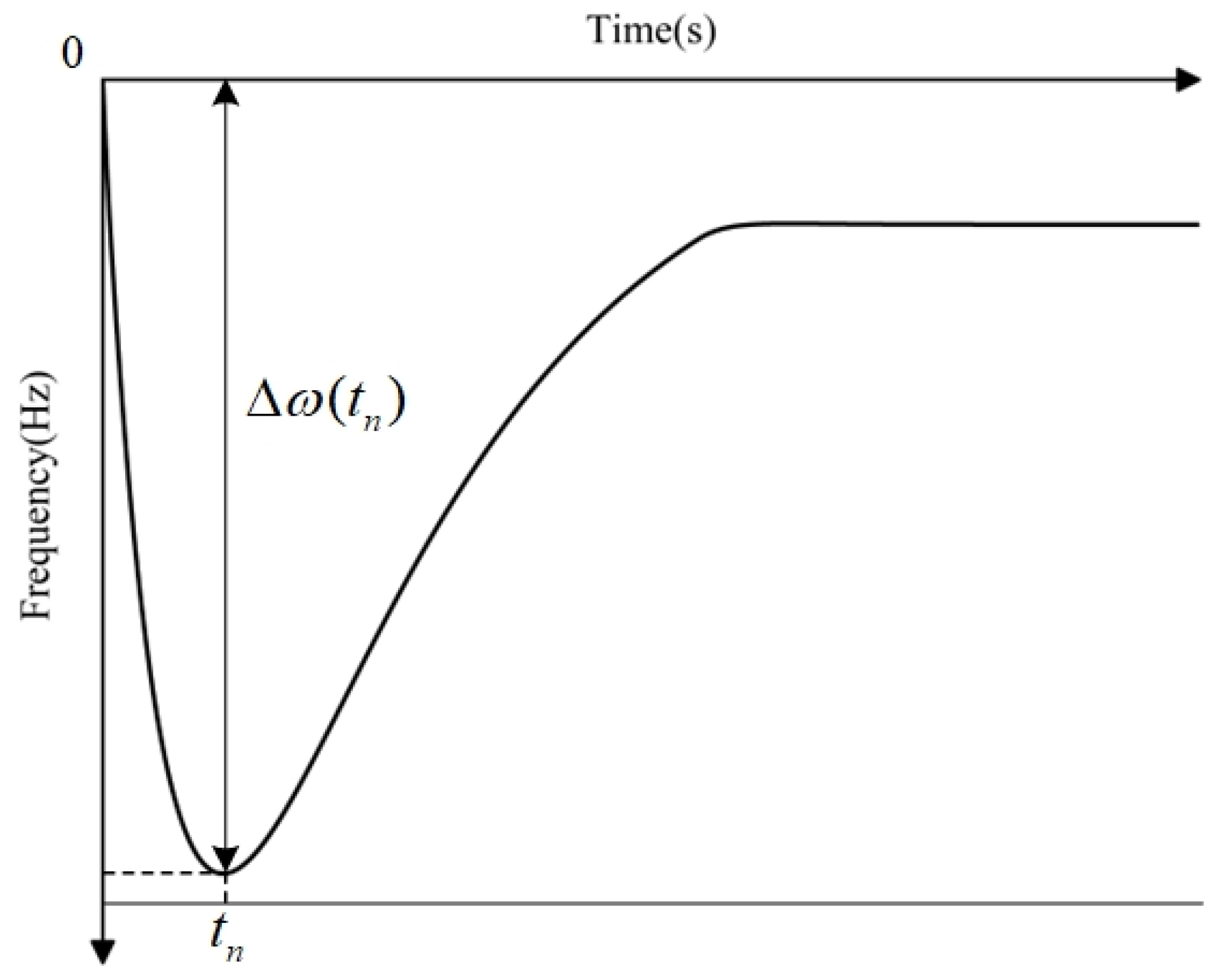
At the lowest point of frequency, the derivative of the frequency curve should be 0, as shown in Figure 4. According to the first-order optimality condition, the time when the system frequency reaches an extreme value can be obtained as follows:
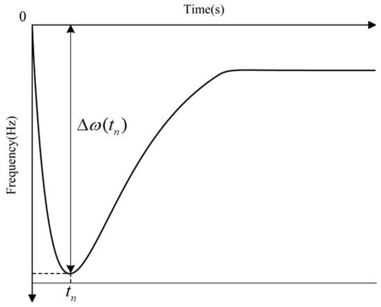
Figure 4.
Frequency response after step perturbation.
The corresponding moment is the frequency extreme value of the system:
If the disturbance conditions are known, according to Equations (16) or (24), the inertia time constant of the equivalent generator , the limiting value of the equivalent speed regulator , and the adjustment coefficient will directly affect the frequency extreme value of the system. The size and occurrence time of the points, therefore, cannot be ignored in the optimized configuration of primary frequency modulation backup.
3. Optimization of Primary Frequency Regulation Backup Configuration of New Energy Power Systems: Considering the Limiting Link
Currently, system operators only purchase fixed frequency regulation and reserve capacity in the ancillary service market (the current frequency regulation reserve capacity is 10% of the system load) to cope with frequency fluctuations. However, under the current situation of increasingly prominent frequency problems, a rigid frequency modulation backup requirement may also cause the transient frequency to exceed the safety limit, affecting the safe and stable operation of the system. In addition, the PR service provided by the unit is highly coupled with its output plan. It is necessary to incorporate the unit’s participation in the primary frequency regulation auxiliary service into the current unit output and reserve formulation process.
3.1. Optimization Model of Primary Frequency Regulation Backup Configuration of Power System
3.1.1. Objective Function
The goal of optimal configuration of PR reserve is to minimize the sum of power generation cost and primary frequency regulation reserve cost, as shown in the following formula:
where represents the number of periods; represents the total number of periods; and represent the quantity of synchronous power supply and wind power, respectively; and represent the power generation costs of synchronous power supply and wind power, respectively; and represent the backup costs of synchronous power supply and wind power, respectively; and represent the active power of synchronous power supply and wind power output, respectively; and , , , and represent the primary frequency modulation positive and negative reserve capacities of synchronous power supply and wind power; are the starting costs of synchronous power supply; and are the start and stop statuses of synchronous power supply, respectively.
3.1.2. General Constraints
The conventional constraints considered in this paper include system power balance constraints, synchronous power supply output constraints, wind power output constraints, synchronous power supply ramp constraints, synchronous power supply minimum start-up time constraints, synchronous power supply minimum downtime constraints, and system backup capacity demand constraints. For details, see Equations (26)~(36).
where , , , and are the rated capacity and minimum outputs of conventional units and wind turbines, respectively; and are the operating status of conventional units and wind turbines, respectively; and are the number of continuous on and off hours, respectively; and are the minimum start and stop times of the unit, respectively; and and are the ramp ups of a conventional power supply with lower climbing limits. It should be noted that this model does not consider the uncertainty of new energy output.
3.2. Construction of Frequency Safety Constraints Based on the SFR Time Domain Model
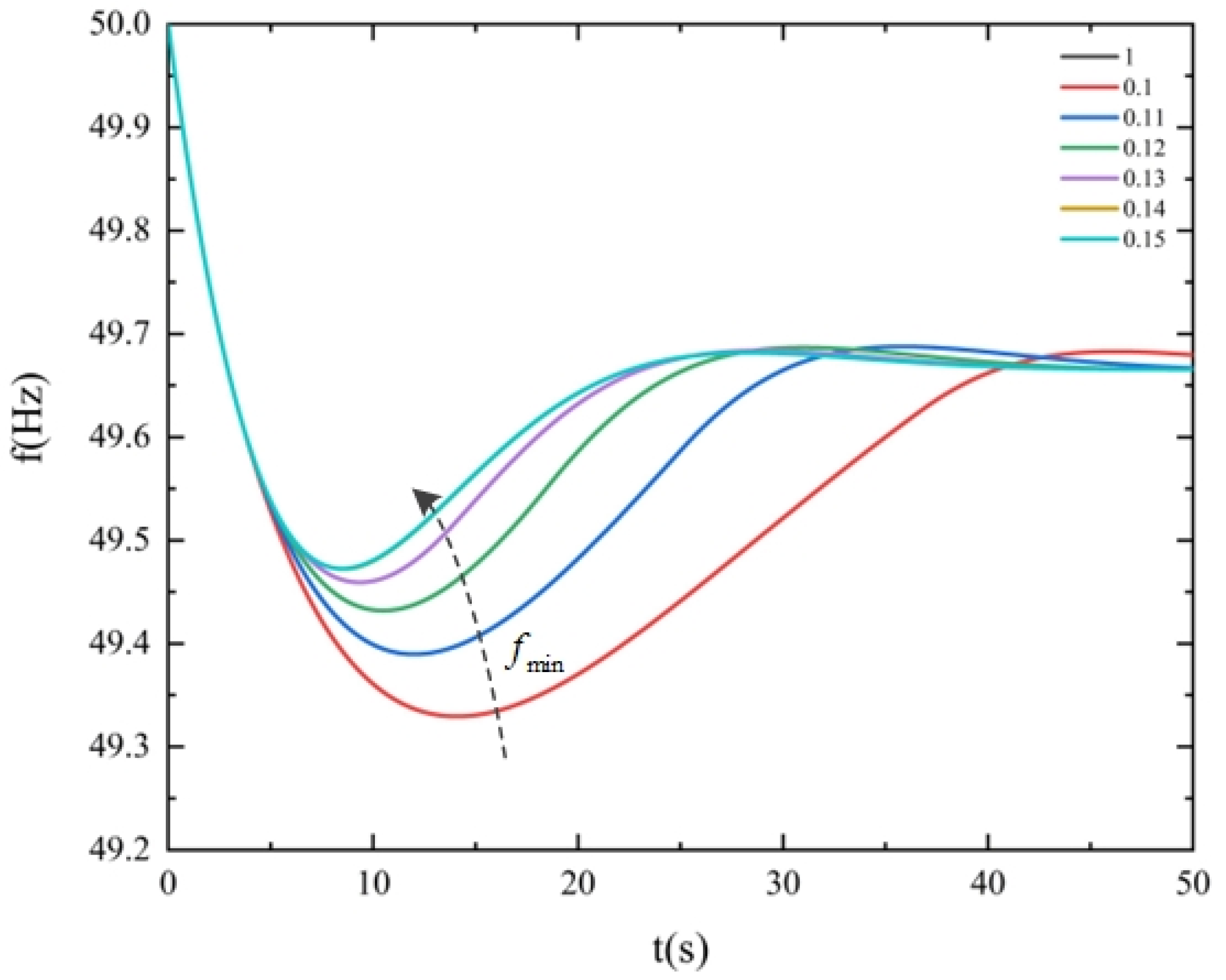
It can be seen from Equation (24) that the lowest point of the system frequency is affected by the limiting amplitude of the speed regulator. It can be seen from Equation (1) that the limiting amplitude is in the range of 0–1. When the system inertia , damping, high-pressure cylinder ratio , and the reheat time constant having been determined, the system frequency response under different limiting amplitudes is analyzed, as shown in Figure 5.

Figure 5.
System dynamic frequency response under different limiting amplitudes.
At limit amplitude values of 0.1–0.13, the system frequency nadir rises gradually with the increase of the limit value, indicating that the larger the limit amplitude is, the higher the system frequency nadir is, and the less likely it is to violate the frequency safety constraints. In the limit amplitudes of 0.14, 0.15, and 1, the system frequency response curve overlaps. That is, in the case of perturbation, the limit amplitude is greater than 0.14, the governor does not reach the limit, which is in the linear segment, and the frequency nadir no longer changes. On the one hand, the system can safely pass through the perturbation; on the other hand, it shows that the system of a PR reserve configuration exists in the case of a high degree of conservatism. At this time, the backup is not fully utilized and does not meet the economic principle of backup configuration. It can be seen that the governor limit affects the system’s frequency system maximum value and the cost of the system’s primary frequency modulation backup configuration, and the impact of the PR reserve capacity must be taken into account in the optimal dispatch of power.
Due to the system relay protection device, low-frequency load shedding device, and many other protection devices based on the rate of change of frequency () and frequency nadir, in order to avoid the frequency drop that triggers the action of the frequency protection device and ensure the system’s frequency safety, the system should meet the constraints for each time period and the frequency nadir constraints. The application of the initial value theorem of Equation (7) to obtain the rate of change of the frequency is:
Combining Equation (24), the frequency safety constraints can be obtained as follows:
where is the base frequency.
4. Two-Stage Model Solution Method Based on the L-Shape Algorithm
Due to the highly nonlinear characteristics of frequency safety constraints, it is difficult for traditional optimization toolboxes to directly solve the optimization model. The L-shape method is a method proposed by Laporte and Louveaux that uses iterative ideas to solve large-scale mixed integer programming [27], and can be applied to solve optimization problems containing nonlinear constraints.
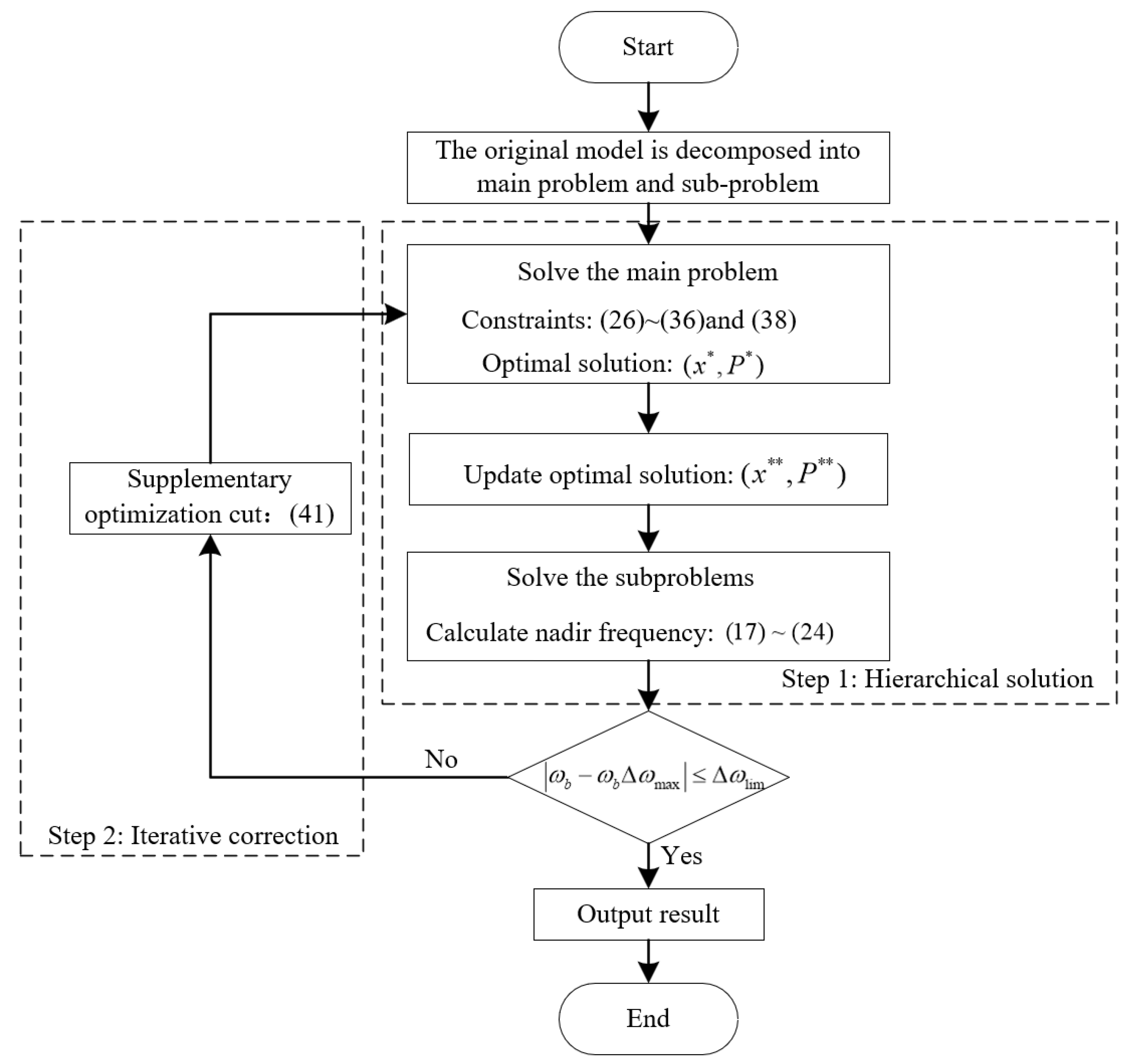
According to the two-stage iterative optimization idea of L-shape, the optimization model constructed in 2 is decomposed into a main problem and a sub-problem. The main problem is an optimization problem taking into account constraints, including the objective function (25) and constraint conditions (26)–(36) and (38); the sub-problem is a dynamic frequency minimum point constraint problem, consisting of Equations (17)–(24) and constraint conditions (39). The main problem and the sub-problem are connected through Benders cuts, so the original problem is transformed into a two-stage optimization problem, which can be solved using the L-shape method [28]. The schematic diagram of the solution process is shown in Figure 6.
- (1)
- Optimize and solve the main problem. Based on the objective function (26) and constraints (26)–(36) and (38), the start-up and shutdown plan of the unit as well as the unit output and primary frequency regulation reserve capacity can be determined for each period of the day, that is, the optimal solution (), so the system equivalent speed regulator limit in each period can be obtained as:
- (2)
- Solve the sub-problem. Calculate the frequency nadir of each period and the time to reach the lowest frequency according to Equations (17)~(24). For periods that cannot meet the lowest point frequency constraint condition (39), additional optimization cuts are required:where represents the optimal cut after update generation.
- (3)
- Use the generated optimal cut to return to the main problem and re-optimize the solution to obtain a new feasible solution (). When the sum of the output and reserve of all units in the system does not reach the maximum output of the unit, as shown in Equation (42), it means that the frequency response capability of the system can be improved at this time, and the main problem continues to increase the equivalent speed regulation of the system. The direction of the limiter is optimized until the period meets the minimum limit of the dynamic frequency.
- (4)
- Use the newly generated optimal cut to continuously iterate in the direction of increasing the system equivalent speed regulator limit, and repeat the above process until all periods meet the dynamic frequency constraints or the sum of the output and reserve of all units reaches the unit stop at maximum output.
It should be noted that when setting up a primary frequency modulation reserve, if the cost of setting up the reserve is greater than the operating cost (start-up cost, minimum output cost) of an additional thermal power unit, then according to the principle of economics, an additional thermal power unit will be opened. Raise parameters that are positively correlated with system dynamic frequency changes to reduce frequency deviations.

Figure 6.
Schematic diagram of the solution process.
Figure 6.
Schematic diagram of the solution process.
5. Example Analysis
5.1. Introduction to Simulation Examples
An improved IEEE 39 bus system is used to verify the effectiveness of the method proposed in this article. The wind power installed capacity of the test system is 2000 MW, accounting for 21.81% of the installed capacity. The steady-state operation and frequency regulation parameters of the synchronous generator and wind farm are shown in Table 1 and Table 2, respectively. This paper studies the problem of the day-ahead optimal allocation of primary frequency modulation reserve capacity. The time period is 24 h, and the time resolution of the decision variable is 1 h. The upper and lower boundaries of frequency stability are set to 50.5 Hz and 49.5 Hz, respectively, and the upper and lower steps of the frequency change rate are ±0.5 Hz/s. Following the description of disturbances in the operating mode optimization problem considering frequency stability constraints in literature [14], the disturbance type is set to a sudden increase in active load with an amplitude of 10% of the maximum load. The load and wind power prediction curves are shown in Figure 7.

Table 1.
Power supply steady-state parameters.
Table 2.
Power supply frequency regulation parameters.
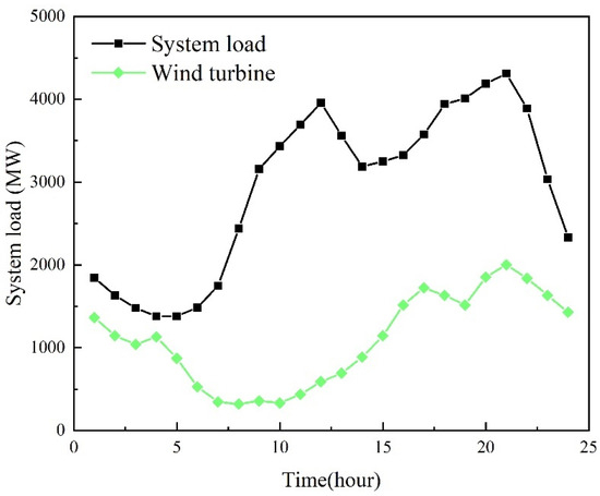
Figure 7.
Load and wind power forecast curves.
In order to verify the effectiveness of the model in this article and the impact of the post-disturbance frequency analysis method on the primary frequency modulation backup configuration, three comparison schemes are set up.
Case 1: Regardless of frequency stability constraints, units participating in frequency regulation are forced to reserve 10% of their maximum load as primary frequency regulation positive and negative reserves in each period.
Case 2: Considering the frequency stability constraint, the limiting link is considered in the traditional SFR model, but the speed regulator is forced to be in the linear segment [11], and the units participating in frequency regulation in each period are forced to reserve 10% of the maximum load as the primary frequency regulation positive, negative reserve.
Case 3: Combined with the model of this article, consider the frequency stability constraints and the limiting effect of the speed regulator.
5.2. Analysis of Results under Different Scenarios
5.2.1. Primary Frequency Modulation Backup Optimization Economic Indicators
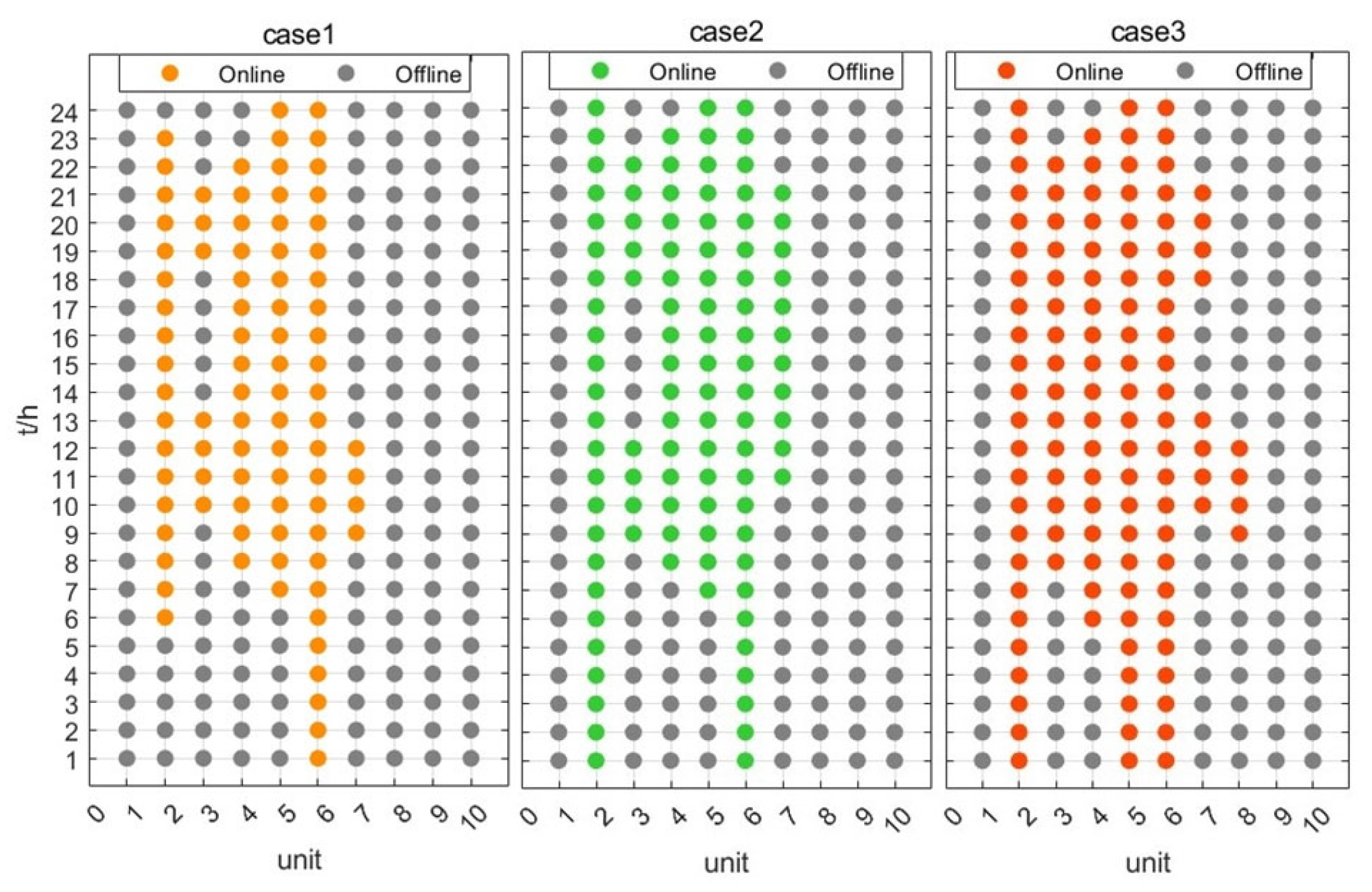
Based on the above various models, the optimization calculation results of the primary frequency regulation reserve of the power system with a high proportion of wind power are shown in Figure 8, Figure 9 and Figure 10, and the operating costs of the system are shown in Table 3.
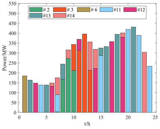
Figure 8.
Case 1 frequency modulation positive standby configuration results.
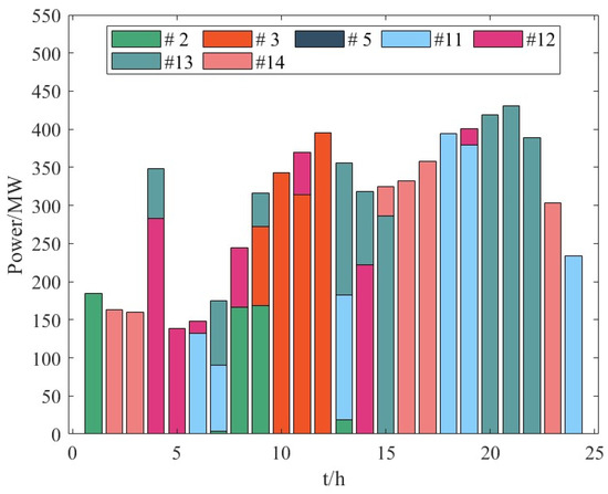
Figure 9.
Case 2 frequency modulation positive standby configuration results.
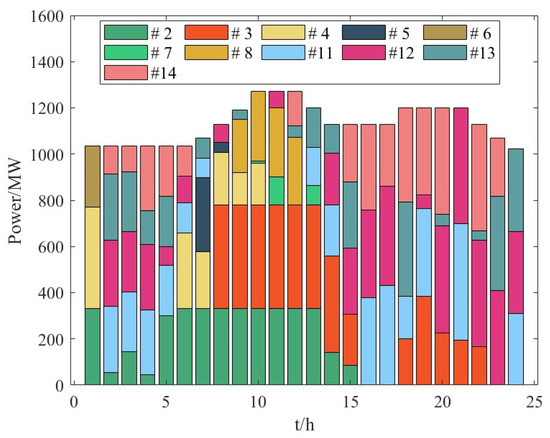
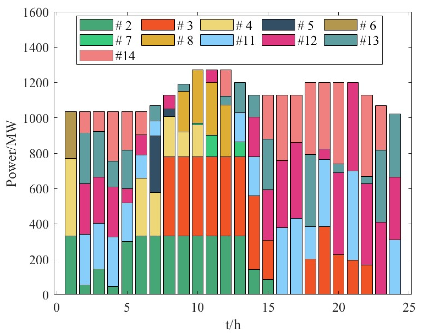
Figure 10.
Case 3 frequency modulation positive standby configuration results.
Table 3.
Comparison of running results of various schemes.
- (1)
- Case 1: This model allocates a primary frequency regulation reserve to each power supply in the powered-on state. Although cost factors are taken into consideration when configuring the reserve, and the frequency modulation reserve is allocated to units with lower reserve costs, the adequacy of the reserve is not considered and is of little reference.
- (2)
- Case 2: Considering the frequency change rate constraint, the number of systems turned on will inevitably increase, and the power generation cost of the system will inevitably change. This scheme combines the lowest frequency constraint obtained by the authors of [11], but requires the speed regulator to work in a linear state and still reserves a proportional frequency modulation for backup. For this reason, the frequency modulation reserve left by each power supply is still relatively large. Compared with option 1, the cost of one frequency modulation reserve is reduced by 0.39%, and the total operating cost is reduced by 0.38%.
- (3)
- Case 3: The model considers the frequency stability constraints and the limiting link of each power supply speed regulator. After aggregating the parameters, combined with the judgment that the lowest frequency point will inevitably appear in the speed regulator limiting stage, the primary frequency modulation is realized. Optimization of spare capacity configuration. Since the frequency limit constraint is more stringent, the primary frequency modulation reserve required by the system is bound to increase. Compared with option 1, the cost of the primary frequency modulation reserve increases by 15.15%, and the total operating cost increases by 22.53%. Compared to Case 2, the cost of the primary frequency modulation reserve increased by 15.6%, and the total operating cost increased by 23%. Since the backup is distributed among the units already turned on, after accounting for the limiting link, if the cost of the backup configuration is greater than the operating cost of turning on another unit in the system, the choice is made to turn on the new unit. Comparing Figure 8, Figure 9 and Figure 10, it can be seen that Case 3 has a high demand for frequency modulation backup, which leads to the need to switch on new units in addition to the backup provided by the wind turbines. For example, at 9–12, Unit 8 in Case 3 is operational and provides a percentage of the standby.
5.2.2. System Frequency Stability Verification under Large Disturbance Conditions
The synchronous power supply start and stop modes of the three schemes are shown in Figure 11. According to the start–stop plan, the simulation calculation of each plan and each period is shown in Figure 12. As can be seen from Figure 12, the number of startups in Case 1 is small, its frequency change rate constraints in the 1–2 period and the 15–24 period do not meet the standards, and the system frequency response capability is low. When considering the frequency change rate constraint, the number of synchronous power supply startups in the system increases. This is because the frequency change rate of the system is affected by the inertia level of the system. The more synchronous units are started, the higher the inertia level of the system, and the less likely it is to violate frequency change rate constraints.
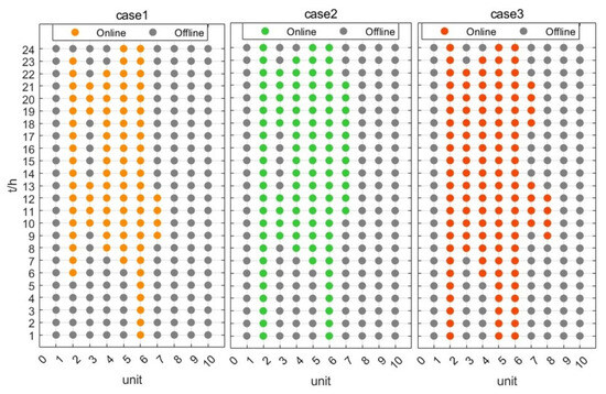
Figure 11.
Start-up and shutdown situations of traditional units with three cases.
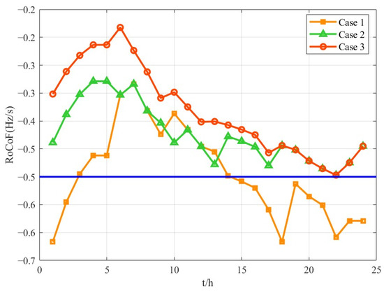
Figure 12.
Frequency change rate chart of three cases.
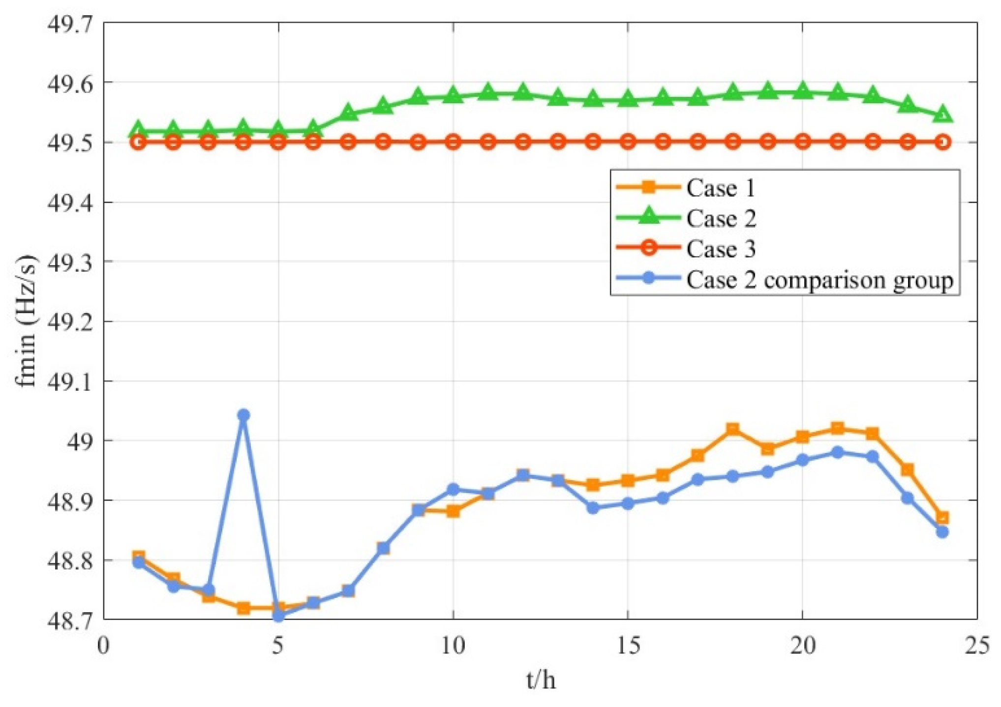
According to the simulation results, the lowest frequency point in each period is calculated, and the results in Case 2 are brought into the solution model of the lowest frequency point in this article, as shown in Figure 13. The lowest frequency points in all periods in Scheme 1 are all over the limit, and its frequency modulation backup cost is the highest. Its backup configuration strategy cannot meet the frequency minimum point constraints under extremely large disturbance conditions. In Scheme 2, the lowest frequency point constraint does not consider the influence of amplitude limiting, and the lowest frequency points are all higher than 49.5 Hz, which satisfies the lowest point constraint obtained from [11]. However, when the results in Case 2 are brought into the frequency nadir calculation model in this paper, considering the limiting link, its frequency nadir is not satisfied for all time periods and is given as a blue curve in Figure 13. It indicates that its PR standby configuration strategy still fails to meet the frequency constraint requirements under the actual governor operating characteristics. Meanwhile, the lowest point of frequency at four moments is higher compared with other times. Combined with Figure. 9, it can be seen that the PR standby capacity is larger at this time, and the lowest point of frequency is higher, which further verifies that increasing the PR standby capacity can enhance the frequency security of the system. From the red curve in Case 3, it can be seen that the frequency minimum point of this paper’s model under extreme disturbance conditions exactly meets the frequency stability constraints; that is, at this point in time, the PR backup is fully utilized, reflecting the standby configuration results of the economy.

Figure 13.
Frequency nadir of the 3 cases.
6. Conclusions
This paper combines the system frequency response model, considering the limiting link, into the primary frequency regulation optimization configuration problem of the power system connected to the large-scale wind power grid. Aiming at the high-order nonlinear problem of frequency constraints, a primary frequency regulation reserve capacity is proposed as the master sub-problem of the optimal cut connection. In the two-stage iterative method, the conclusions are as follows:
- (1)
- The constraints established take into account the impact of governor limiting on frequency response, making the estimation of the frequency modulation capability of the system more accurate. This further ensures the effectiveness of the obtained unit combination and primary frequency regulation capacity configuration plan, thereby effectively ensuring the frequency stability of the new energy power system.
- (2)
- Due to the existence of high-order nonlinear terms in the system frequency and extreme point constraints after disturbance, a two-stage iterative solution method based on L-shape is proposed to decompose the nonlinear optimization model into main sub-problems. This method effectively reduces the solution cost of the primary frequency modulation backup configuration model.
At present, this article only considers the impact of the power supply speed regulator limiting link (i.e., primary frequency regulation backup) on the system frequency extreme point after the disturbance and has not yet considered the impact of the uncertainty of new energy output. At the same time, this article also lacks research on how the primary frequency modulation capacity after disturbance can be more reasonably applied in the frequency modulation process. In addition, the advantages of artificial intelligence technology in dealing with optimization problems containing uncertainty and related nonlinearities are gradually coming to the fore, and how it can be used in PR standby allocation problems will also become the subsequent research direction of this paper.
Author Contributions
Conceptualization, M.W. and C.X.; methodology, C.X.; software, C.X.; validation, M.W. and C.X.; formal analysis, C.X.; investigation, C.X.; resources, M.W.; data curation, C.X.; writing—original draft preparation, C.X.; writing—review and editing, C.X.; visualization, C.X.; supervision, M.W.; project administration, M.W.; funding acquisition, M.W. All authors have read and agreed to the published version of the manuscript.
Funding
This research was funded by [Qingpu Power Supply Company State Grid Shanghai Municipal Electric Power Company] grant number [B30934230002] and the APC was funded by [B30934230002].
Data Availability Statement
The data presented in this study are available in [24].
Conflicts of Interest
The authors declare no conflict of interest.
References
- Zhang, Z.Y.; Zhang, N.; Du, E.S.; Kang, C.Q.; Wang, Z.D. Review and Countermeasures on Frequency Security Issues of Power Systems with High Shares of Renewables and Power Electronics. Proc. CSEE 2022, 42, 1–25. [Google Scholar]
- Li, Z.W.; Wu, X.L.; Zhuang, K.Q.; Wang, L.; Mu, Y.C.; Li, B.J. Analysis and Reflection on Frequency Characteristics of East China Grid After Bipolar Locking of “9·19” Jinping-Sunan DC Transmission Line. Autom. Electr. Power Syst. 2017, 41, 149–155. [Google Scholar]
- Sun, H.D.; Xu, T.; Guo, Q.; Li, Y.L.; Lin, W.F.; Yi, J.; Li, W.F. Analysis on Blackout in Great Britain Power Grid on August 9th, 2019 and Its Enlightenment to Power Grid in China. Proc. CSEE 2019, 39, 6183–6191. [Google Scholar]
- GB/T 40595-2021; Guide for Technology and Test on Primary Frequency Control of Grid-Connected Power Resource. State Administration for Maket Regulation: Beijing, China, 2021.
- Wang, M.J.; Guo, J.B.; Ma, S.C.; Wang, T.Z.; Zhang, X.; Luo, K.; Wang, G.Z. Review of Transient Frequency Stability Analysis and Frequency Regulation Control Methods for Renewable Power Systems. Proc. CSEE 2023, 43, 1672–1693. [Google Scholar]
- Wen, Y.; Chung, C.Y.; Liu, X.; Che, L. Microgrid Dispatch with Frequency-Aware Islanding Constraints. IEEE Trans. Power Syst. 2019, 34, 2465–2468. [Google Scholar] [CrossRef]
- Javadi, M.; Gong, Y.; Chung, C.Y. Frequency Stability Constrained Microgrid Scheduling Considering Seamless Islanding. IEEE Trans. Power Syst. 2022, 37, 306–316. [Google Scholar] [CrossRef]
- Anderson, P.M.; Mirheydar, M. A low-order system frequency response model. IEEE Trans. Power Syst. 1990, 5, 720–729. [Google Scholar] [CrossRef]
- Chan, M.L.; Dunlop, R.D.; Schweppe, F. Dynamic Equivalents for Average System Frequency Behavior Following Major Distribances. IEEE Trans. Power App. Syst. 1972, 91, 1637–1642. [Google Scholar] [CrossRef]
- Shintai, T.; Miura, Y.; Ise, T. Oscillation Damping of a Distributed Generator Using a Virtual Synchronous Generator. IEEE Trans. Power Deliv. 2014, 29, 668–676. [Google Scholar] [CrossRef]
- Zhang, Z.; Du, E.; Teng, F.; Zhang, N.; Kang, C. Modeling Frequency Dynamics in Unit Commitment with a High Share of Renewable Energy. IEEE Trans. Power Syst. 2020, 35, 4383–4395. [Google Scholar] [CrossRef]
- Shen, J.K.; Li, W.D.; Li, Z.W.; Zeng, H.; Zheng, H.C. Unit Commitment of Power System with High Proportion of Wind Power Considering the Deadband and Limiter of Primary Frequency Response. Power Syst. Technol. 2022, 46, 1326–1334. [Google Scholar]
- Ahmadi, H.; Ghasemi, H. Security-Constrained Unit Commitment with Linearized System Frequency Limit Constraints. IEEE Trans. Power Syst. 2014, 29, 1536–1545. [Google Scholar] [CrossRef]
- Paturet, M.; Markovic, U.; Delikaraoglou, S.; Vrettos, E.; Aristidou, P.; Hug, G. Stochastic Unit Commitment in Low-Inertia Grids. IEEE Trans. Power Syst. 2020, 35, 3448–3458. [Google Scholar] [CrossRef]
- Li, J.M.; Qiao, Y.; Lu, Z.X.; Ma, W.; Cao, X.; Sun, R.F. Integrated Frequency-constrained Scheduling Considering Coordination of Frequency Regulation Capabilities from Multi-source Converters. J. Mod. Power Syst. Clean Energy 2024, 12, 261–274. [Google Scholar] [CrossRef]
- Lagos, D.T.; Hatziargyriou, N.D. Data-Driven Frequency Dynamic Unit Commitment for Island Systems with High RES Penetration. IEEE Trans. Power Syst. 2021, 36, 4699–4711. [Google Scholar] [CrossRef]
- Zhang, Y.; Cui, H.; Liu, J.; Qiu, F.; Hong, T.; Yao, R.; Li, F. Encoding Frequency Constraints in Preventive Unit Commitment Using Deep Learning with Region-of-Interest Active Sampling. IEEE Trans. Power Syst. 2022, 37, 1942–1955. [Google Scholar] [CrossRef]
- Shen, Y.K.; Wu, W.C.; Wang, B.; Yang, Y.; Lin, Y. Data-driven Convexification for Frequency Nadir Constraint of Unit Commitment. J. Mod. Power Syst. Clean. Energy 2023, 11, 1711–1717. [Google Scholar] [CrossRef]
- Liu, L.K.; Hu, Z.C.; Wen, Y.L.; Ma, Y.X. Modeling of Frequency Security Constraints and Quantification of Frequency Control Reserve Capacities for Unit Commitment. IEEE Trans. Power Syst. 2024, 39, 2080–2092. [Google Scholar] [CrossRef]
- Ge, X.L.; Liu, Y.; Fu, Y.; Jia, F. Distributed Robust Unit Commitment Considering the Whole Process of Inertia Support and Frequency Regulations. Proc. CSEE 2021, 41, 4043–4058. [Google Scholar]
- Wang, X.; Ying, L.M.; Lu, S.P. Joint Optimization Model for Primary and Secondary Frequency Regulation Considering Dynamic Frequency Constraint. Power Syst. Technol. 2020, 44, 2858–2867. [Google Scholar]
- Zhou, X.Y.; Liu, R.; Bao, F.Z.; Zhang, M.Z.; Wang, H.X.; Li, W.D. Joint Optimization Model for Hundred-megawatt-level Energy Storage Participating in Dual Ancillary Services Dispatch of Power Grid. Autom. Electr. Power Syst. 2021, 45, 60–69. [Google Scholar]
- Ye, J.; Lin, T.; Zhang, L.; Bi, R.Y.; Xu, X.L. Isolated Grid Unit Commitment with Dynamic Frequency Constraint Considering Photovoltaic Power Plants Participating in Frequency Regulation. Trans. China Electrotech. Soc. 2017, 32, 194–202. [Google Scholar]
- Yang, M.Q.; Wang, C.; Ge, C.Y.; Bi, T.S.; Wang, X.G.; Zhou, Z. Primary Frequency Regulation Reserve Procurement of Renewable Energy Power System Considering Multiple Damping States and Governor Limiters. Proc. CSEE. 2024, 44, 147–160. [Google Scholar]
- Ni, Y.X.; Chen, S.S.; Zhang, B.L. Theory and Analysis of Dynamic Power Systems, 1st ed.; Tsinghua University Press: Beijing, China, 2002; pp. 76–78. [Google Scholar]
- Shi, Q.; Li, F.; Cui, H. Analytical Method to Aggregate Multi-Machine SFR Model with Applications in Power System Dynamic Studies. IEEE Trans. Power Syst. 2018, 33, 6355–6367. [Google Scholar] [CrossRef]
- Lee, Y.Y.; Baldick, R. A Frequency-Constrained Stochastic Economic Dispatch Model. IEEE Trans. Power Syst. 2013, 28, 2301–2312. [Google Scholar] [CrossRef]
- Golshani, A.; Sun, W.; Zhou, Q.; Zheng, Q.P.; Hou, Y. Incorporating Wind Energy in Power System Restoration Planning. IEEE Trans. Smart Grid 2019, 10, 16–28. [Google Scholar] [CrossRef]


Disclaimer/Publisher’s Note: The statements, opinions and data contained in all publications are solely those of the individual author(s) and contributor(s) and not of MDPI and/or the editor(s). MDPI and/or the editor(s) disclaim responsibility for any injury to people or property resulting from any ideas, methods, instructions or products referred to in the content. |
© 2024 by the authors. Licensee MDPI, Basel, Switzerland. This article is an open access article distributed under the terms and conditions of the Creative Commons Attribution (CC BY) license (https://creativecommons.org/licenses/by/4.0/).