1. Introduction
The transport sector accounts for a large contribution to greenhouse gas emissions. In this context, electric vehicles (EVs) are emerging as one of the solutions that will help the European Union (EU) achieve its climate neutrality targets [
1]. Thus, the EU has taken the measure of banning the sale of new petrol and diesel cars from 2035 [
2,
3]. In the first quarter of 2023, over 2.3 million EVs were sold worldwide, 25% more than in the same period the precedent year [
4]. To cope with this growth, EV chargers will have to be installed every 60 km by 2026 [
5].
According to [
6], uncontrolled deployment of EVs would increase peak electricity demand by 35% to 51%. Without proper control, the high penetration of EVs will widen the gap between peak and off-peak loads on the grid [
7]. This fact could overload distribution lines and transformers, leading to higher grid losses and reduced equipment lifetime [
8].
However, coordinating the charging of EVs could also offer significant flexibility [
9]. One solution involves using renewable energy sources (RES) for EV charging. By scheduling charging during times when RES is available, more RES is integrated into the grid and the gap between peak and off-peak power is reduced [
9]. This way, local solar energy self-consumption holds the potential to emerge as a multifaceted solution.
When using EVs as flexible loads to help reduce grid operation issues, it is essential to manage the charging pattern in a controlled manner. EV control systems that intend to ensure an acceptable charging profile can be classified into two main types: direct and indirect control [
10]. Direct control involves acting on the load patterns directly by controlling the charging power. One of the drawbacks of direct control systems is the high communication and computational infrastructure required. On the other hand, indirect control is based on encouraging EV users to adapt their charging patterns. The most common method of influence is through charging tariffs. There are several charging tariff systems, such as real-time pricing (RTP), critical peak pricing (CPP), and time-of-use (ToU) charging. In the RTP solution, prices for each time slot are announced shortly before the interval starts. Although this scheme is very efficient due to its dynamic nature, it requires a large information and communication technology (ICT) infrastructure. Furthermore, it requires substantial user participation [
11]. In the case of CPP, extremely high prices are charged for occasions where peak demand is very high [
12]. This type of pricing can be associated with others, whereas in ToU strategies, different fixed windows in the day are related to different fixed rates [
13]. ToU charging system is the most widely used because of the simplicity of implementation [
10,
14].
Several papers have studied how EVs can benefit the electricity grid [
15]. In [
16], pricing mechanisms to incentivize EV users to shift their charging to fill the off-peak zones are proposed. The authors highlight that by using ToU-based charging, EV users would choose to charge the vehicle at the beginning of the cheapest zone, causing a new consumption peak. For this reason, the authors propose two charging mechanisms: one non-cooperative and the other cooperative, which consider the charging schedules of the vehicles that have already arrived. In the non-cooperative scenario, each EV schedules its own charging without cooperating with the other EVs, while in the cooperative scenario, all EVs are controlled by an aggregator. In [
17], a day-ahead dispatch strategy is proposed for EVs considering the carbon quota. In addition, this strategy can provide peak shaving and valley-filling services.
Other works have studied the synergy between photovoltaic (PV) energy and EV charging. In [
18,
19], an indirect control approach presents a dynamic pricing system based on the Stackelberg game for an EV charging station associated with a PV system. The Stackelberg equilibrium seeks a win–win situation, reducing the cost for users and increasing the profit of the charging station. In [
19], the charging station sets an appropriate selling price to maximise its profit. Then, the Stackelberg equilibrium is solved considering the user’s criteria, and the prices are determined by the charging station.
There are also studies examining the role of EVs in increasing the PV self-consumption rate (SCR). Studies in [
20,
21] present improvements in PV self-consumption and self-sufficiency using batteries and EVs without applying any control. For instance, in [
20], households with PV generation exhibited a SCR of 26% without storage, 59% with an EV, and 31% with batteries sized for that case study. Conversely, works [
22,
23] implement a direct control with the objective of maximising the SCR. In [
22], direct control is used to define the charging pattern of EVs considering them as a flexible charging source, and in the case of vehicle to grid (V2G) as a storage device. In this work, three charging algorithms are proposed. The first algorithm uses real-time information, the second incorporates V2G technology, and the third is an optimisation algorithm using predictions for both demand and production, taking into account V2G technology. The results present a SCR of 49% for the uncontrolled case, 62% with the first algorithm, 79% with the second, and 87% with the third. The study conducted in [
23] presents a combination of smart metering and smart charging that helps local energy communities increase self-consumption. A case with four consumers and a prosumer is studied. In the scenario without EVs, one-fifth of the PV energy is consumed, while with smart metering and EVs, the SCR is increased by 45%. In [
24], a distributed and centralised smart charging scheme for EVs in residential buildings with PV systems is presented. The aim of smart charging is to minimise net load variability, thereby increasing self-consumption and reducing consumption peaks. In the centralised charging scheme, a central unit determines the charging time and power for a fleet of EVs, whereas, in the distributed charging approach, charging decisions are made at the user level. The proposed smart charging schemes consider EV energy demand, arrival and departure times, and predictions of building consumption and PV production.
Considering the state-of-the-art study conducted, there are no studies that assess the improvement of PV SCR through the use of indirect control systems in EV charging.
The work presented in this paper proposes three charging tariff schemes based on temporary PV surpluses in a real PV collective self-consumption (CSC) project in Aduna (Basque Autonomous Community, Spain). All three tariff systems (TS) share the same objective: to influence user behaviour in shifting the timing of EV charging to increase the consumption of local PV energy, and thus indirectly decrease the charging cost of the EV users.
The following hypotheses were considered:
- I.
EV users prefer to charge their vehicles when prices are lower. Therefore, if reduced prices are offered during PV surplus hours, users will adjust their charging times.
- II.
The resolution in the control of EV charging power considered in this article is ideal.
The two main contributions of the research study are as follows:
The design of indirect control EV charging is based on temporary PV surplus, with the main objective of increasing the SCR of a real PV CSC project.
A detailed description of the design of three TSs for EV charging, which can be easily replicated and adjusted to any case.
It is also worth highlighting that these TSs would promote the development of EVs, which is the aim of the Aduna town council, the owner of the PV panels and EV chargers.
The rest of this document is organised as follows.
Section 2 presents the case study and the data used. In
Section 3, the proposed three TSs are explained. Numerical results and discussion are provided in
Section 4. Finally, the last section concludes this article.
2. Case Study
The three TSs proposed in this work were simulated with real historical data collected from the PV CSC project. This project takes place in the municipality of Aduna, located in the Basque Country, Spain. There are eight consumption points associated with the CSC project. One of them is a public EV charging point. For administrative reasons, the PV panels with a capacity of 62.4 kWp were not yet installed during this study.
The mentioned data can be divided into three groups: the data related to the eight consumption points, the data on the public EV charging station obtained from the Charge and Parking application, and the data related to PV power generation.
The consumption of the seven points (all except the EV charger) is considered to be the basic consumption for this case study. This consumption is used to obtain the PV surplus by calculating the difference between PV production and basic consumption. All proposed TSs are based on the PV surpluses. In this document, these surpluses are directly calculated by subtracting the basic consumption from the PV generation. However, when implementing the TSs in real time, the energy management system (EMS) will use the day-ahead forecasts of both PV production and consumption (as carried out in [
25,
26]).
The consumption historical data were recorded hourly and were available for the last 3 years. However, since the public charging point was not installed until November 2021, the simulations considered data obtained between November 2021 and April 2022, the same period as for the EV charging data.
On the other hand, the sampling time was reduced from 1 h to 10 min (the sample time corresponding to PV generation), with the objective of producing more accurate simulations. In this way, the EV charging time was more closely adjusted to the real charging time. To perform the change in the sampling time, the value of the power consumed over one hour was used in the six intervals that constitute one hour.
The public EV charging station is a 22 kW three-phase charger with two connectors. Regarding the EV charging data, the following information was obtained using the Charge and Parking application: the time at which an EV was connected and disconnected, the EV brand and model, and the total energy consumed for each charge. By knowing the EV brand and model, it was possible to check and record the maximum charging power for each EV. It should be noted that not all EV models charge at the same power. Among the 23 EV models registered in the Charge and Parking application, the most common maximum charging power values were 3.7 kW, 7.2 kW, and 11 kW. These maximum power values were used in the design of TS1 and 2.
Regarding PV data, they were obtained using local historical solar irradiance data for the simulation period, from the Basque Meteorological Agency, Euskalmet [
27], with a sampling interval of 10 min. PV production was estimated by multiplying the irradiation by the peak power of the PV panels and applying a correction factor to account for efficiency.
3. Proposed Pricing Methods
The following section describes the three proposed TSs to influence the EV user’s charging pattern.
Although the three TS algorithms share the same objective, their rules are different. TS1 and 2 are indirect controls. TS1 is the least complex: when the PV surplus exceeds 7 kW, a lower price is offered to EV users to encourage charging at that time. On the other hand, TS2 is more personalised and is offered when the PV surplus exceeds different levels corresponding to the different charging power of EVs. Finally, TS3 is based on a hybrid control. In this TS, a cheaper charging price is always offered when there is a PV surplus, regardless of the amount, and the EV on-board battery management system (BMS) and the charger modify the charging power depending on the surplus at any given time, without consuming energy from the grid.
The three proposed TSs offer a cheaper price than the market price to encourage charging at the most opportune times. However, when there is no surplus, the market price is offered.
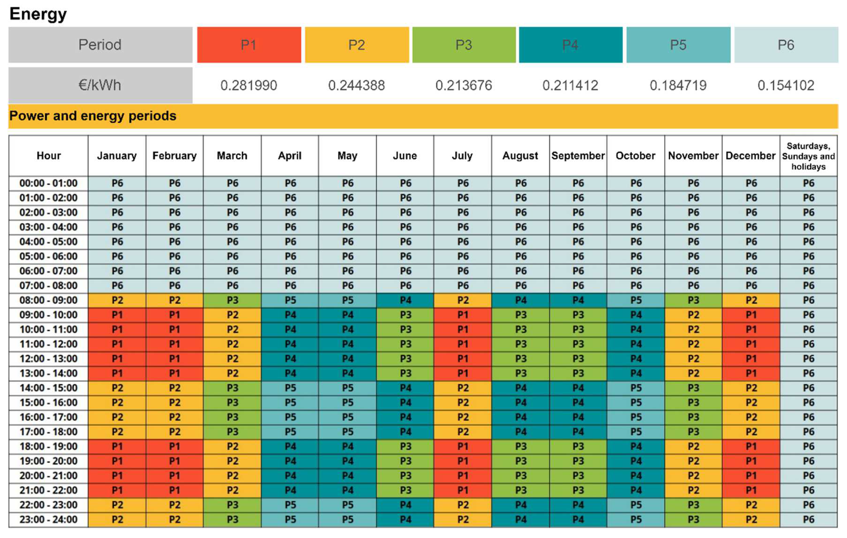
3.1. Market Tariff Used as Base Tariff
The market tariff used as the base tariff for the three TSs is one of the GoiEner cooperatives [
28], specifically the 3.0 TDVE tariff, which is tailored for public charging points. The 3.0 TDVE tariff has different prices per hourly slot, with modifications each month, as described in
Figure 1. There are six periods with different energy and power rates used in the various hourly slots. Regarding the GoiEner’s self-consumption compensation price, it is 0.0839 EUR/kWh. The compensation price is the price at which the PV panel owner is compensated for injecting locally generated PV energy into the grid that has not been instantaneously consumed. Charging and compensation prices are reviewed every trimester.
To conclude, the three proposed TSs offer the compensation price (0.0839 EUR/kWh) when the specific conditions of each TS are fulfilled. When the conditions are not met, the charging price is the market price for the corresponding time slot and month.
3.2. Tariff System 1
The first TS is the simplest one. Whenever the PV surplus exceeds 7 kW, the reduced price is offered. There are two main reasons why the threshold is set at 7 kW. On the one hand, if the threshold is very low, by offering the reduced price, EVs would consume more from the grid and less from the surplus, as the users would charge their EVs when the surplus is lower. On the other hand, the average maximum charging power of all registered EVs is around 7 kW.
The main disadvantage of this TS is that there are occasions when the surplus is less than 7 kW and is not used.
To calculate SCRs that would be obtained with the implementation of TS1, a simulation was carried out based on the historical data presented in
Section 2. The simulator was coded in MATLAB
® software 9.13.0.2166757 (R2022b) Update 4. The simulation was performed for each day where EVs were charged during the above-mentioned six months. The EVs considered in the simulation on a given day were processed in the order of original arrival at the charging point. Additionally, since charging system 1 is an indirect control, once the EV had started to charge in the simulation (when the reduced price was offered), the EV was charged at its maximum power until it was fully charged, even though after a while the reduced price was no longer offered. This process was considered to be the most realistic.
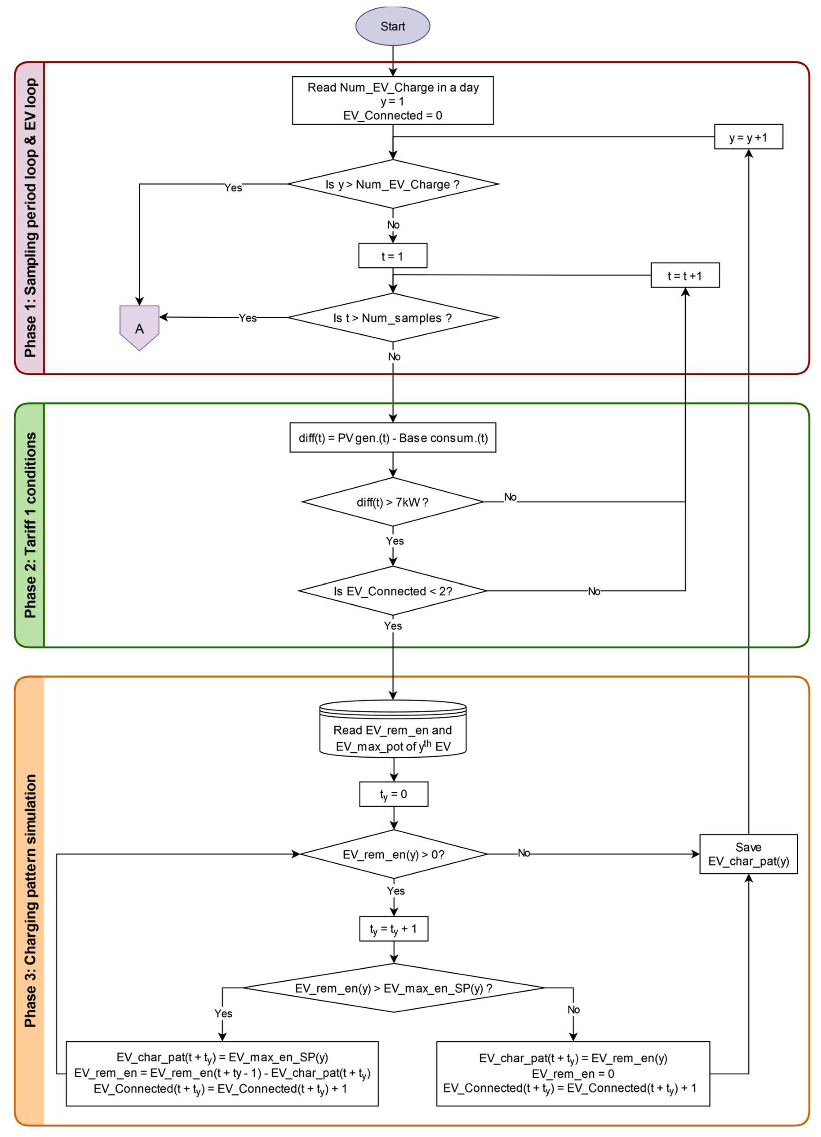
The flow chart in
Figure 2 describes the simulation process for one day under the influence of TS1. The diagram can be divided into three phases. The first phase is composed of the two main loops, which ensure that all EVs and all sampling periods of the day are analysed. It starts by detecting how many EVs were charged that day (variable
Num_EV_Charge). The simulation starts by analysing the first EV of the day, so the index
y takes the value 1 (
y = 1). When the charge of the first EV is simulated, index
y is incremented to 2 to consider the next EV of the day. When
y is greater than
Num_EV_Charge, it means that all EVs have been simulated and therefore the simulation of the EV charging pattern ends, leading to Figure 7’s flow chart (linked to connector A) where the charging cost is calculated.
Next, the first sampling period (t = 1) is analysed. Given that in the simulation the sample time is 10 min, the first sampling period, t = 1, starts at 00:10. The index t is incremented every new period until it reaches a value of Num_samples, 144 (00:00). When t is greater than Num_samples, the simulation ends, leading to Figure 7’s flow chart.
The second phase analyses whether the conditions are met to offer the reduced price according to TS1. For this purpose, the difference between the consumption and the PV production at time t (diff(t)) is calculated. If diff(t) exceeds 7 kW, the reduced price is offered, and therefore EV(y) (yth EV) charging is carried out. On the contrary, if the difference does not exceed 7 kW, the variable t is incremented, and the difference is recalculated and compared with the threshold of 7 kW. Whenever diff(t) is greater than 7 kW, it is checked if there is free space at the charging point. If the variable EV_Connected is less than 2, this means that there is space available, and the simulation of the EV(y) charging pattern starts.
In the third phase, the charging pattern of the vehicles is simulated. First, index
ty is created. This index represents how many time intervals the
EV(
y) has been connected to. It is necessary to (i) know how long
EV(
y) has needed to complete its charge and (ii) consider that a connector of the charging point has been occupied during the time interval
ty. Index
ty increases each time
EV(
y) spends a sample period charging. The variable
EV_rem_en oversees how much energy the
EV(
y) must consume to complete its charge. These data are known from the registers of the Charge and Parking application. Whenever
EV_rem_en is greater than 0, it means that the
EV(
y) has not yet completed its charge. The variable
EV_char_pat records the
EV(
y) charge pattern, i.e., the energy consumed in each
t interval. During an interval, an EV charges the maximum amount of energy. This value is obtained by multiplying the maximum charging power of the EV by the sampling time. In the flow chart, this maximum energy is defined as
EV_max_en_SP. Whenever the variable
EV_rem_en is greater than
EV_max_en_SP, the charge pattern for that interval is the maximum energy that can be charged. After recording in the variable
EV_char_pat how much energy has been consumed for that interval,
EV_rem_en is updated, as shown in Equation (1). In addition, the fact that a connector has been occupied by that interval is also recorded (Equation (2)).
Afterwards, EV_rem_en is checked again to ensure that it is still greater than 0. ty is increased by one, and EV(y) continues to be charged. In the last interval before the end of the charge, EV_rem_en is lower than the maximum power it can charge in one interval. Then, the charge pattern for that interval is the amount of remaining energy (EV_rem_en). Next, the variable EV_rem_en becomes 0, and the variable EV_Connected registers one last time that the connector is occupied.
Finally, as the charging of EV(y) is completed, its charging pattern is saved, and the variable y is incremented. The simulation starts again from the first phase analysing the charge of the next EV of the day. Although the charging of a single EV is simulated at each round of the flow chart, when starting again from the beginning of the flow chart with the index y = 2, the index t is updated to 1. Continuing with the aforementioned steps, it is checked whether the conditions for charging the vehicle are met and whether there is free space. This means that, although only one EV is charged in each round of the flow chart, two EVs can be charged in the same time interval t. The simulation continues to analyse all EVs of the day until y is greater than Num_EV_Charge.
3.3. Tariff System 2
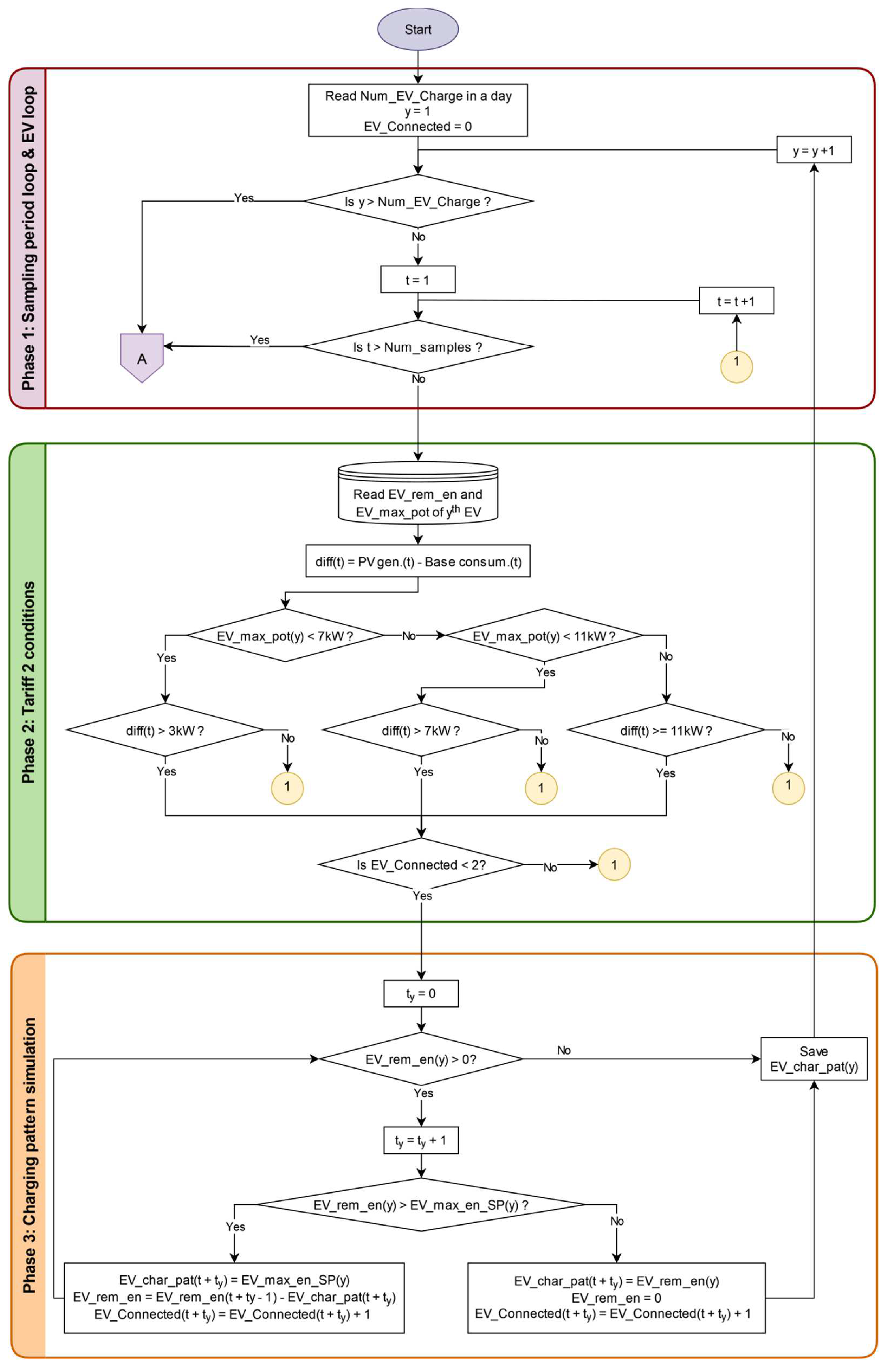
The second TS is similar to the first one. However, a more customised approach is considered. As described in
Section 2, each EV has a maximum charging power. Three power levels are mainly found: one at 3.4 kW, another one at around 7 kW, and the last one at 11 kW. In TS2, the reduced price is offered when the PV surplus exceeds one of these 3 values. Three different tariffs are published, customised to the maximum charging power of each EV. The aim is to make the most of all the time slots where there is sufficient PV surplus to charge each EV. Thus, EVs that consume less are charged when there is less surplus, and EVs that consume more are charged when there is more surplus, thereby allowing them to consume less energy from the grid.
This charging scheme is also indirect. As with TS1, the simulation of the charging patterns was processed in the recorded historical order of EV charging. In addition, once the EV connected, its charging continued at its maximum power until it was fully charged.
Figure 3 shows the flow chart that describes the simulation process of the charging for one day under the influence of TS2. Phases 1 and 3 of the flow charts are the same as those of
Figure 2. The difference between TS1 and 2 lies in the conditions under which the reduced price is offered in the second phase.
In this phase, first, the maximum charging power (EV_max_pot) of the yth EV is detected. Depending on the value of the maximum charging power of the EV, a different tariff is offered. Hence, once the maximum charging power of the EV is known, it is classified into one of these three groups: charging power (a) lower than 7 kW, (b) between 7 and 11 kW, and (c) greater than or equal to 11 kW. After classifying the yth EV within the corresponding group, the difference between the consumption and the PV production at time t (diff(t)) is calculated. If the variable diff(t) exceeds the threshold of the corresponding group, yth EV charging is carried out. For group a), for EVs with maximum charging power under 7 kW, diff(t) must exceed 3 kW. In group b), for EVs with charging power between 7 kW and 11 kW, diff(t) must exceed 7 kW. And finally, in group c), for EV maximum charging power greater or equal to 11 kW, diff(t) must exceed 11 kW. On the contrary, if the difference does not exceed the corresponding threshold, t is incremented, and the difference is recalculated and compared with the corresponding threshold for each group. Whenever diff(t) is greater than the threshold, the availability of free space at the charging point is checked. If the variable EV_Connected is less than 2, this means that there is space available, and the simulation of the EV(y) charging pattern starts.
3.4. Tariff System 3
TS3 operates as a hybrid configuration. In addition to offering reduced prices to motivate the user to switch the charging to a more convenient time, it also acts on the charging power of EVs. Therefore, it avoids consuming energy from the grid and maximises the use of PV surplus. However, in cases where there is no more PV surplus for the rest of the day, only those EVs that are still connected finish their charge by consuming energy from the grid. This process was considered to be more realistic.
The control of the EV charging power is carried out by the public charger that communicates with the EV batteries’ BMS.
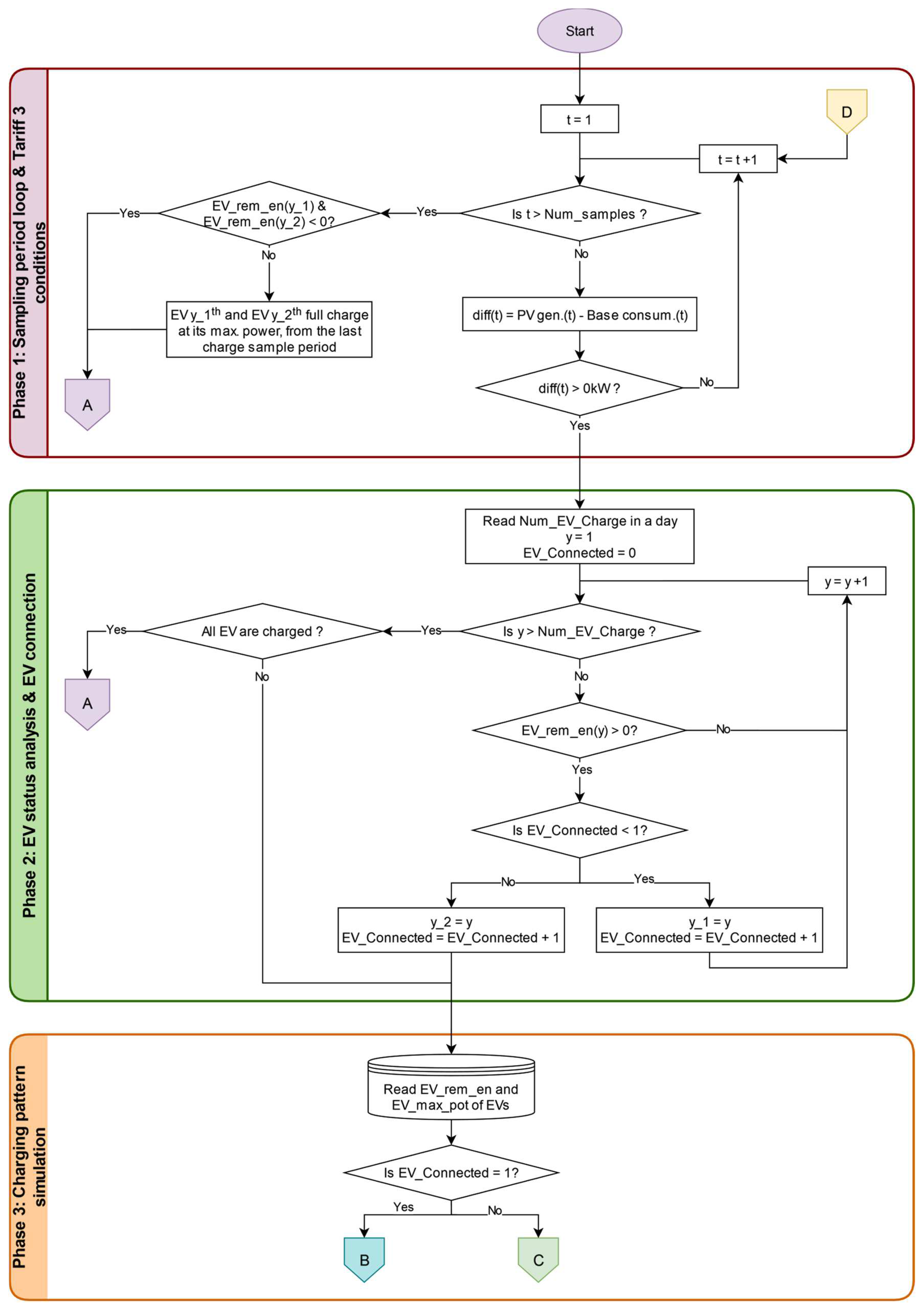
Figure 4 shows the flow chart related to TS3. The three phases are different from the diagrams in
Figure 2 and
Figure 3. This is due to the hybrid nature of the system, in which the charging power is controlled.
The initial phase is responsible for the analysis of the PV surplus for all sampling periods within a day. Starting with the first period (
t = 1), the difference between PV production and baseline consumption is calculated. If there is a surplus, i.e.,
diff(
t) > 0, the simulation for EV charging can begin. Conversely, if no surplus exists,
t is incremented, and the difference is recalculated. Finally, when
t exceeds
Num_samples (144), it means that EV charges are completed. At that point, to align with real-world scenarios, if an EV was connected during a surplus period but did not complete its charge, it continues to charge at its maximum power (
EV_max_pot), consuming electricity from the grid, starting from the last period at which it was charged. The end of
Figure 4′s flow chart is achieved when the connection point A is reached. At this point, the simulation of EV charging related to TS3 is finished.
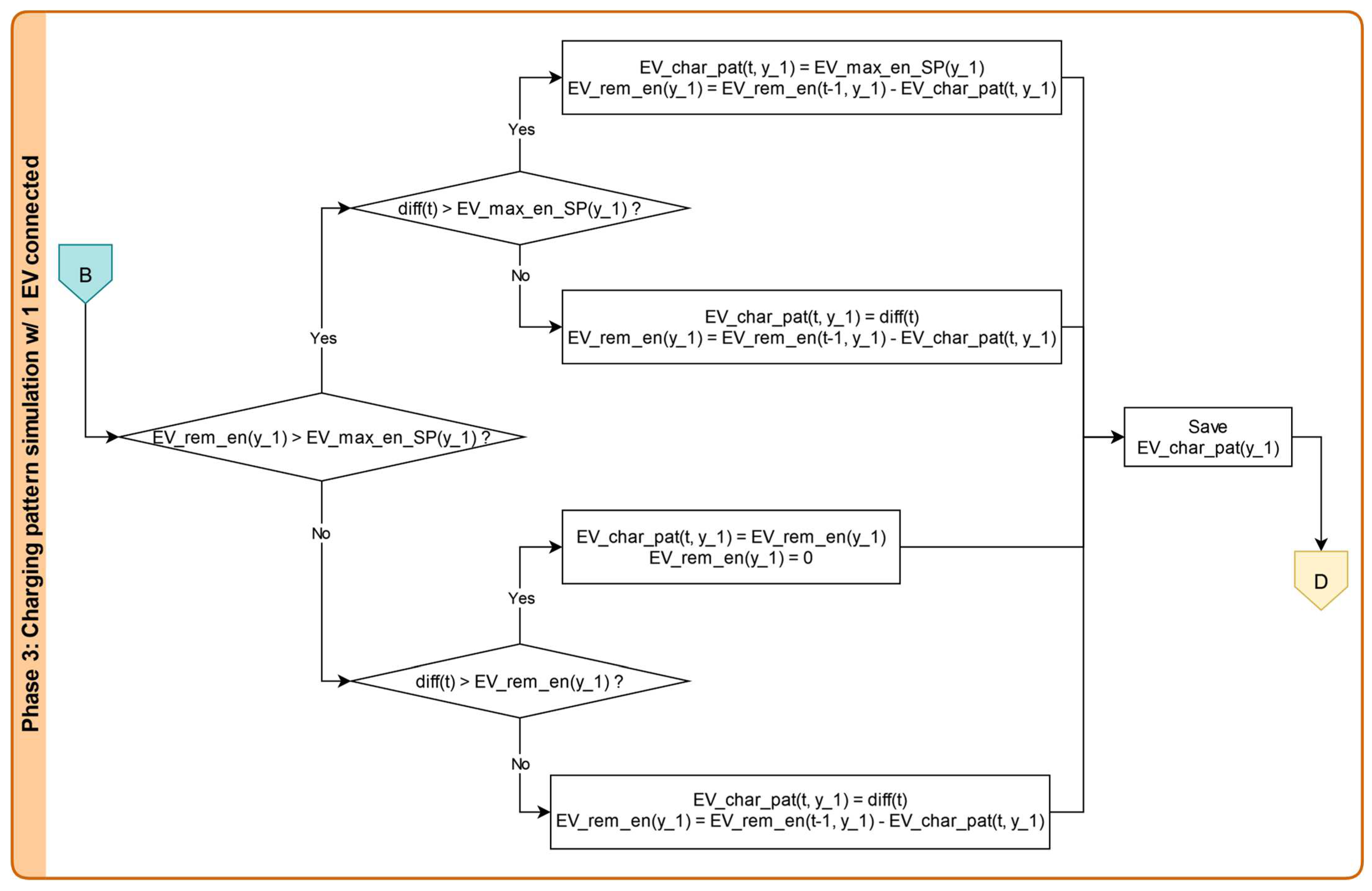
In the second phase, EVs are connected. First, EV data for the day to be simulated are read. The algorithm begins by analysing the status of the first EV (y = 1). If the yth EV is not yet charged, i.e., if EV_rem_en > 0, it is connected. On the other hand, if the yth EV is already charged, y is updated to 2 to assess the status of the next EV of the day. Before EV connection, it is verified that there is an available slot. If no EV is connected (EV_Connected < 1), the first EV connects on one connector, index y_1 obtains the value of yth EV (y_1 = y). Conversely, if EV_Connected equals 1, the second EV is connected on the last connector, and index y_2 obtains the value of the yth EV (y_2 = y), and the charging simulation begins. Finally, when y is greater than Num_EV_Charge, it is checked that all connected EVs are fully charged. If there is an EV connected, it starts being charged.
The third phase oversees the simulation of the EV charging pattern. The charging pattern of the vehicles is not the same if there is a single EV connected or two. When only one EV is connected, all the surplus of the period t is used to charge the single EV, whereas when two EVs are connected, the PV surplus is divided between the two EVs. This is why two different situations are distinguished, leading to a B connector or a C connector.
Figure 5 describes EV charging when only one EV is connected. Firstly, two possible situations are analysed: whether (
EV_rem_en) is greater than
EV_max_en_SP, or the opposite. If the
yth EV still has much energy left to complete its charge and there is enough PV energy, the charging is performed at the maximum EV power. Otherwise,
yth EV charging power varies to match the momentary surplus, i.e.,
diff(
t). This is the main property that characterises the third TS. Similarly, in this case, the
yth EV is at the end of its charge and must consume less than
EV_max_en_SP, and it is checked if there is enough PV surplus. Then, as before, in the case there is sufficient surplus, the EV is fully charged. On the other hand, if
diff(
t) is not enough to finish the charge, the EV modifies its charging power to adjust to the PV surplus. Once the charge has been completed for the sampling period
t, the simulation starts again from the first phase (connector D), analysing the situation of the next sampling period (
t + 1).
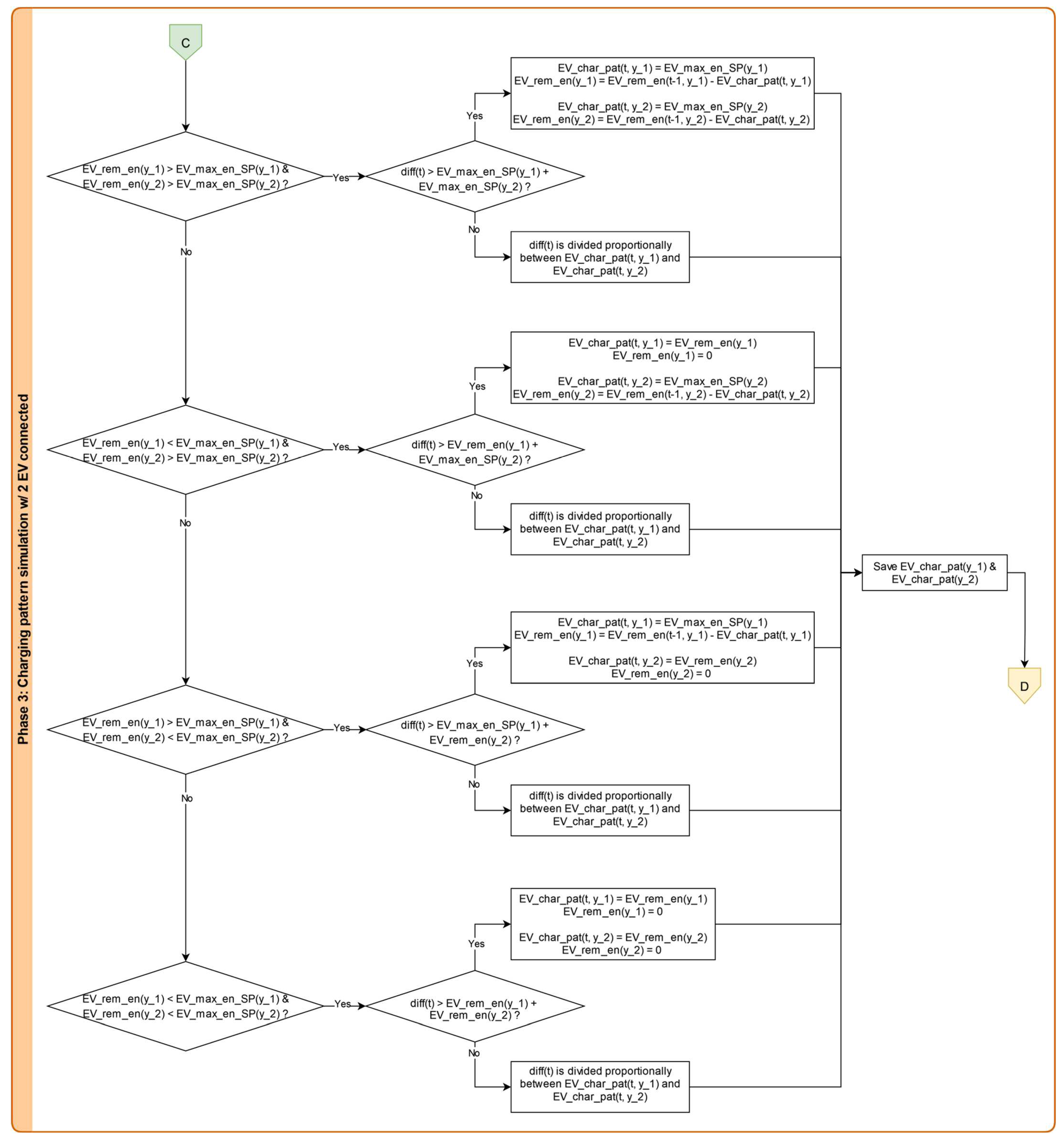
The other possible scenario is described in
Figure 6, where the flow chart for charging two EVs at the same time is presented. In this case, with two EVs, four possible situations are considered.
Both EVs still have energy remaining to be charged to their maximum power;
The EV on connector 1 (y_1) is almost charged and its remaining energy is less than EV_max_en_SP, while the EV on the second connector (y_2) can still be charged to maximum power;
In contrast to case two, the EV at connector 1 (y_1) still has a considerable amount of charge left, and the EV at connector 2 (y_2) is at the end of its charge;
Both EVs are at the end of their charge and consume less than EV_max_en_SP.
Once the situation of the two connected EVs is determined, it is analysed whether the PV surplus is sufficient to charge the EVs under the conditions determined in the previous step. If there is enough PV energy, both EVs are charged with the energy they need for each situation. On the other hand, the charging power of the EVs is modified, and the surplus is divided between the two EVs without consuming energy from the grid. Not all EVs are charged at the same power, so the amount of the surplus is considered and divided proportionally. At the end of the interval t, the flow chart starts again from the first phase until variable t is greater than Num_samples.
3.5. Charging Cost Calculation
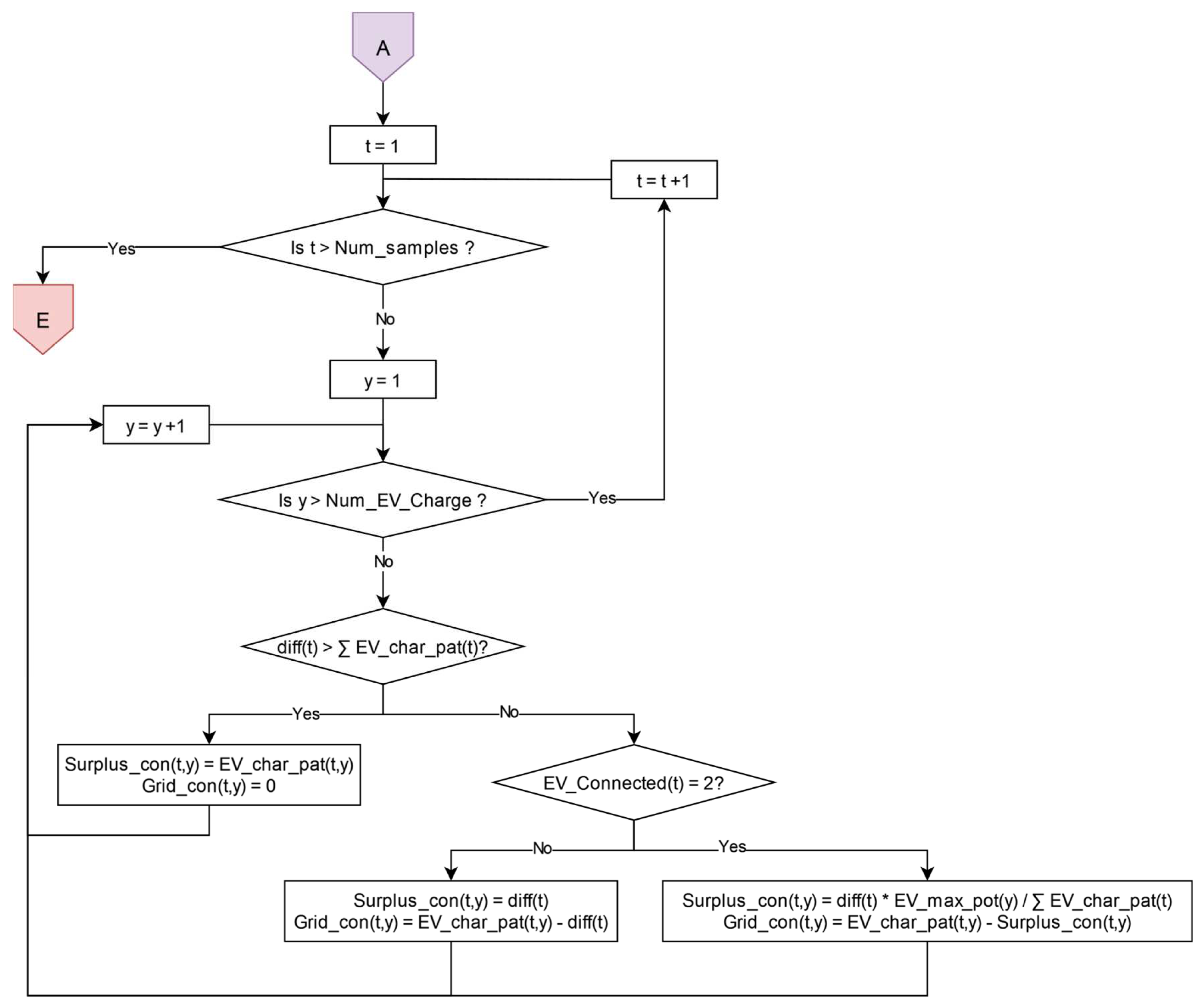
The calculation is carried out at the end of the flow charts for the three charging systems (connector A). The flow chart in
Figure 7 determines how much energy has been consumed from the grid and the PV surplus at each interval.
In each interval, the charge pattern of each EV is analysed. If the PV surplus of that sampling interval is greater than the charge of all EVs for that sampling interval, it means that the consumption corresponding to the EV charge pattern for the sampling interval t is completely consumed from the PV surplus. Otherwise, the PV surplus is divided in proportion to the maximum charging power of each EV. The remaining energy to complete the charging pattern is obtained from the grid (Grid_con).
This way, the EV charging pattern for the day is divided between the energy obtained from the PV surplus (Surplus_con) and the energy obtained from the grid (Grid_con).
Figure 7.
Division of EV consumption between PV surplus and grid. The letters A and E are connectors that link the existing flowchart to the other flowcharts above.
Figure 7.
Division of EV consumption between PV surplus and grid. The letters A and E are connectors that link the existing flowchart to the other flowcharts above.
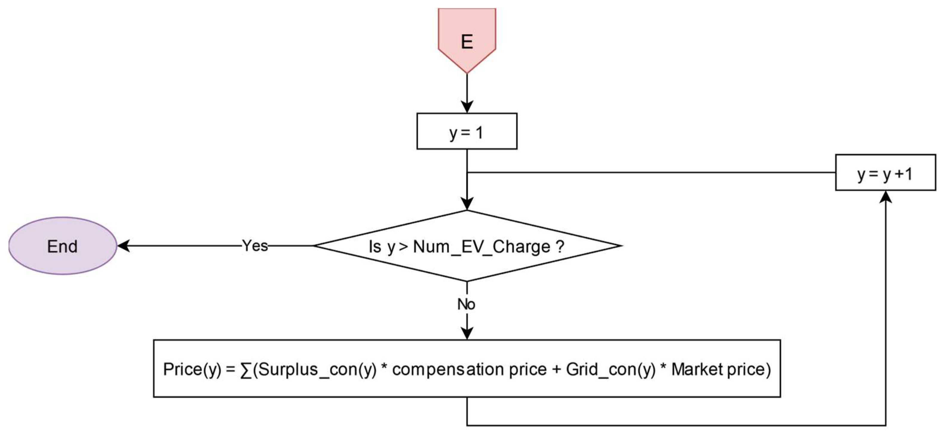
The energy consumed from the surplus is paid at the reduced price, i.e., the compensation price. Conversely, energy consumed from the grid is paid according to GoiEner’s 3.0TDVE tariff, described in
Section 3.1, as described in the flow chart in
Figure 8.
3.6. Self-Consumption Rate Calculation
Since the main objective of the three designed TSs is to maximise the consumption of locally produced energy and to decrease the consumption of the grid, the metric used to compare the different TSs is the SCR (Equation (3)).
The SCR is defined as the amount of PV energy consumed at each time step, corresponding to each hour in Spain.
where
represents the self-consumed energy in each calculation section period
k, 1 h in Spain.
represents the PV energy produced in each considered
k period.
4. Results and Discussion
The following section presents the results obtained from simulations of EV charging patterns under the influence of the three proposed TSs and their impact on the SCR.
4.1. Influence of the Three Tariff Systems for One Day in Detail
4.1.1. Day Example to Understand the Phenomenon
Firstly, 19 March 2022 is chosen as an example to observe the effect of the three proposed tariffs on the SCR.
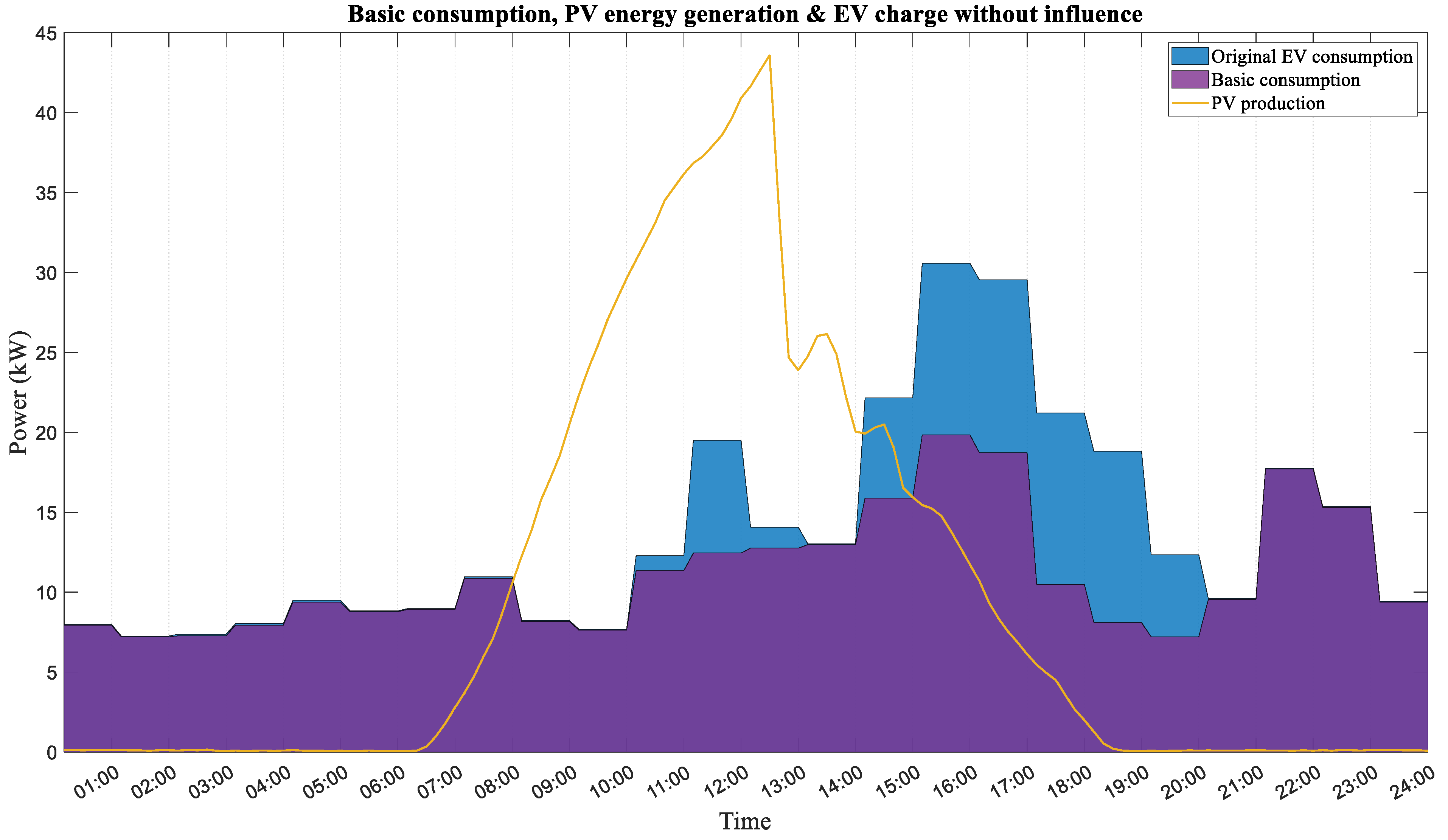
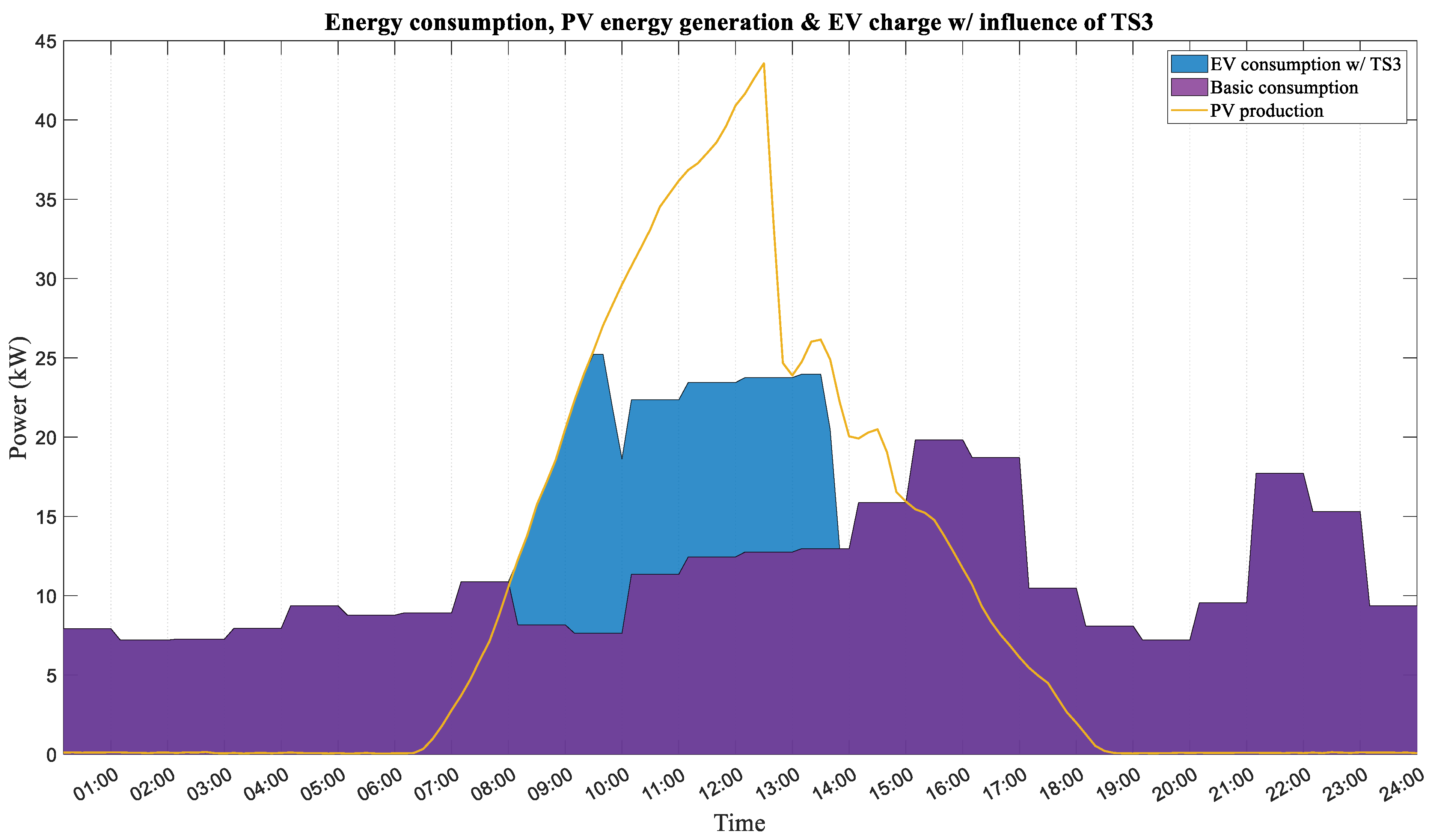
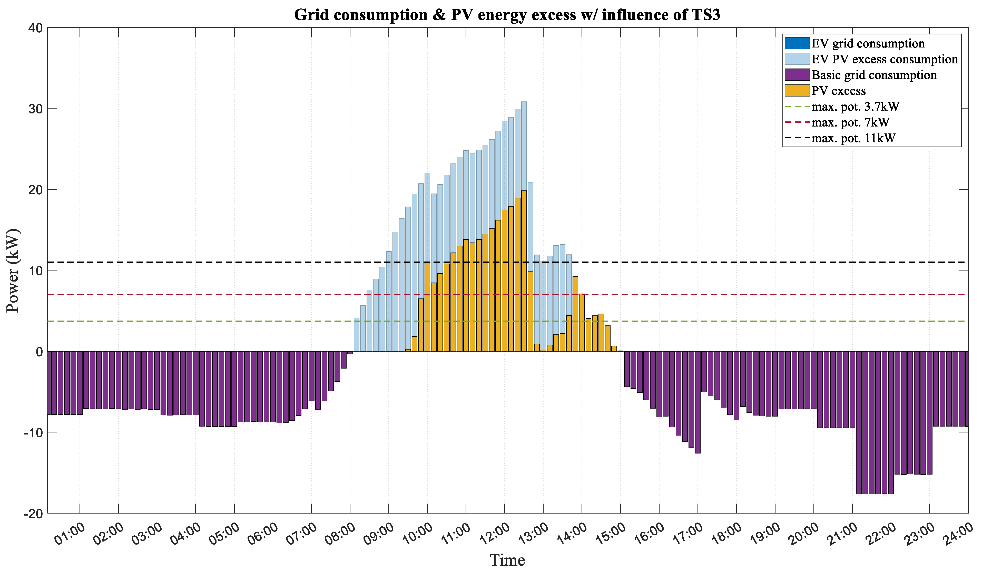
Figure 9 shows the basic consumption and the EV consumption recorded in the Charge and Parking manager. The purple area reflects the consumption of the seven points associated with the CSC. The yellow curve represents the PV production, whereas the white area refers to the unconsumed PV surplus. The blue area represents the original consumption of the EV charging registered for that day. Two EVs were charged on 19 March 2022, with 6.6 kW and 11 kW of maximum charging power.
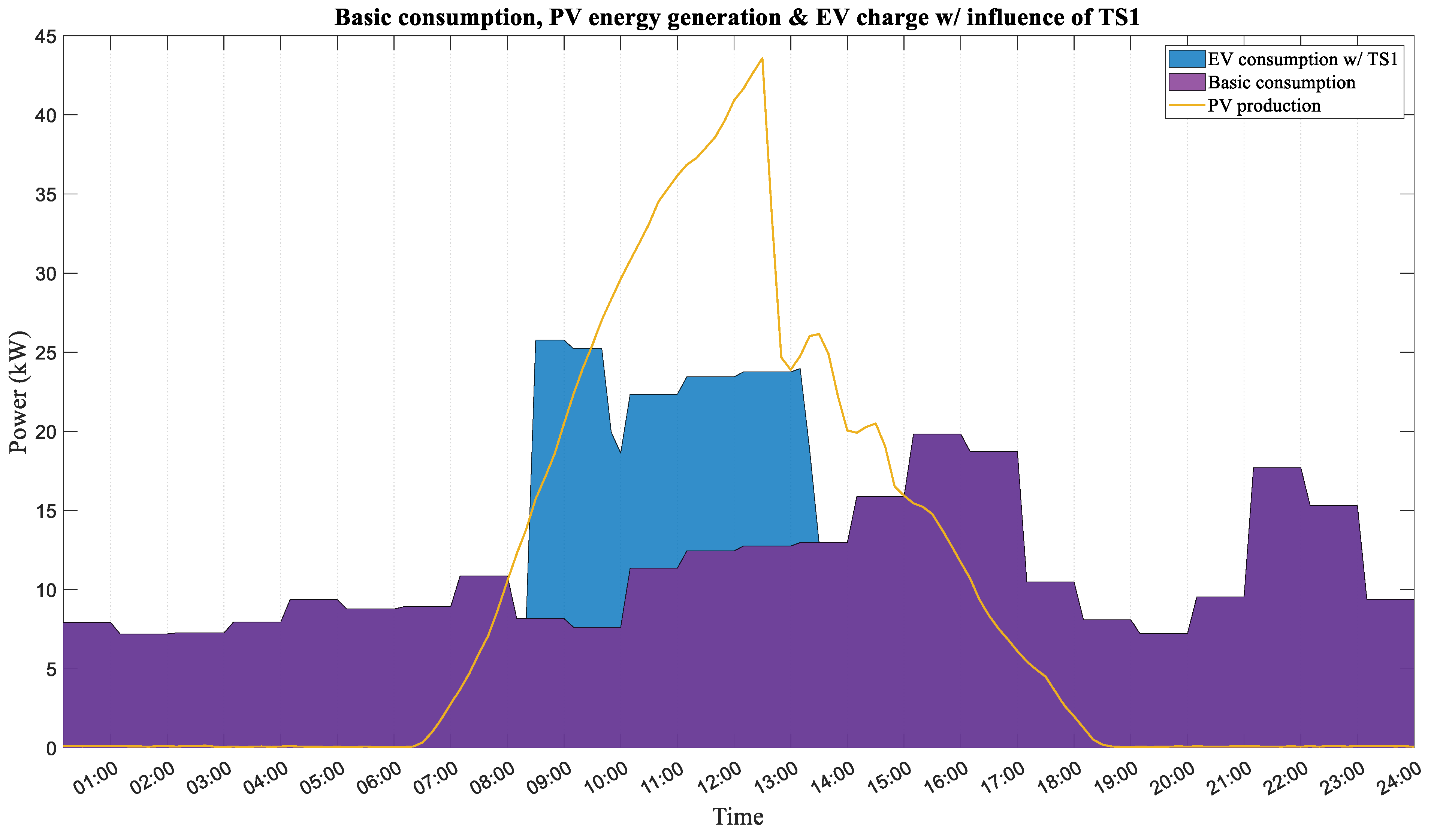
Figure 10 and
Figure 11 describe the basic consumption and EV consumption under the influence of TS1. Compared with
Figure 9, it can be observed that the charge of the second EV has been shifted to the hours when PV surpluses occur.
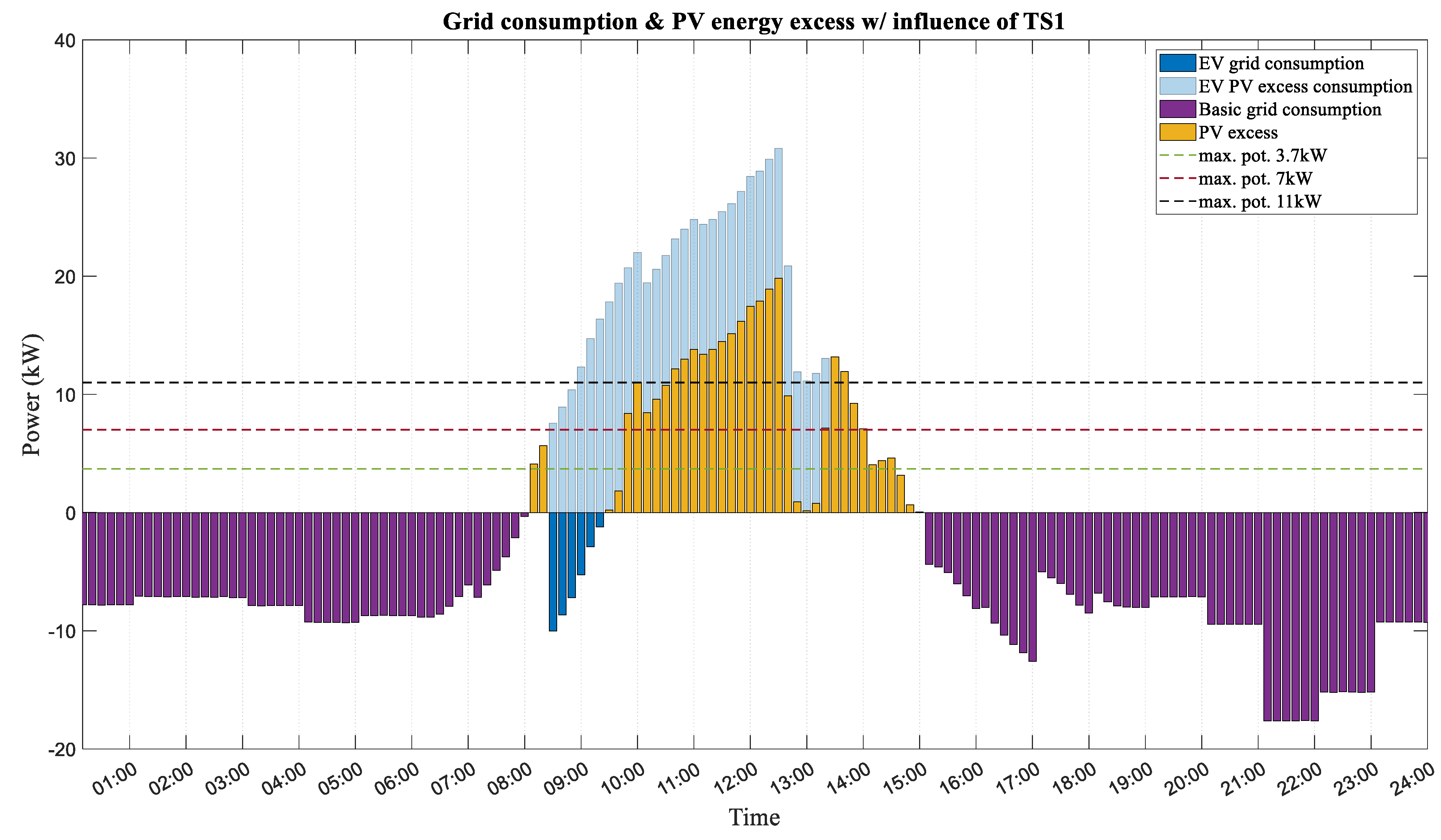
A more detailed analysis is provided in
Figure 11. Negative consumption denotes energy consumed from the grid. The light blue bars indicate consumption from PV surplus, while the dark blue ones in the negative area are the consumption from the grid. Furthermore, three horizontal lines are included, marking the threshold corresponding to 3.7 kW, 7 kW, and 11 kW. In TS1, the reduced price is offered when the PV surplus exceeds 7 kW. Therefore, the charging of both EVs is not carried out until 08:30. It should be noted that, although
Figure 11 shows that there are more PV surpluses, a part is consumed from the grid. This is due to the fact that TS1 is an indirect control where the charging power is not controlled.
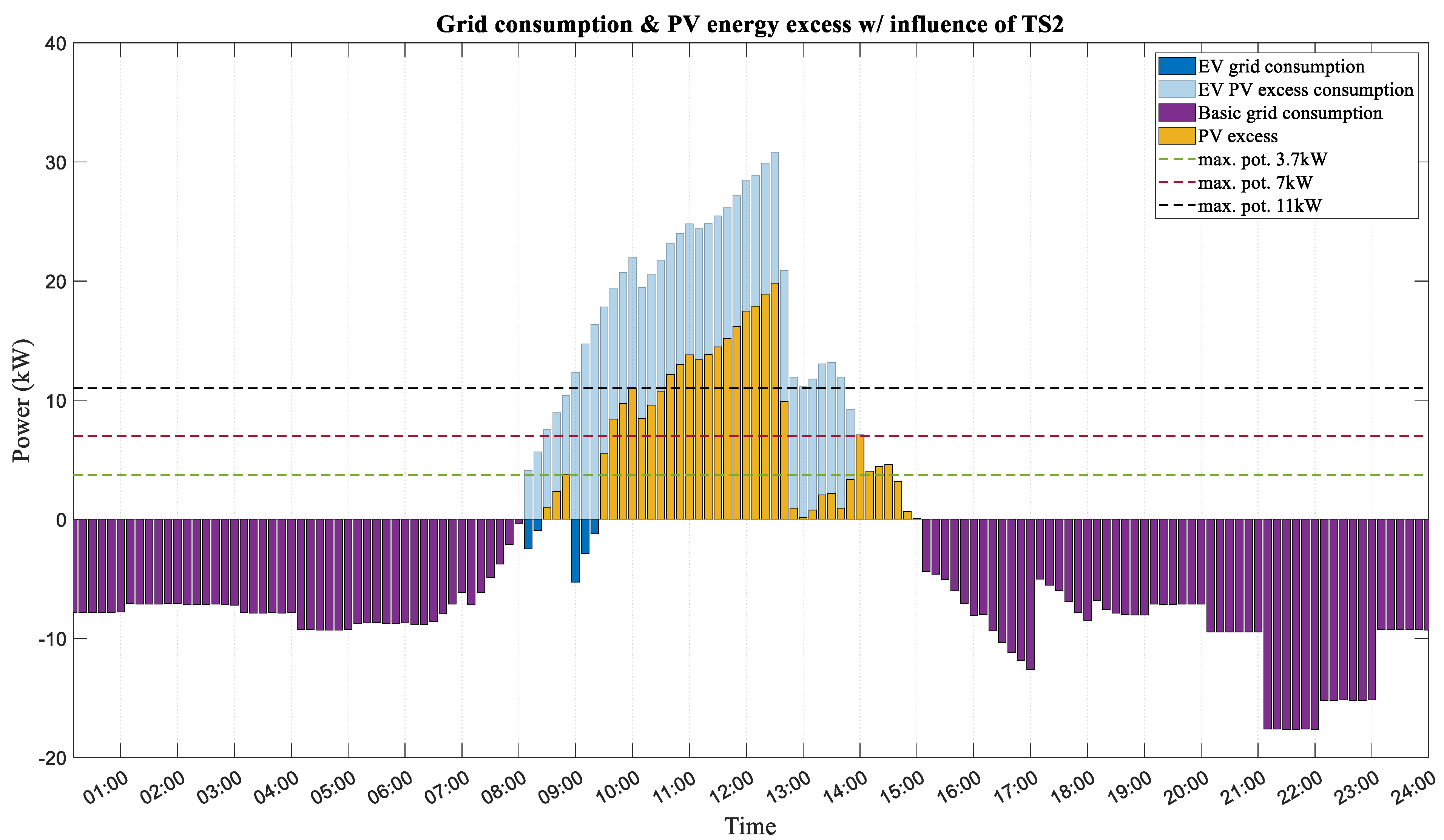
Figure 12 and
Figure 13 are related to TS2. TS2 offers a reduced price depending on the maximum charging power of each EV. In this case, the first EV with a charging power of less than 7 kW benefits from the reduced tariff when the PV surplus exceeds 3.7 kW. The second EV, with a charging power of 11 kW, benefits from the reduced tariff when the surplus exceeds 11 kW. With TS2,
Figure 12 illustrates how the blue area has expanded further into the yellow curve (PV surplus). Nonetheless, a small part is still consumed from the grid.
Figure 13 shows that by offering tariffs customised to each EV’s charging power, the charging time of each EV is better distributed depending on its power and surplus.
Finally,
Figure 14 and
Figure 15 present the consumption under the influence of TS3, where, whenever surpluses occur, the reduced charging price is offered. In addition, this system operates with direct control, modifying the charging power of the EVs. As illustrated in
Figure 14, the EV charging consumption (blue area) is perfectly aligned with the yellow curve (PV surplus), without consuming from the grid. The same result can be seen in
Figure 15, where the EVs start charging from the first instant where PV surpluses occur, and by modifying EV charging power, no electricity is consumed from the grid.
It is appropriate to mention that the simulations performed are made under the assumption that human behaviour is ideal. That is, all EV users would be willing to modify their vehicle charging schedule. However, after conducting a survey among the members of the CSC project, the opinion of the users and their likelihood to modify their charging schedule will be considered.
Finally,
Table 1 compiles the SCR values of all the cases and the cost of the EV charges. Regarding the SCR values, firstly, it should be noted that on 19 March 2022, a considerable PV surplus was recorded, reaching 30 kW. Furthermore, only two EVs were registered at the charging point that day. Considering this fact, it was clearly impossible to achieve a 100% SCR. The remaining PV surplus, i.e., that not consumed by the EV, could be consumed, at least partially, by the remaining flexible loads of the other seven consumption points of the CSC. Future work will analyse how the SCR could be further increased.
4.1.2. Different Characteristic Days Analysis
Two other days with different characteristics are analysed.
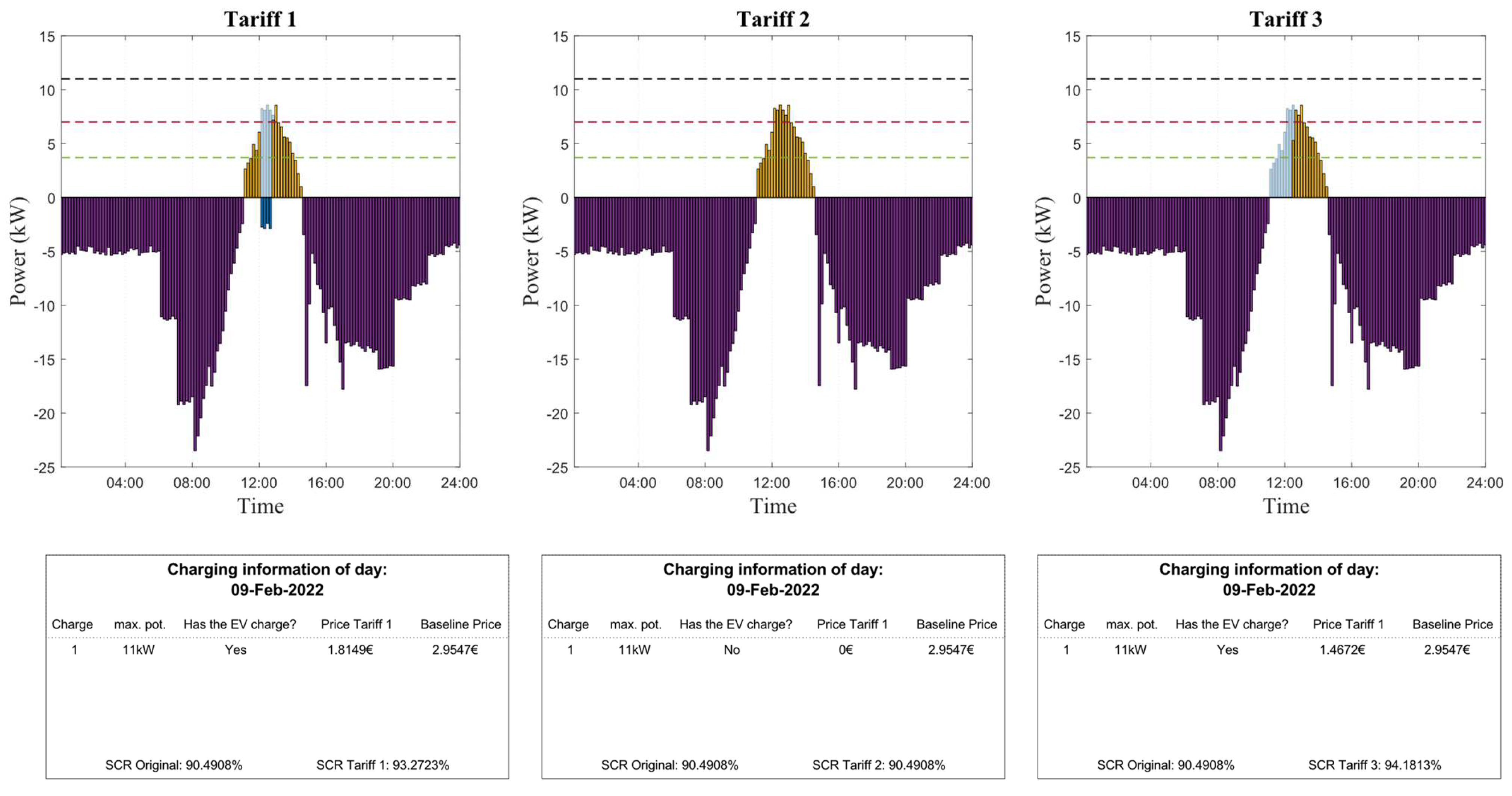
Figure 16 compiles the charging patterns under the influence of the three tariffs on 9 February 2022, where a single EV with a power of 11 kW was charged. The EV is charged with TS1 as the surplus exceeds the 7 kW threshold at some times. Regarding TS2, it is not applied to this EV since the surplus does not reach 11 kW. Finally, with TS3, the EV is charged as soon as PV surplus energy is available, without the need to consume from the grid. As far as SCR is concerned, with TS1, the SCR increases from 90.49% to 93.27%, while with TS3, it increases to 94.18%.
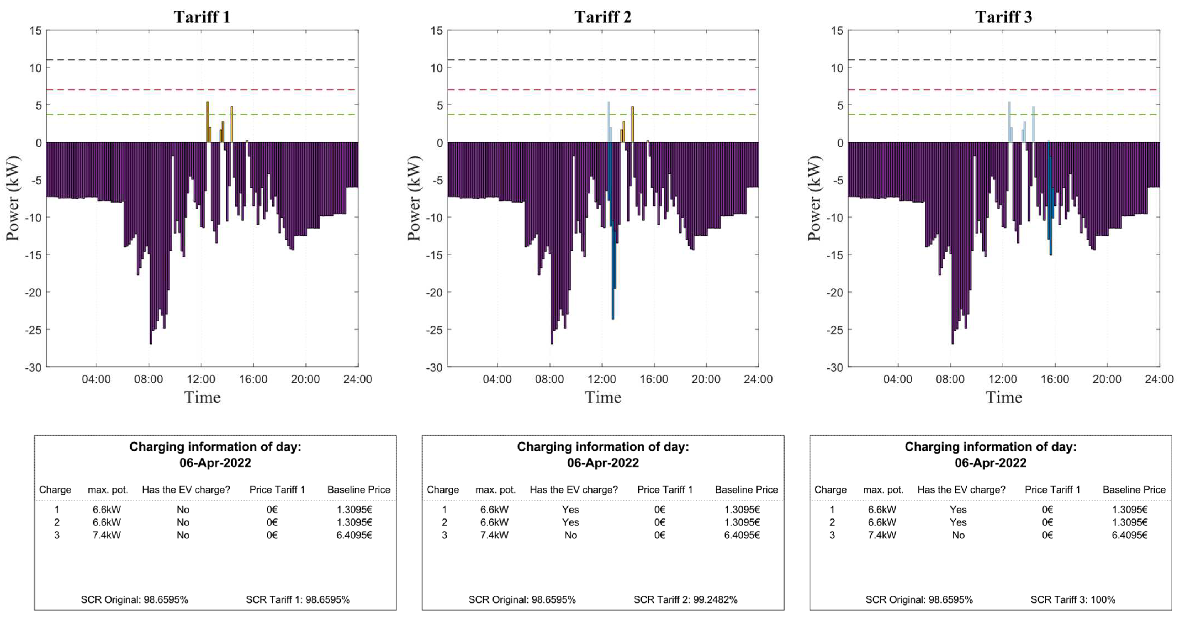
Figure 17 examines the situation for 6 April 2022, where there are almost no PV surpluses, and the basic SCR is 98.66%. That day, as the surpluses do not reach the 7 kW threshold required for TS1, this TS remains unapplied. Under TS2, a reduced price is offered to the first two EVs that have a charging power of 6.6 kW. The third EV with a power of 7.4 kW is not charged. Indeed, as in TS1, the surplus does not reach 7 kW. With TS2, the SCR increases to 99.25%. Lastly, with TS3, all surpluses are consumed, reaching a SCR of 100%.
4.2. Analysis of the Effect of the Three TSs on the SCR over One and Six Months
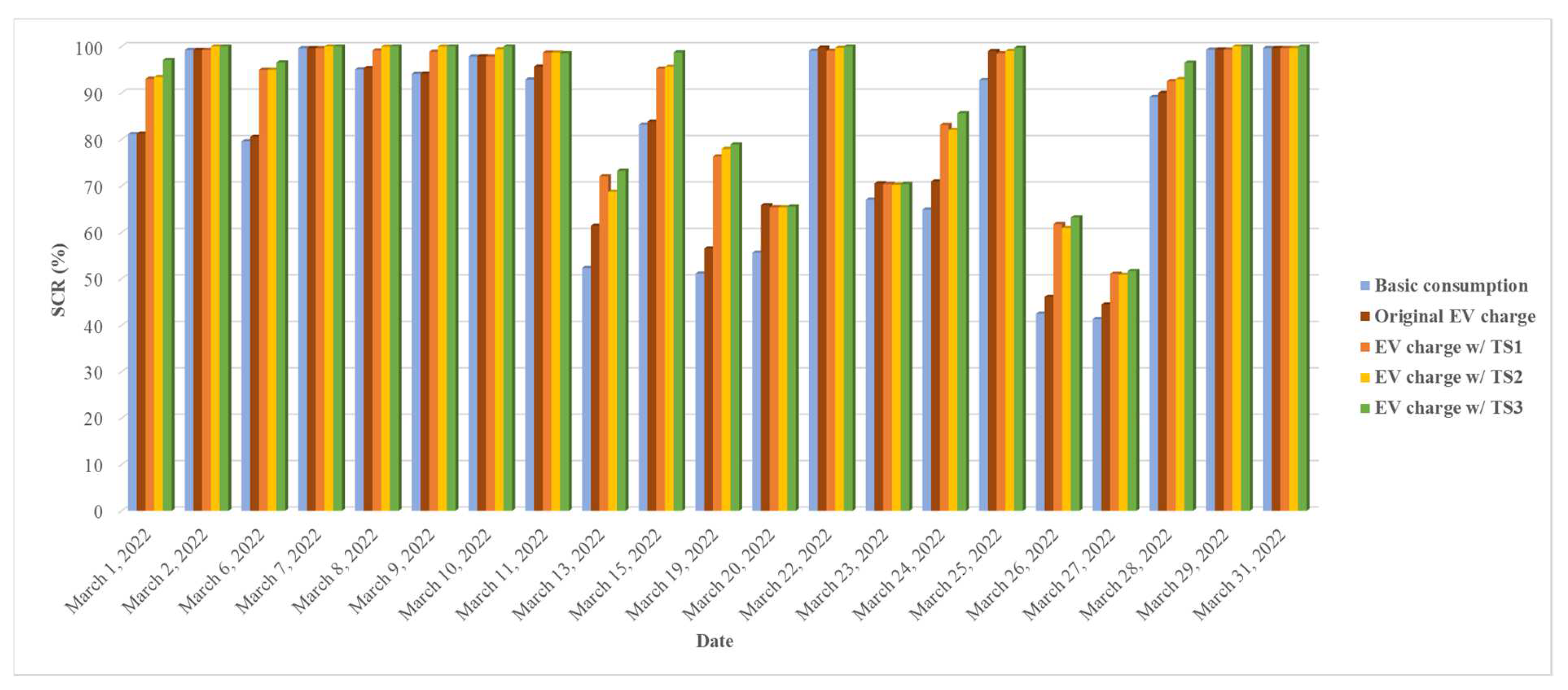
Figure 18 presents the SCR for all days where charging occurs during the month of March 2022, as long as the basic SCR is below 100% (i.e., there are PV surpluses). SCR values are depicted for the basic consumption, the original charging recorded by the Charge and Parking manager, and the three designed TSs. TS3 always obtains the highest SCR values. On the other hand, most of the time, TS2 obtains higher SCRs than TS1. In addition, it is noticeable that on days with a high basic SCR, the increase in SCR is not as significant as on the other days.
Table 2 presents the average SCR values for each month and the overall average for all simulated days over the 6 months. The overall average basic SCR is 83.82%. The SCR obtained with the original charge of the EVs is 86.54%. The average SCR stands at 90.86% with TS1, 91.04% with TS2, and 93.09% with TS3. It can be concluded that these TSs clearly show an improvement in self-consumption, achieving an increase in SCR of 8.8% when applying TS3, for instance.
4.3. Comparison of the SCR Increase in the Three TSs with the Original Charge
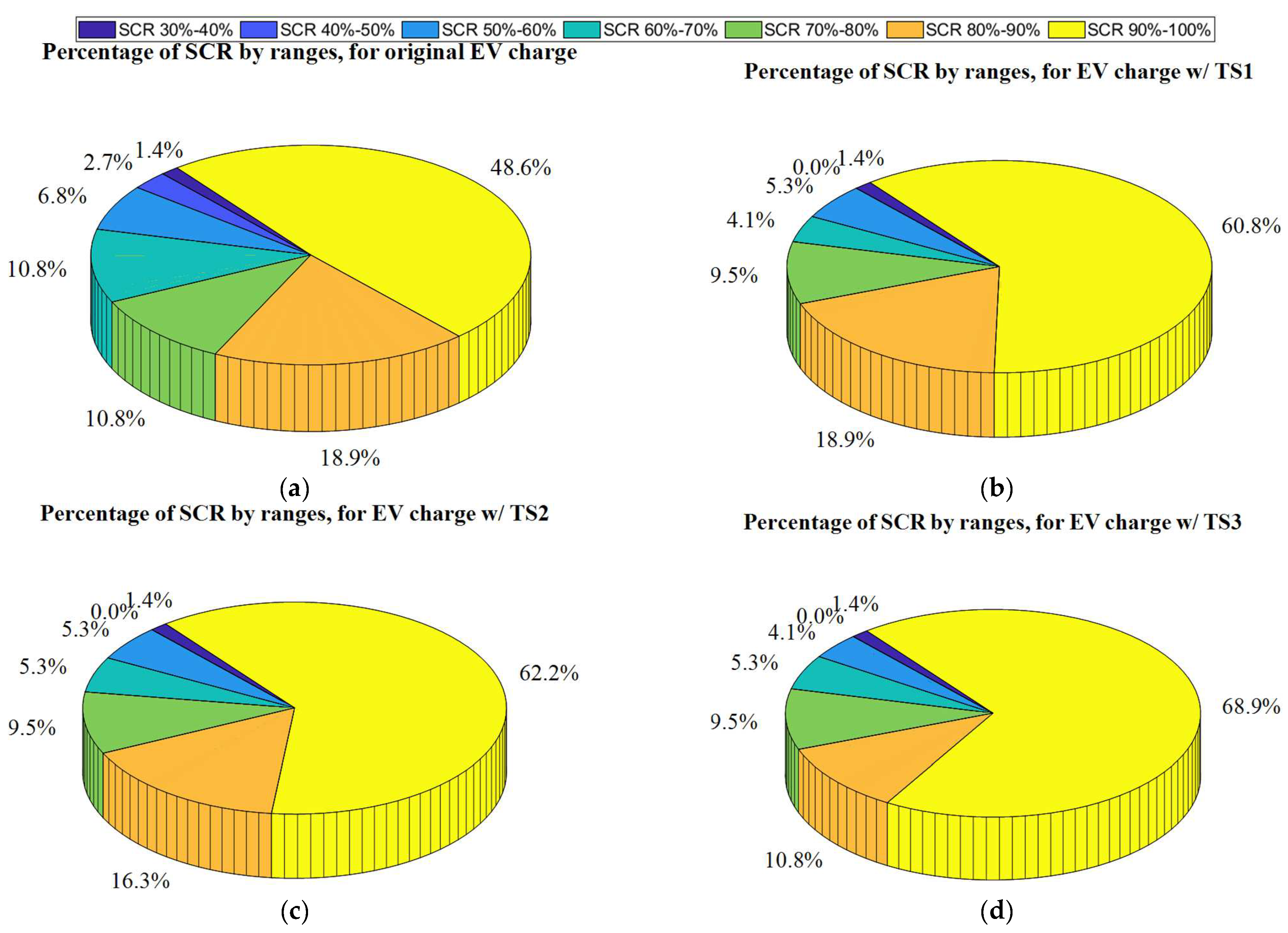
Figure 19 presents four pie charts divided into ranges based on the SCR values. For instance, the yellow range shows all days when the SCR is between 90% and 100%.
Figure 19a displays SCR values related to the original charge registered by the Charge and Parking manager. Results obtained with TS1, 2, and 3 are shown in
Figure 19b–d, respectively. It is noticeable that in 21.7% of the days, SCR values below 70% are obtained with uncontrolled charging. Conversely, with TS1, these values are reduced to 10.8%, 12% with TS2, and 10.8% with TS3. On the other hand, when examining higher SCR, without TS, a SCR higher than 90% is obtained only 48.6% of the time, while these data increase to 60.8% with TS1, 62.2% with TS2, and 68.9% with TS3.
4.4. Analysis of the Economic Savings of the Three TS
Table 3 compiles the average percentage savings for each month from the EV user’s point of view. With TS3, more energy is consumed from PV surplus and less from the grid. Therefore, it is also the TS that provides the most economic savings, achieving savings of 32%. Finally, the values of the global average over the six months indicate that both TS1 and TS2 achieve the same savings of 22%. As for TS3, an average of 25% savings is obtained for each EV charge.
5. Conclusions and Future Works
The research study presented in this paper analyses three TSs for EV charging based on PV surplus within a CSC project. Contrary to most articles found in the scientific literature, the main objective of this work is to increase the SCR rather than to increase the economic benefits of a charging station owner. In addition to the increase in the SCR, EV users also benefit from a reduction in the charging cost. As three different tariffs are designed and analysed, stakeholders can assess which case suits them best, besides having easy replicability.
Overall, the behaviour of the TSs can be divided into two cases: when PV surpluses are low and when they are high. When they are low, there are often scenarios where TS1 and TS2 are not applied, as the surpluses do not reach the set threshold. TS3 is always offered. However, it is usually necessary to consume from the grid to complete the charging of the EVs. In these cases, the SCR is usually very high, reaching 100%. Regarding days where there is a significant amount of surplus, generally, all three TSs are offered. With a large surplus of PV, the SCR tends to be lower, but the increase in the SCR thanks to the TS is highlighted.
As for which TS is the best, all of them have their advantages and disadvantages. TS1 is the simplest to implement. Additionally, if the surplus exceeds the 7 kW threshold, all EVs are charged. As a drawback, TS1 may lead to underutilisation of PV surplus. Considering the 6-month simulations, TS1 results in a 6.2% increase in SCR compared to the original charge, while the cost of EV charge is reduced by 22%.
Concerning TS2, its main advantage lies in its significant potential on days with substantial PV surplus. However, if there are no high surplus levels, it could result in not offering the tariff to all EVs. Overall, with TS2, the SCR increase is 6.4%, and the EV charging cost is 22% lower.
Finally, TS3 proves to be the most beneficial system regarding the SCR and the economic savings of the users, with a SCR increase of 8.8% and a reduction of the cost of 25%. Its advantages lie in offering a reduced price regardless of surplus levels and controlling the charging power, thereby taking advantage of all the potential for self-consumption. On the other hand, its implementation complexity and related costs stand as a disadvantage.
It is important to note that direct control of EV charging is not always possible, especially when charging points are public. Therefore, although it has been shown that direct control leads to higher SCR increases, it is also essential to analyse ways in which higher SCR can be achieved through indirect control of EV charging. In addition, indirect controls are less costly to implement.
This study is carried out as part of a CSC project, involving eight consumption points and PV production. To conduct the calculations presented in this article, historical recorded data were used. However, in the future, the real-time EMS will use predictions of both PV consumption and production to calculate the PV surplus.
Regarding other future studies, different actions are planned. On the one hand, it is important to better represent the uncertainty of human behaviour. For this purpose, a survey of CSC members conducted by the retailer will be considered. These members will be asked about their willingness to change the EV charging time. Additionally, an analysis of the scientific literature will be carried out to determine how EV users react to charging tariffs. According to the results of these studies, probability factors that depend on the level of change in the charging time will be considered in the simulation. Finally, the confidence interval of the PV production and the consumption predictions will be considered.


