Abstract
Setting solar photovoltaic capacity targets and implementing supportive policies is a widespread strategy among nations aiming to achieve decarbonisation goals. However, policy implementation without a thorough understanding of the intricate relationship between social, economic, and land-use factors and solar photovoltaic deployment can lead to unintended consequences, including over- or underdeployment and failure to reach targets. To address this challenge, an investigation was conducted into the relationship between 36 factors and solar photovoltaic deployment across 143 countries from 2001 to 2020 using correlation analysis and principal component analysis. From these factors, five key variables were identified that collectively explain 79% of the year-to-year variation in photovoltaic capacity. Using these variables, a neural network model was constructed, enabling the estimation of capacity additions by country with an error of less than 10%. Additionally, a solar photovoltaic deployment index was developed, serving as a benchmark for comparing a country’s actual historical photovoltaic deployment to similar nations. Furthermore, the model’s utility in evaluating the impact of solar photovoltaic policies was explored. Through three distinct use cases—forecasting solar photovoltaic capacity additions, developing a solar photovoltaic deployment index, and assessing the impact of solar photovoltaic policies—the model emerges as a potentially powerful tool for governments and policy makers to assess solar photovoltaic deployment effectively and formulate strategies to promote sustainable solar energy growth.
1. Introduction
Solar photovoltaic (PV) electricity is now, on average, cheaper than fossil fuel electricity [1], and one of the cheapest sources of power production [2]. Consequently, solar PV contributes substantially to the decarbonisation strategies of many countries. For example, China aims to increase the capacity of solar and wind to over 1200 GW by 2030 [3]. Japan targets 108 GW of installed solar capacity by 2030, equivalent to 15% of its total power generation [4]. EU countries Italy, Germany, and Spain are aiming for 52 GW [5], 215 GW [6], and 37 GW [7] of solar capacity by 2030. The United Kingdom’s target is 7% of electricity from solar PV by 2030 [8], and South Africa’s target is 8 GW of solar PV, which would account for 11% of total installed capacity [9].
These capacity targets are often backed up by a range of policies to support investment in solar power production. Historically and presently, these include feed-in tariffs, where system owners are paid to export power to the grid (e.g., China, Japan, and Vietnam [8]); net metering, which compensates system owners for surplus electricity fed into the grid [10] (e.g., Botswana, Zimbabwe, Saudi Arabia, and Belgium [1,8]); utility quota obligations or renewable portfolio standards, which require a minimum percentage of generation to be provided by renewable energy of which a portion is solar PV [1] (e.g., Australia, Sweden, and the United Kingdom [8]); and tradeable renewable energy certificates (RECs), which are awarded per MWh and can be bought or sold separately from the electricity [11]. Other policy options include a reduction in tax associated with energy (e.g., Finland, France, Germany, Italy, Spain, and Japan [8]), direct investment or production tax credits to encourage businesses to develop and operate solar energy projects (e.g., Germany, Greece, Italy, Spain, and the United States [8]), and public investment loans, grants, capital subsidies or rebates, and auctions or tenders.
Implementing these kinds of policies without prior understanding of the complex interactions of geographic factors (e.g., sociological, economic, land-use, climatic, and technological) involved in PV deployment can lead to unintended consequences such as overdeployment or failure to meet the targets. Spain’s experience in 2008 exemplifies this, where rapid growth in solar PV deployment, driven by new feed-in tariffs, strained the electricity grid and necessitated sudden policy adjustments to curb costs [12]. This eventually led to market collapse in the following years. On the other hand, India, despite implementing various supportive measures such as feed-in tariffs, obligation certificates, and tax reductions, fell short of its ambitious 100 GW target by 2022, achieving only 54 GW [13,14]. Furthermore, evaluating a country’s progress in solar PV deployment based on its self-defined targets may not accurately reflect the actual deployment compared to realistic expectations, as it fails to account for the complex interplay between PV deployment and geographical factors.
The development of models that can explain the importance and interactions of the different adoption factors could be very valuable in the refinement of policies to support solar PV and its integration into the wider electricity system within a country. Such models could be used to forecast solar PV capacity in order to support network planning, and they could help with the early identification of over- or underdeployment by providing a benchmark in terms of what might be expected in terms of a comparison with countries further ahead in the deployment curve.
The aim of this study is to investigate the factors influencing country-level historical solar PV deployment, culminating in the construction of a comprehensive global model capable of estimating total PV capacity additions for any country. This model will serve multiple purposes: Firstly, as a forecasting tool for PV capacity, facilitating effective planning and generation monitoring. Secondly, as a benchmarking mechanism, allowing for comparisons with similar countries. Lastly, as an evaluative instrument for policy assessment, by comparing estimated outcomes against actual developments.
2. Literature Review
To construct a comprehensive global model, it is imperative to examine the factors influencing deployment and integrate them into our framework. To the best of our knowledge, there have not been any studies that investigate the relationship between geographic factors and solar PV deployment on a global scale. However, there are studies that investigate the relationship between these factors on household, subregional (i.e., census areas of approximately 1000–8000 people depending on country [15,16]), regional (i.e., state/county/village), and country level.
On a household level, Jan et al. [17] identified key factors for explaining solar PV adoption in northwest Pakistan, which are income, cost of energy consumption, education level, information about the solar PV market, and source of awareness about solar PV systems. They explain 38% of the variation in adoption. Letchford et al. [18] performed a sensitivity analysis using multiple methods to determine which features were important predictors of solar PV adoption in the San Diego region, US. Property size, whether the owner lived on the property, national unemployment rate, income, cost of electricity, and peer effect are all key factors that explain 33% of the variation in adoption. Aklin et al. [19] investigated solar PV adoption at the household level in rural India and found that households that are wealthy and have access to banking are more likely to use solar power.
Graziano and Gillingham [20] studied the influence of multiple factors on PV adoption in Connecticut, US, and showed that the influence of neighbours, the built environment (housing density and share of renters), and policy have a strong relationship with PV adoption compared to social, economic, and political factors. Peralta et al. [21] characterised the spatio-temporal adoption patterns of domestic solar PVs in Birmingham, UK, and found that income, electricity usage, and average household size are the best predictors of solar PV adoption.
Yu et al. [22] identified key social and economic factors correlating with solar deployment density in the US, which are solar radiation, population density, annual household income, Gini index, and education level. The Department of Energy and Climate Change [15] analysed factors that play a role in the deployment of PVs under a feed-in tariff scheme in England, UK, and found that electricity consumption, gas consumption, gas coverage, age of population, index of multiple deprivation and its various domains, dwelling stock by tenure and type, urban or rural classification, council tax band, and fuel poverty are all key in explaining solar PV deployment.
McEachern and Hanson [23] studied the adoption of solar PVs across 120 villages in Sri Lanka and found that solar PV adoption is driven by expectations of whether the government will connect the villages to the electricity grid, as well as tolerance for nonconformist behaviour. Aklin et al. [19] investigated factors that determine solar adoption at the village level in rural India and showed that remote, large, and poor villages with high levels of solar radiation adopt solar technology as a replacement for grid electricity. Mayer et al. [24] analysed the socioeconomic factors correlating with PV system adoption in 53 counties in the state of North Rhine Westphalia, Germany, and found that gross value added by agriculture was highly correlated with PV adoption with a Pearson correlation coefficient of +0.75, while unemployment rate and population density were moderately correlated with PV adoption at −0.61 and −0.64, respectively. Liu et al. [25] investigated the correlation between social and economic factors and the installed capacity of solar PV in China and showed that GDP, final consumer expenditure, industrial added value, and solar energy generation and consumption are strongly correlated with PV capacity.
When considering quantitative models that can forecast PV capacity additions, there are very few models. The World Energy Model (WEM) initially forecasts total capacity additions, irrespective of technology, driven by demand. Subsequently, the share of solar PV capacity additions is determined according to the regional value-adjusted levelised cost of electricity [26]. However, this method of estimating the required capacity and subsequently deriving the share of solar PV capacity introduces compounding errors. Historically, the International Energy Agency, the US Energy Information Agency, Bloomberg New Energy Finance, Photon, and Greenpeace all underestimated PV capacity additions [27].
The International Renewable Energy Agency (IRENA) projects global solar PV capacity additions based on current and planned policies and targets of countries, as well as the trajectory of the global energy system aimed at limiting the rise in global temperatures to well below 2 degrees Celsius above preindustrial levels [28]. However, these projections are susceptible to errors due to several factors. Firstly, the capacity targets set by countries are not always met, leading to discrepancies between projected and actual outcomes. Secondly, the emphasis on global temperature objectives does not fully account for the diverse geographic factors within each country, which can significantly influence the deployment of solar PV capacity.
In academia, Yu et al. [22] developed a machine learning model that uses socioeconomic and environmental factors to accurately predict solar PV deployment density in US subregions. The model is a two-stage model that uses a random forest classifier to determine whether any solar PV systems exist in a census area and a random forest regressor to estimate the solar deployment density. The model achieved a cross-validation of 0.72, but it uses a large number of US-specific input features (>90), which makes it difficult to replicate in another country. In addition, it only takes into account residential PV systems.
Liu et al. [25] built a bidirectional long short-term memory neural network model to forecast China’s solar PV installed capacity and achieved a mean absolute percentage error (MAPE) of 6%. A mean impact value analysis was performed to determine the contribution of each factor in the model. Solar power generation, solar power consumption, gross domestic product, final consumer expenditure, and industrial added value contributed 26%, 27%, 17%, 15%, and 14%, respectively. This model uses a small number of input features, but it relies on solar generation and consumption data, which are not available for most countries.
Remote sensing-based methods have emerged as a promising solution for acquiring information on PV installations. These techniques use overhead imagery and deep neural networks to detect and map solar PV capacity using computer vision. For instance, Ravishankar et al. [29] devised a deep learning framework to estimate the global capacity of solar farms from high-resolution satellite imagery, achieving an average error rate of 4.5% when validated against publicly available data; while this method effectively detects large-scale solar installations, it can be computationally expensive. Detecting small-scale solar PV installations is more complicated as it necessitates high-resolution imagery to maintain model performance [30,31]. Recent advancements, such as the development of electric-dipole gated phototransistors, offer high-performance imaging capabilities with reduced power consumption, promising improved machine vision imaging models in the future [32].
These studies investigated factors associated with PV adoption, which were used as a guide for selecting factors in the present study. The focus extends to total national capacity additions, regardless of type (residential, commercial, utility scale). Existing global models estimate capacity based on national targets, leading to inaccuracies. Furthermore, national or subregional capacity models often rely on data unavailable in many countries, and while remote sensing-based vision models offer a promising solution for acquiring information on PV installations, their reliance on high-resolution imagery can be impractical in regions where such data are scarce or expensive to obtain.
To overcome these difficulties and develop a common framework for analysis of national PV capacity across many countries, an attempt is made to build a generic model that relies on open source global databases. Fortunately, global databases of historical data are available. Weather data are available as a record of meteorological variables and include irradiance [33], the key determinant of solar PV production. The International Energy Agency (IEA) and Euro-Mediterranean Center on Climate Change (CMCC) provide records of averaged weather parameters specific to each country, such as temperature, daylight hours, snowfall, cloud coverage, and precipitation [34]. The World Bank documents country-level demographics such as population, average age, level of education, employment, and national economics such as gross domestic product and gross national income [35]. The World Bank also documents land use such as urban, rural, and agricultural. The International Renewable Energy Agency (IRENA) reports country-level solar PV capacity additions on an annual basis [36]. The Energy Information Administration (EIA) tracks annual electricity consumption and generation by source such as nuclear, fossil fuels, and renewables [37], and the Renewable Energy Policy Network for the 21st Century (REN21) documents national and subnational solar PV policies [1].
3. Methodology
3.1. Determining Key Features Associated with Global Solar PV Capacity Additions
To build a global model, potential geographic features with global coverage needed to be determined. Table 1 shows the investigation conducted into the relationship between 36 climatic, social, economic, and land-use features and solar PV capacity additions. The Pearson’s correlation coefficient was calculated for each factor in relation to solar PV capacity additions. The coefficient of determination () was determined by fitting linear regression models between each feature and solar PV capacity additions. Finally, principal component analysis (PCA) was applied to measure the similarity between features. Similar features were clustered together, and the percentage of variation explained in a cluster by each of its members was calculated. The total percentage of feature data variation explained by each cluster was also calculated. The data in Table 1 cover 143 countries around the world, span the years 2001 to 2020, and have a temporal resolution of one year.

Table 1.
Features considered for modelling solar photovoltaic capacity additions. The definition, category, and availability of the data are shown. The correlation and coefficient of determination () with solar photovoltaic capacity additions are calculated. Principal component analysis (PCA) is performed, and similar features are clustered together. Finally, the literature that used the same or similar features is linked.
PCA results in Table 1 show that the first cluster’s members are mostly economic features. It explained 22.4% of the variation in the feature data and was highly correlated with PV capacity additions. When fitting the cluster features in a linear model, it explained 76.9% of the variation in PV capacity, as shown in Table A2. The most important features in the first cluster were last year’s PV cumulative capacity, electricity net generation, and consumption.
The second cluster comprised mostly climate features and explained 11.6% of the variation in the feature data. When the cluster features were fitted into a linear model, they accounted for 21.1% of the variation in PV capacity, as shown in Table A2. However, the number of data points for this cluster was less than 1% of the dataset, a limitation attributed to the methodology of fitting multiple features simultaneously. Specifically, when fitting more than one feature, rows with missing data points for any feature were excluded from the analysis. As shown in Table 1, features from this cluster were not correlated with PV capacity additions and did not explain the variation in PV capacity.
The third cluster consisted mainly of land area features and explained 10.3% of the variation in the feature data. When the cluster features were fitted into a linear model, they accounted for 22.2% of the variation in PV capacity, as shown in Table A2. The most significant feature in this cluster was agricultural land area.
The fourth cluster consisted of social features and explained 18.2% of the variation in the feature data. When the cluster features were fitted into a linear model, they accounted for 46.3% of the variation in PV capacity, as shown in Table A2. The most significant feature in this cluster was tertiary education. The remaining clusters explained less than 10% of the variation in the feature data.
Economic factors played the largest role in explaining the variation in solar PV deployment, followed by social factors. Land use played an important role but was less significant compared to economic and social factors. When it came to explaining the variation in the feature data, economic and social factors contributed equally, while land-use factors contributed about half as much as social or economic factors.
The Pearson’s correlation coefficient and the coefficient of determination () in Table 1 show that climate features did not play a significant role in the additions of solar PV capacity on a global scale. This was not the case on smaller scales such as regional, subregional, and household levels, where solar irradiance was a key factor [19,22].
Tertiary education was highly correlated with solar PV capacity additions (0.8) and explained 60% of the variation on a global scale, which was also the case on subregional [22] and household levels [17]. It was the most significant social feature on a global scale. This may have been because it acted as an indicator of the economy and population count in addition to education. Population count, primary and secondary education, labour force, and total unemployment were moderately correlated with PV capacity additions and explained between 10% and 30% of the variation.
The previous year’s cumulative PV capacity, economic value added by agriculture, forestry, fishing, manufacturing, industry, electricity net consumption and generation, and fossil fuel electricity net generation were highly correlated with added PV capacity and explained a high percentage of the variation (between 50% and 80%). They played the largest role in explaining solar PV deployment on a global scale. Gross domestic product (GDP) and gross national income (GNI) were moderately correlated with added PV capacity. This was not the case on the country or regional level, where GDP was highly correlated with solar PV deployment on a country level [25] and weakly correlated on a regional level [24].
Solar PV module price was very weakly correlated with PV capacity additions. This may have been because some countries implemented policies that supported the adoption of solar PVs early on. The Gini index, which is a measure of income inequality, was very weakly correlated with solar PV capacity on a global scale, although it was strongly correlated at the subregional level [22]. Access to electricity was very weakly correlated with PV capacity on a global scale but was significant on smaller scales such as regional and subregional [15,19,23]. Using available but incomplete data, investment in energy and public investment in solar energy were weakly correlated with PV capacity additions.
Urban land area was moderately correlated with added PV capacity and explained 10% of the variation, while rural land area was weakly correlated and explained 6% of the variation. This suggests that urban land area was a more important factor on a global scale compared to rural land area, but this was not the case on a subregional level where rural areas were associated with more PV installations [15]. This was explained by the high correlation between urban land area and GDP (0.90). Agricultural land area had a higher correlation and explained more of the variation in PV additions compared to total land area. This was probably because agricultural land was suitable for large-scale solar farms. Forest land area was not associated with PV installations on a global scale.
3.2. Feature Screening and Selection
The aim was to develop a globally applicable model, which required reducing the number of features due to variations in data availability across different countries. Moreover, some features displayed high correlation, which, when added to the model, increased complexity without substantially enhancing performance or explanatory power. To reduce the number of features, similar features were clustered together based on the result of principal component analysis (PCA). Then, clusters that explained less than 5% of the variability in PV capacity or that had fewer than 500 data points were excluded, as shown in Table A2. The remaining clusters were clusters one, three, and four, which explained 22.4%, 10.3%, and 18.2% of the variability in the features, respectively. This was used to select the number of features from each cluster by weighing according to the percentage of variation explained by each cluster so that 40% of the features were selected from clusters one and four, and 20% of the features were selected from the third cluster. The features selected from Table 1 were the ones that had the highest correlation with solar PV capacity additions and the ones that explained the highest percentage of variation. In cases of minor differences in correlation or variation between features (<5%), preference was given to features widely available across countries, as indicated by the feature count available in Table A1, or those extensively documented in the literature. The optimal number of features for inclusion in the models was determined by fitting linear models and assessing their performance relative to the number of features, using metrics such as the coefficient of determination () and root mean square error (RMSE).
3.3. Model Building
The models considered were a linear least squares model (OLS), a second-order polynomial model, a neural network model, and finally, a combined model, which is a neural network model that took the second-order polynomial features as input. For all the models, the dataset was split into a training and a test set, where the test set contained 20% of the data. The sets used in each model were identical in order to compare the results of the models to each other. The data were ordered based on the solar PV capacity additions before splitting into training and test sets. This was done to conserve the variation within the training and test sets.
For the linear models, Scikit-learn, a Python package encompassing various advanced machine learning algorithms for medium-scale supervised and unsupervised tasks, was used [62]. The linear regression function was employed to fit both the ordinary least squares (OLS) and second-order polynomial models. In the case of neural network models, JMP PRO 17 software was employed [63]. Multilayer perceptron (MLP) neural network models, which are fully connected feed-forward artificial neural networks, were used [64]. Each model contained two hidden layers with five nodes in each layer, using a hyperbolic tangent (Tanh) activation function. The model parameters were fitted using k-fold cross-validation, with the training data split into five folds. The validation score reported for the neural network model is derived from the fold that resulted in the best model, while for the linear models, it represents the average across all folds.
Since this is the first attempt at creating a global model, there are no similar models available for benchmarking. The challenge is further complicated by instances where countries experienced years with either no or minimal capacity additions, resulting in actual added capacity being zero or near-zero in these cases. Mean absolute error (MAE), mean squared error (MSE), and root mean squared error (RMSE) were used to compare the models. Additionally, new error metrics such as the global error, country error, and yearly error were defined. The global error, calculated according to Equation (1), serves to evaluate the overall performance of the model and facilitate comparison between the different models. Country error, determined using Equation (2), allows for comparison of errors between countries. The yearly error assesses the error for each year, based on Equation (3).
3.4. Model Application
After selecting the best model, it is used as a benchmark against which solar PV deployment in different countries is evaluated. A solar PV deployment index (SPVDI) is developed to assess solar PV deployment in a country relative to other countries with similar social, economic, and land-use factors. The SPVDI is calculated based on Equation (4), where is the initial year and is the final year for which the analysis is conducted. The result is the quantity of capacity additions with a corresponding sign. A positive sign indicates that the country has more capacity than expected, while a negative sign indicates less capacity than expected. The SPVDI enables the comparison of countries’ performance across multiple years and time ranges. Additionally, it serves as a tool to rank countries based on their performance in terms of PV deployment.
Another application is the use of the model to assess the effectiveness of implementing or removing a policy. This evaluation of policy interventions involves comparing actual capacity additions to the estimated capacity additions. When actual additions surpass expectations following policy implementation, it indicates success, signifying that the policy effectively increased capacity beyond initial projections. Conversely, if actual additions fall short of expectations, it suggests a policy failure, as it did not achieve the anticipated increase in capacity. To illustrate this use case, a specific set of countries is selected, and their policy interventions are evaluated.
4. Results and Discussion
Based on the analysis of 36 geographic factors in Table 1, it is found that economic factors are the largest contributors to solar PV deployment, followed by social factors and in particular education. Land-use factors play less of a role but are still significant, while climatic factors are not significant.
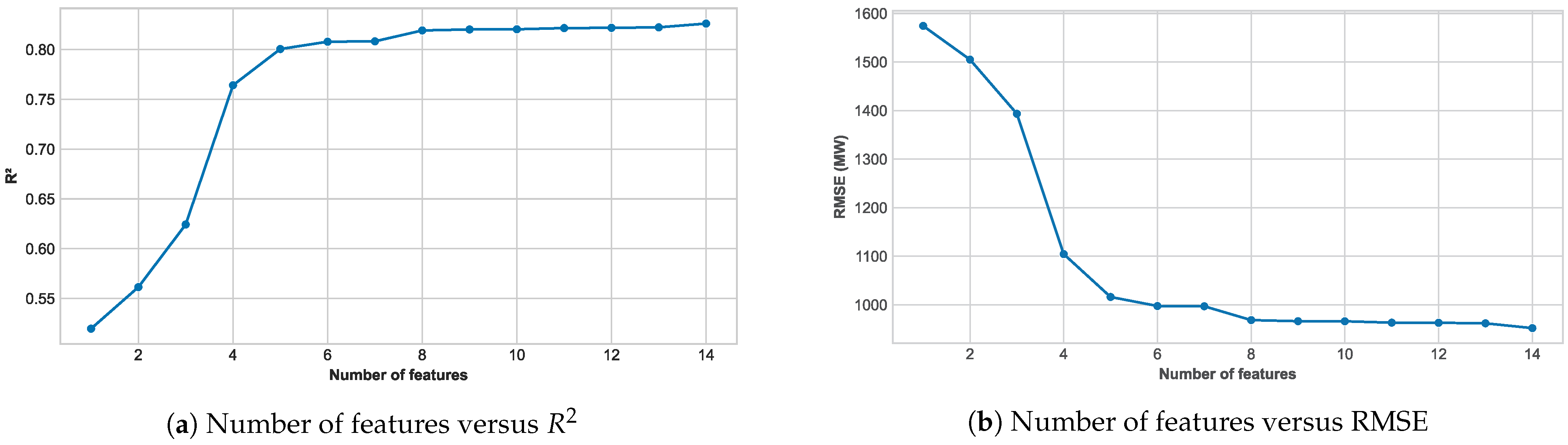
Five key features are selected—last year’s cumulative PV capacity, population, agricultural land area, tertiary education, and electricity net consumption—which collectively account for 79% of the variation in PV capacity, to be fed into the models. Illustrated in Figure 1 is the relationship between the number of features, explained variation in PV capacity additions, and root mean squared error (RMSE) of the linear model used for feature selection. The analysis reveals marginal gains beyond these five features, with less than a 4% increase in explanatory power and no significant decrease in RMSE. Table A3 shows summary statistics for the selected features, and Table A4 shows the Pearson correlations between the selected features.
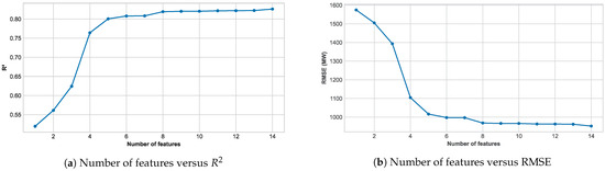
Figure 1.
Relationship between number of features and model performance metrics. (a) Number of features versus coefficient of determination, and (b) number of features versus root mean squared error after fitting a linear model. Features are numbered as follows: (1) tertiary education, (2) electricity net consumption, (3) agricultural land area, (4) previous year’s PV cumulative capacity, (5) population, (6) electricity net generation, (7) land area, (8) labour force, (9) fossil fuels electricity net generation, (10) rural land area, (11) primary education, (12) value added by agriculture, (13) forest area, (14) total unemployment.
A comparison of the results obtained from the developed models is presented in Table 2. Detailed equations describing these models can be found in Appendix B. The best results are achieved by the combined model, which has a global error value of 9.7%. The polynomial and neural network models perform similarly and have a global error of 18.8% and 18.4%, respectively. The OLS model has the highest global error of 36.1%, and despite having a higher test score compared to the polynomial and neural network models, its validation score is −1.57, which shows that its predictions are worse than a constant function that predicts the mean of PV capacity additions, deeming it unsuitable to model capacity additions. Considering that the error in measuring national PV capacity is at least [65], the combined model’s prediction error of 9.7% provides a reliable estimate of the actual capacity.
Table 2.
Comparison between the results of the different models. The training and test sets used in each model were identical.
Table A5 shows the importance of each feature in the combined model, the correlation between the features and the PV capacity additions, and how much variation each feature explains in the PV capacity additions. The interaction between the previous year’s PV cumulative capacity and the other features increased the correlation and explained more of the variation in the PV capacity additions compared to single features, which explains why these terms are the most important in the model. This also explains why the OLS model had the lowest training () compared to the other models, which had a much higher training (>0.96).
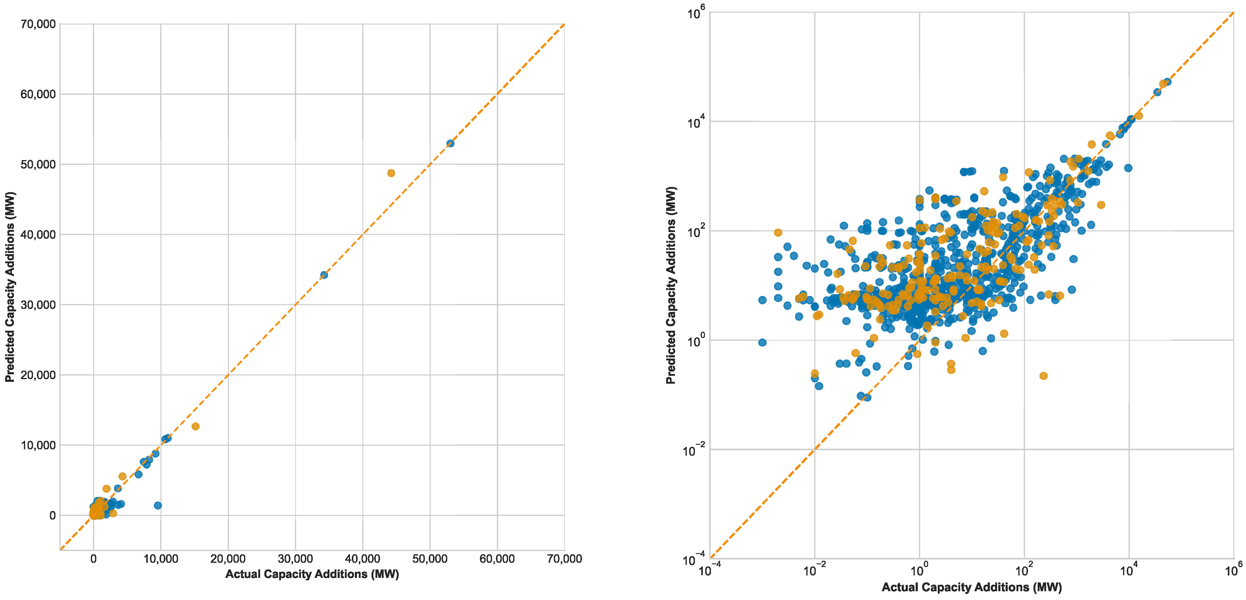
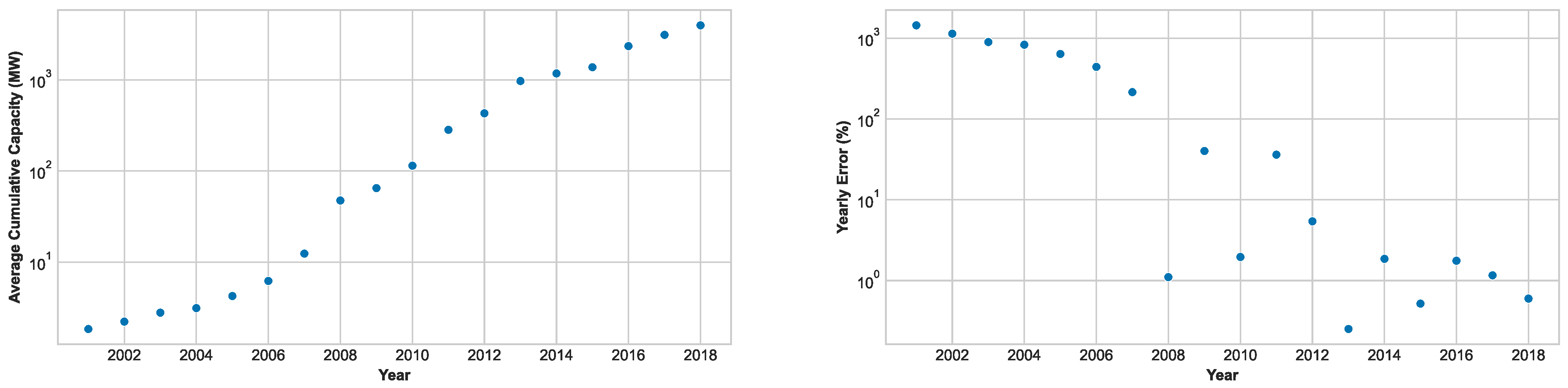
Figure 2 shows the linear and logarithmic actual versus predicted capacity additions for the combined model. The combined model is highly accurate for capacity additions greater than 1 GW (global error = 4.5%), has a medium accuracy for capacities between 1 MW and 1 GW (global error = 19.1%), and has a low accuracy for capacities below 1 MW (global error = 177%). Figure 3 shows the average cumulative PV capacity per year and the yearly error for the combined model. The error is highest in earlier years when the average capacity was low, but it drops significantly once the capacity starts to increase. This suggests that the model works well once a capacity threshold has been surpassed. This threshold is probably related to the state of the solar PV market.
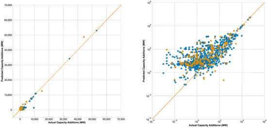
Figure 2.
Linear and logarithmic actual vs. predicted solar photovoltaic capacity additions for the combined model. Blue points represent the training set and orange points represent the test set.
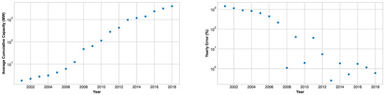
Figure 3.
Average cumulative solar photovoltaic capacity and error per year for the combined model. The yearly error was calculated from the entire dataset by dividing the mean absolute error per year by the average cumulative capacity that year.
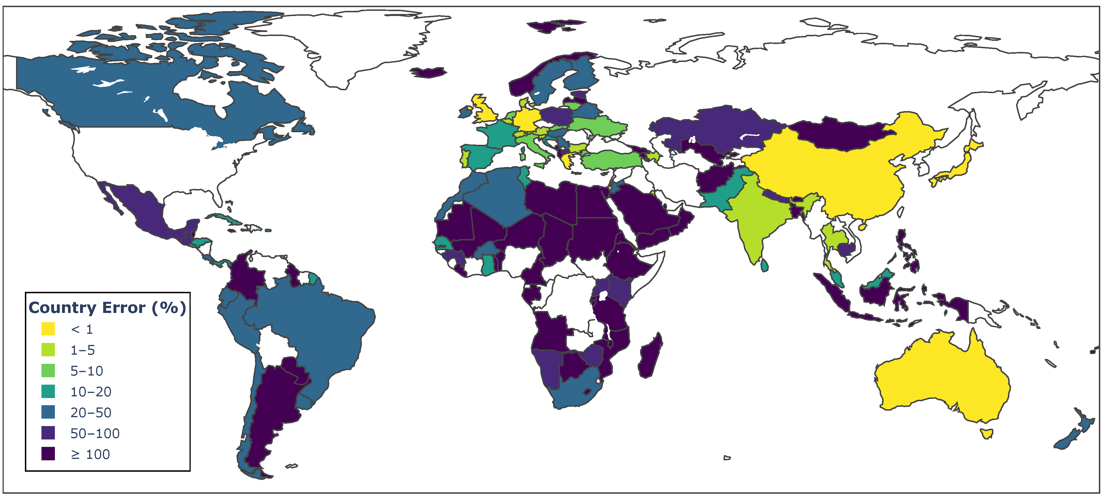
Figure 4 shows the country error for the combined model. The largest errors are for countries with low to no PV capacity additions, as shown in Figure 5. These countries increase the model’s global error to about 10%, but as shown in Figure 4, countries with high capacities have errors that are significantly smaller than 10%. For example, Germany, the United Kingdom, China, Australia, Greece, and Japan have an error of less than 1%. Portugal, India, Austria, Denmark, Bulgaria, Belgium, and Switzerland have an error of less than 5%. The model works well as a forecasting tool in countries with a mature solar PV market but performs less well in countries with emerging markets.
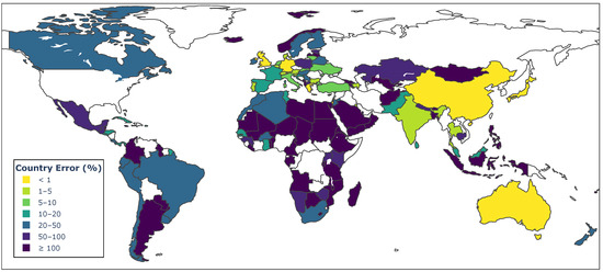
Figure 4.
Country error of the combined model, determined by dividing the mean absolute error per country by the respective mean cumulative photovoltaic capacity. Countries without available data are represented in white.

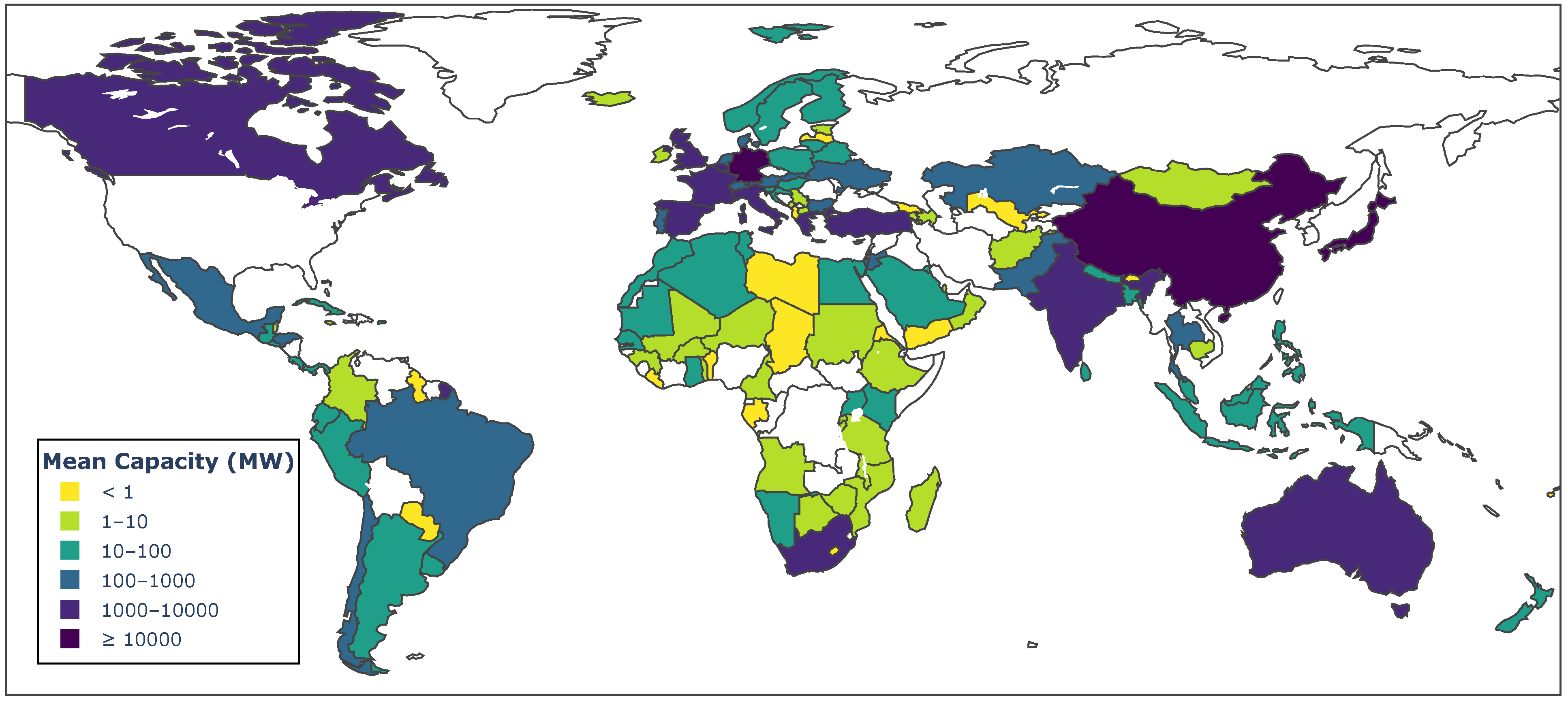
Figure 5.
Mean cumulative photovoltaic capacity across various countries from 2001 to 2018. Countries without available data are represented in white.
While the model may exhibit significant errors in certain countries, its appropriateness depends on the specific application at hand. For instance, when forecasting solar PV capacity for monitoring PV generation, an error of around 10% or less is typically acceptable. In the context of ranking countries’ PV deployment based on geographic factors, the observed error describes deviations from expected capacity additions compared to similar nations, offering valuable comparative insight. Lastly, when evaluating policy effectiveness using the model, discrepancies between actual and projected capacities can serve as indicators of policy impact, given the model’s inherent exclusion of policy inputs.
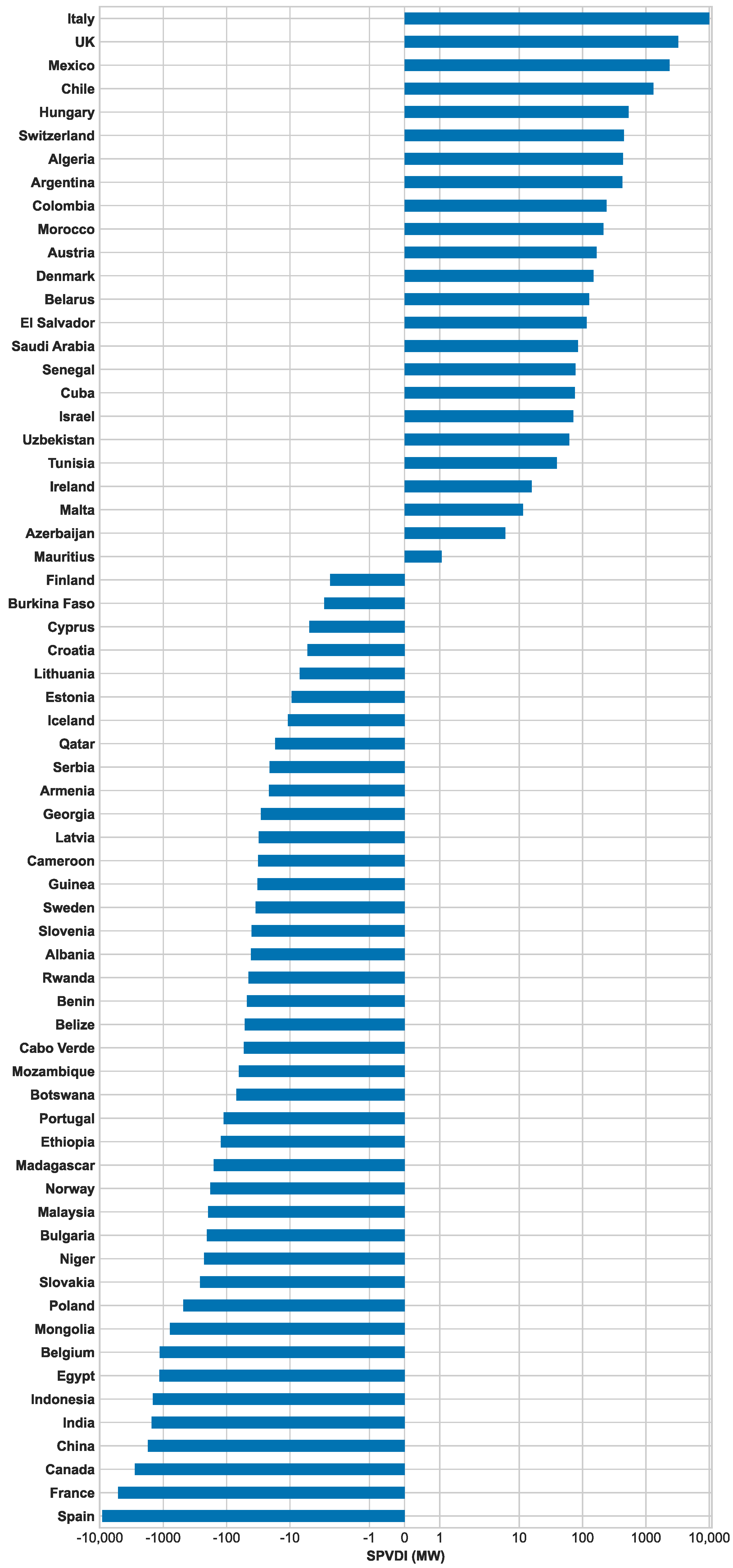
Figure 6 shows the solar PV deployment index (SPVDI) for countries during the period from 2010 to 2018. Notably, Italy installed more capacity than expected from similar countries by 10 GW, the United Kingdom by 3.2 GW, Mexico by 2.4 GW, Chile by 1.3 GW, and Hungary by 0.5 GW. On the other hand, Spain installed less than expected by 9.1 GW, France by 5.1 GW, Canada by 2.8 GW, China by 1.7 GW, and India by 1.5 GW.

Figure 6.
Solar PV deployment index (SPVDI) for different countries during the period from 2010 to 2018. Countries are ranked based on their solar photovoltaic deployment compared to other countries with similar social, economic, and land-use factors. A positive value indicates that a country has more capacity than expected, while a negative value means less capacity than expected from similar countries.
The top 10 countries in terms of PV deployment based on the SPVDI are Italy, the United Kingdom, Mexico, Chile, Hungary, Switzerland, Algeria, Argentina, Colombia, and Morocco. In contrast, the bottom 10 countries are Spain, France, Canada, China, India, Indonesia, Egypt, Belgium, Mongolia, and Poland. This does not necessarily imply that these countries are over- or underdeploying solar PV, as the index does not consider each country’s individual targets. Nonetheless, the SPVDI offers valuable insights into a country’s performance relative to others with similar geographic characteristics. Improving the index could involve integrating each nation’s capacity targets; however, such data are often lacking for many countries and, when available, may not specifically pertain to solar PV but encompass renewable energy overall.
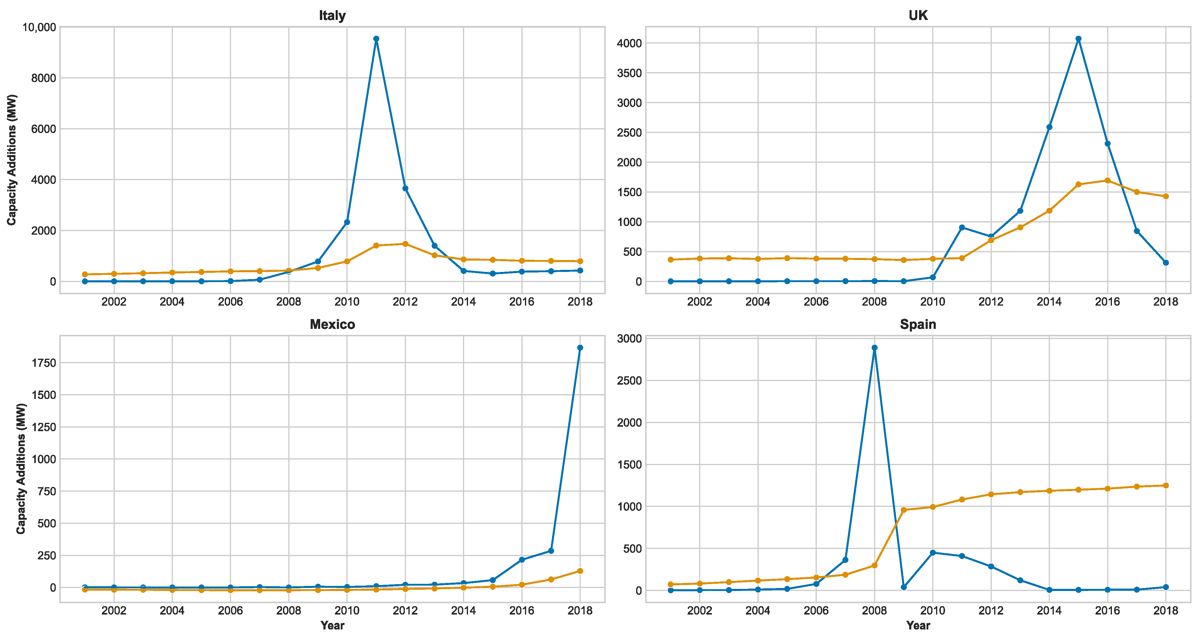
Figure 7 shows the actual versus estimated PV capacity additions for Italy, the United Kingdom, Mexico, and Spain from 2001 to 2018. Prior to 2008 in Italy, the actual capacity additions consistently fell short of expectations despite the implementation of the “Photovoltaic Roofs” program, which ran between 2001 and 2003 [66]. This initiative, offering up to 75% of installation costs for systems ranging from 1 kW to 20 kW connected to the distribution network [67], led to a deficit of 0.9 GW of installed capacity compared to what was expected. Feed-in tariff programs, “Conto Energia” (CE), were introduced in 2005, spanning five phases. The first CE, which ran between 2005 and 2006, achieved its 0.5 GW target [68]. Despite reaching the target, this phase led to a deficit of 0.7 GW compared to what was expected. The second CE was planned to last between 2007 and 2010, but it was extended to include PV systems installed before 31 December 2010 and operating before 30 June 2011, which led to a surge of investment to benefit from the feed-in tariffs [68]. The policy continued through the third CE, which entered into force in 2010 and was for PV systems commissioned between 1 January 2011 and 31 May 2011 [68]. The second and third CE programs were successful as they led to a surplus of 9.5 GW in installed capacity. The fourth CE program witnessed a significant reduction in tariffs on a monthly basis and expired in August 2012 [68]. The fourth CE was successful despite the significant reduction in rates as capacity additions were higher than expected by 10.3 GW. The fifth CE was introduced in 2012 and ended in 2013, during which capacity additions were higher than expected by 2.6 GW. Overall, the CE programs led to 11.3 GW of capacity additions above what was expected. Following the conclusion of the CE scheme, a new tax credit system was implemented in 2013 [68]. However, capacity additions in the subsequent years dropped below expectations by 1.8 GW.

Figure 7.
Actual versus estimated solar photovoltaic capacity additions for Italy, the United Kingdom, Mexico, and Spain for years between 2001 and 2018. Blue points represent actual capacity, while orange points represent estimated capacity.
In the United Kingdom, there are two main policies when it comes to solar PV: renewable obligation certificates (ROCs) for systems above 50 kW of rated power and feed-in tariffs (FIT) for systems below 5 MW of rated power [69,70]. ROCs were introduced in 2002 for England, Wales, and Scotland and in 2005 in Northern Ireland [71]. Despite the implementation of the scheme, capacity additions remained lower than expected until 2011, when the government declared that it would extend the scheme in England and Wales from 2027 to 2037 and would change it from a live-traded scheme to a fixed price certificate (FPC)-based scheme [71]. This increased capacity additions by 4.7 GW compared to the expected level until 2017 when the closure of the scheme [72] led to fewer additions than expected by 1.1 GW in the following year. The FIT scheme was launched in 2010 and ended in 2019. However, in 2016, a cap was applied to the number of new installations that could be accredited [69]. This led to fewer installations than expected by 1.8 GW in the next two years. Prior to this, the FIT scheme increased capacity additions by 5 GW compared to what was expected.
The actual additions are very close to the expected additions in Mexico up until the year 2015, after which capacity additions increased. This coincides with the introduction of long-term energy auctions. These auctions ran three times in 2015, 2016, and 2017. During these auctions, retailers would announce their requirement of capacity, consumption, or clean energy certificates, and generators would bid for them separately or in packages [73]. This led to more capacity than expected by 0.5 GW between 2015 and 2017. In 2018, major power consumers were required to buy 5% of electricity from power purchase agreements (PPAs) with clean power suppliers or through purchasing clean energy certificates [74], and the 15% customs duty on solar PV module imports which was introduced in 2015 was eliminated [75]. This led to more capacity additions by 1.7 GW compared to what was expected.
Spain introduced FITs in 1997. Generators could choose between fixed FITs that were adjusted annually or fixed premiums paid on top of the electricity market price. This was amended in 2004 so that FITs were set as a percentage of the electricity price and revised every 4 years [12], and were guaranteed to be paid for the lifetime of the solar power plants [76]. These policies had no significant impact on deployment, as capacity remained less than expected by 0.5 GW from 2001 to 2006. The FIT policy was revised again in 2007 so that FIT rates were fixed and updated every 4 years starting in 2010, or once 85% of the capacity target was reached, which ended up happening in the same year. This meant the government was going to lower the FIT rate, which led to a surge of investment to take advantage of the current FIT before the new tariff was implemented. During this period, capacity additions blew up and were higher than expected by 2.8 GW. The government responded by introducing policies that aimed to decrease deployment such as annual capacity quotas, the lifetime of FIT payments was reduced to 25 years for new plants, and FIT rates were reduced for small- and medium-sized solar PV. Further policies were introduced in 2010 such as limiting running hours eligible for FIT payments, reducing the FIT lifetime to 25 years for all existing plants, and reducing FIT rates further. These measures were not enough, as the government had to implement additional measures in 2012 such as introducing a moratorium on support for new systems and revising FIT rates [12]. Finally, a sun tax was introduced in 2014 which aimed to cover the cost of balancing the grid [77]. All of these measures reduced additions to less than expected by 10.1 GW in the period between 2009 and 2018.
5. Conclusions
The previous year’s cumulative PV capacity, population, agricultural land area, tertiary education, and electricity net consumption are identified as key features in explaining solar PV deployment. Using these features, the model achieves a global error of less than 10%. With country errors also below 10% in many cases, the model serves as a reliable forecasting tool across various nations.
Furthermore, the solar PV deployment index provides governments and policy makers with a benchmark for evaluating a country’s performance relative to others with similar social, economic, and land-use characteristics. This index could aid in setting feasible solar PV targets. Additionally, the model offers a means to assess the efficacy of solar PV policies by comparing actual deployment against expected figures. Such analysis can inform policy refinement and enhance the likelihood of achieving national targets.
Future research should concentrate on enhancing model accuracy for countries with low capacity additions, extending its forecasting utility to these regions. Lastly, investigating the correlation between geographic factors and solar PV capacity types (residential, commercial, utility scale) presents an intriguing avenue for future exploration.
Author Contributions
Conceptualisation, H.A. and A.B.; methodology, H.A. and A.B.; formal analysis, H.A.; data curation, H.A.; writing—original draft preparation, H.A.; writing—review and editing, A.B.; visualization, H.A.; supervision, A.B. All authors have read and agreed to the published version of the manuscript.
Funding
This research received no external funding.
Data Availability Statement
The dataset used for the analysis is publicly available and has been compiled from various open-source data sources. The compiled dataset, along with the code used for analysis, is accessible at: https://github.com/hussahalghanem/Forecasting-Global-PV-Installed-Capacity.git.
Acknowledgments
Hussah Alghanem would like to thank Imam Abdulrahman Bin Faisal University and the Government of Saudi Arabia for her PhD scholarship.
Conflicts of Interest
The authors declare no conflicts of interest.
Abbreviations
The following abbreviations are used in this manuscript:
| PV | photovoltaic |
| GW | gigawatt |
| WEM | World Energy Model |
| MAPE | mean absolute percentage error |
| GDP | gross domestic product |
| GNI | gross national income |
| MWh | megawatt hour |
| REC | renewable energy certificate |
| IEA | International Energy Agency |
| CMCC | Euro-Mediterranean Center on Climate Change |
| IRENA | International Renewable Energy Agency |
| EIA | Energy Information Administration |
| REN21 | Renewable Energy Policy Network For The 21st Century |
| coefficient of determination | |
| PCA | principal component analysis |
| RMSE | root mean square error |
| MLP | multilayer perceptron |
| MAE | Mean absolute error |
| MSE | mean squared error |
| MW | megawatt |
| kWh | kilowatt hour |
| OLS | ordinary least squares |
| W | watt |
| KOFGI | KOF Globalisation Index |
| GHI | global horizontal irradiance |
Appendix A
Table A1.
Number of data points used in the analysis presented in Table 1 to examine the correlation between each factor and solar PV capacity additions.
Table A1.
Number of data points used in the analysis presented in Table 1 to examine the correlation between each factor and solar PV capacity additions.
| Feature | N |
|---|---|
| Last year’s PV cumulative capacity (MW) | 4320 |
| Solar PV module cost (2019 USD per W) | 4320 |
| Land area (km2) | 3948 |
| Cloud coverage (%) | 3948 |
| Daylight hours (min/day) | 3948 |
| Precipitation (mm/h) | 3948 |
| Snowfall (mm/h) | 3948 |
| Temperature (°C) | 3948 |
| Population | 3939 |
| Forest area (km2) | 3939 |
| Average theoretical potential GHI (kWh/m2/day) | 3864 |
| GDP (current USD) | 3857 |
| GNI (current USD) | 3765 |
| KOFGI | 3718 |
| Agriculture, forestry, and fishing, value added (current USD) | 3686 |
| Labour force | 3675 |
| Total unemployment | 3675 |
| Access to electricity (% of population) | 3655 |
| Industry (including construction), value added (current USD) | 3646 |
| Manufacturing, value added (current USD) | 3556 |
| Agricultural land (km2) | 3549 |
| Nuclear electricity net generation (billion kWh) | 3538 |
| Duration of compulsory education (years) | 3444 |
| Electricity net generation (billion kWh) | 3433 |
| Fossil fuels electricity net generation (billion kWh) | 3412 |
| Electricity net consumption (billion kWh) | 3400 |
| Urban land area (km2) | 3381 |
| Rural land area (km2) | 3381 |
| Primary education | 3028 |
| Secondary education | 2601 |
| Tertiary education | 2367 |
| Research and development expenditure (% of GDP) | 1603 |
| Gini index (World Bank estimate) | 1295 |
| Public investments in solar energy (2019 million USD) | 1001 |
| Investment in energy with private participation (current USD) | 754 |
| Ease of doing business rank | 178 |
Table A2.
Summary the characteristics of principal component analysis (PCA) clusters, including the number of variables within each cluster, the coefficient of determination (R2) obtained when fitting cluster variables into a linear model with PV capacity additions, and the corresponding number of data points used in the fitting process.
| Cluster | Number of Features within Each Cluster | N | |
|---|---|---|---|
| 1 | 10 | 0.769 | 2257 |
| 2 | 6 | 0.211 | 21 |
| 3 | 5 | 0.222 | 570 |
| 4 | 7 | 0.463 | 1763 |
| 5 | 2 | 0.002 | 3760 |
| 6 | 4 | 0.163 | 327 |
| 7 | 2 | 0.010 | 3125 |
Table A3.
Descriptive statistics of the features used in the models. This table shows the count, mean, standard deviation, and distribution quartiles of the selected features.
Table A3.
Descriptive statistics of the features used in the models. This table shows the count, mean, standard deviation, and distribution quartiles of the selected features.
| Added PV Capacity (MW) | Last Year’s PV Cumulative Capacity (MW) | Population | Agricultural Land (km2) | Tertiary Education | Electricity Net Consumption (Billion kWh) | |
|---|---|---|---|---|---|---|
| count | ||||||
| mean | ||||||
| std | ||||||
| min | 0 | |||||
| 25% | 0 | 0 | ||||
| 50% | ||||||
| 75% | ||||||
| max |
Table A4.
Pearson correlation coefficients among selected variables used as inputs for the models.
Table A4.
Pearson correlation coefficients among selected variables used as inputs for the models.
| Added Capacity (MW) | Last Year’s Cumulative Capacity (MW) | Population | Agricultural Land (km2) | Tertiary Education | Electricity Net Consumption (Billion kWh) | |
|---|---|---|---|---|---|---|
| Added capacity (MW) | 1.00 | 0.79 | 0.42 | 0.39 | 0.70 | 0.72 |
| Last year’s cumulative capacity (MW) | 0.79 | 1.00 | 0.30 | 0.27 | 0.54 | 0.58 |
| Population | 0.42 | 0.30 | 1.00 | 0.74 | 0.88 | 0.77 |
| Agricultural land (km2) | 0.39 | 0.27 | 0.75 | 1.00 | 0.73 | 0.75 |
| Tertiary education | 0.70 | 0.54 | 0.88 | 0.73 | 1.00 | 0.92 |
| Electricity net consumption (billion kWh) | 0.72 | 0.58 | 0.77 | 0.75 | 0.92 | 1.00 |
Table A5.
Feature importance, correlation, and variation explained by the combined model features. The main effect measures the contribution of the feature alone, while the total effect measures the contribution of the feature alone and in combination with other features.
Table A5.
Feature importance, correlation, and variation explained by the combined model features. The main effect measures the contribution of the feature alone, while the total effect measures the contribution of the feature alone and in combination with other features.
| Feature | Main Effect | Total Effect | Correlation with Capacity Additions | |
|---|---|---|---|---|
| Last year’s PV cumulative capacity (MW) * agricultural land (km2) | 0.13 | 0.72 | 0.95 | 0.90 |
| Last year’s PV cumulative capacity (MW)2 | 0.04 | 0.42 | 0.81 | 0.65 |
| Last year’s PV cumulative capacity (MW) * population | 0.06 | 0.26 | 0.97 | 0.93 |
| Last year’s PV cumulative capacity (MW) * electricity net consumption (billion kWh) | 0.05 | 0.23 | 0.96 | 0.92 |
| Agricultural land (km2) * electricity net consumption (billion kWh) | 0.10 | 0.21 | 0.65 | 0.42 |
| Last year’s PV cumulative capacity (MW) * tertiary education | 0.04 | 0.20 | 0.96 | 0.93 |
| Electricity net consumption (billion kWh)2 | 0.03 | 0.18 | 0.77 | 0.60 |
| Population * electricity net consumption (billion kWh) | 0.05 | 0.18 | 0.67 | 0.45 |
| Agricultural land (km2)2 | 0.09 | 0.09 | 0.36 | 0.19 |
| Population * agricultural land (km2) | 0.06 | 0.08 | 0.46 | 0.22 |
| Agricultural land (km2) * tertiary education | 0.04 | 0.06 | 0.71 | 0.51 |
| Electricity net consumption (billion kWh) | 0.05 | 0.05 | 0.67 | 0.45 |
| Population2 | 0.05 | 0.05 | 0.43 | 0.18 |
| Population | 0.05 | 0.05 | 0.40 | 0.16 |
| Agricultural land (km2) | 0.04 | 0.04 | 0.36 | 0.13 |
| Tertiary education2 | 0.04 | 0.04 | 0.85 | 0.71 |
| Tertiary education * electricity net consumption (billion kWh) | 0.02 | 0.02 | 0.83 | 0.69 |
| Population * tertiary education | 0.02 | 0.02 | 0.69 | 0.47 |
| Tertiary education | 0.02 | 0.02 | 0.67 | 0.45 |
| Last year’s PV cumulative capacity (MW) | 0.02 | 0.02 | 0.70 | 0.48 |
Appendix B
Appendix B.1. OLS Model
The following equation is used to estimate solar PV capacity additions for the OLS model:
where PV is the previous year’s cumulative PV capacity, POP is population, AL is agricultural land area, ED is tertiary education, and EC is electricity net consumption.
Appendix B.2. Polynomial Model
The following equation is used to estimate solar PV capacity additions for the polynomial model:
where PV is the previous year’s cumulative PV capacity, POP is population, AL is agricultural land area, ED is tertiary education, and EC is electricity net consumption.
Appendix B.3. Neural Network Model
The following equation is used to estimate solar PV capacity additions for the neural network model:
where HH1, HH2, HH3, HH4, and HH5 are the nodes within the second hidden layer and are calculated as follows:
where H1, H2, H3, H4, and H5 are the nodes within the first hidden layer and are calculated as follows:
where PV is the previous year’s cumulative PV capacity, POP is population, AL is agricultural land area, ED is tertiary education, and EC is electricity net consumption.
Appendix B.4. Combined Model
The following equation is used to estimate solar PV capacity additions for the combined model:
where HH1, HH2, HH3, HH4, and HH5 are the nodes within the second hidden layer and are calculated as follows:
where H1, H2, H3, H4, and H5 are the nodes within the first hidden layer and are calculated as follows:
where PV is the previous year’s cumulative PV capacity, POP is population, AL is agricultural land area, ED is tertiary education, and EC is electricity net consumption.
References
- REN21. Renewables 2022 Global Status Report; Technical Report; REN21: Paris, France, 2022. [Google Scholar]
- IRENA. Renewable Power Generation Costs 2020; IRENA: Masdar City, United Arab Emirates, 2021. [Google Scholar]
- Ministry of Ecology and Environment (MEE). China’s Achievements, New Goals and New Measures for Nationally Determined Contributions (NDCs); Technical Report; Ministry of Ecology and Environment (MEE): Beijing, China, 2021.
- Agency for Natural Resources and Energy (ANRE). Outline of Strategic Energy Plan; Agency for Natural Resources and Energy (ANRE): Tokyo, Japan, 2021.
- Ministry of Economic Development (MISE) and Ministry of the Environment and Protection of Natural Resources and the Sea and Ministry of Infrastructure and Transport. Integrated National Energy and Climate Plan; Technical Report; European Commission: Brussels, Belgium, 2019. [Google Scholar]
- Federal Ministry For Economic Affairs and Climate Action (BMWK). Overview of the Easter Package; Federal Ministry For Economic Affairs and Climate Action (BMWK): Berlin/Bonn, Germany, 2022.
- Government of Spain. Draft of The Integrated National Energy and Climate Plan 2021–2030; Technical Report; European Commission: Brussels, Belgium, 2019. [Google Scholar]
- REN21. Renewables 2021 Global Status Report; Technical Report; REN21: Paris, France, 2021. [Google Scholar]
- Department of Public Enterprises (DPE). Roadmap for Eskom in a Reformed Electricity Supply Industry; Technical Report; Department of Public Enterprises (DPE): Arcadia, South Africa, 2019.
- REN21. Renewables 2020 Global Status Report; Technical Report; REN21: Paris, France, 2020. [Google Scholar]
- Brown, A.; Müller, S. Deploying Renewables 2011: Best and Future Policy Practice; Technical Report; International Energy Agency: Paris, France, 2011. [Google Scholar]
- del Río, P.; Mir-Artigues, P. A Cautionary Tale: Spain’s Solar PV Investment Bubble; Technical Report; International Institute for Sustainable Development: Winnipeg, Canada, 2014. [Google Scholar]
- IISD. Mapping India’s Energy Policy 2022: Aligning Support and Revenues with a Net-Zero Future International Institute for Sustainable Development; Technical Report; International Institute for Sustainable Development: Winnipeg, Canada, 2022. [Google Scholar]
- Lolla, A.; Zieliński, M.; Analysis, M.E.; Edianto, A.S.; Jones, D. India’s Race to 175 GW; Technical Report; EMBER: London, UK, 2022. [Google Scholar]
- Department of Energy and Climate Change. Identifying Trends in the Deployment of Domestic Solar PV under the Feed-in Tariff Scheme; Technical Report; Department of Energy and Climate Change: London, UK, 2011.
- US Census Bureau. Glossary. Available online: https://www.census.gov/programs-surveys/geography/about/glossary.html#par_textimage_13 (accessed on 26 December 2022).
- Jan, I.; Ullah, W.; Ashfaq, M. Social acceptability of solar photovoltaic system in Pakistan: Key determinants and policy implications. J. Clean. Prod. 2020, 274, 123140. [Google Scholar] [CrossRef]
- Letchford, J.; Lakkaraju, K.; Vorobeychik, Y. Individual Household Modeling of Photovoltaic Adoption. In Proceedings of the AAAI 2014 Fall Symposium Series, Arlington, VA, USA, 13–15 November 2014. [Google Scholar]
- Aklin, M.; yo Cheng, C.; Urpelainen, J. Geography, community, household: Adoption of distributed solar power across India. Energy Sustain. Dev. 2018, 42, 54–63. [Google Scholar] [CrossRef]
- Graziano, M.; Gillingham, K. Spatial patterns of solar photovoltaic system adoption: The influence of neighbors and the built environmentz. J. Econ. Geogr. 2015, 15, 815–839. [Google Scholar] [CrossRef]
- Peralta, A.A.; Balta-Ozkan, N.; Longhurst, P. Spatio-temporal modelling of solar photovoltaic adoption: An integrated neural networks and agent-based modelling approach. Appl. Energy 2022, 305, 117949. [Google Scholar] [CrossRef]
- Yu, J.; Wang, Z.; Majumdar, A.; Rajagopal, R. DeepSolar: A Machine Learning Framework to Efficiently Construct a Solar Deployment Database in the United States. Joule 2018, 2, 2605–2617. [Google Scholar] [CrossRef]
- McEachern, M.; Hanson, S. Socio-geographic perception in the diffusion of innovation: Solar energy technology in Sri Lanka. Energy Policy 2008, 36, 2578–2590. [Google Scholar] [CrossRef]
- Mayer, K.; Wang, Z.; Arlt, M.L.; Neumann, D.; Rajagopal, R. DeepSolar for Germany: A deep learning framework for PV system mapping from aerial imagery. In Proceedings of the SEST 2020—3rd International Conference on Smart Energy Systems and Technologies, Istanbul, Turkey, 7–9 September 2020. [Google Scholar] [CrossRef]
- Liu, B.; Song, C.; Wang, Q.; Wang, Y. Forecasting of China’s solar PV industry installed capacity and analyzing of employment effect: Based on GRA-BiLSTM model. Environ. Sci. Pollut. Res. 2022, 29, 4557–4573. [Google Scholar] [CrossRef]
- IEA. World Energy Model Documentation; Technical Report; IEA: Paris, France, 2021. [Google Scholar]
- Haegel, N.M.; Margolis, R.; Buonassisi, T.; Feldman, D.; Froitzheim, A.; Garabedian, R.; Green, M.; Glunz, S.; Henning, H.M.; Holder, B.; et al. Terawatt-scale photovoltaics: Trajectories and challenges. Science 2017, 356, 141–143. [Google Scholar] [CrossRef]
- International Renewable Energy Agency. Global Energy Transformation: A Roadmap to 2050 (2019 Edition); International Renewable Energy Agency: Masdar City, United Arab Emirates, 2019. [Google Scholar]
- Ravishankar, R.; AlMahmoud, E.; Habib, A.; de Weck, O.L. Capacity Estimation of Solar Farms Using Deep Learning on High-Resolution Satellite Imagery. Remote Sens. 2023, 15, 210. [Google Scholar] [CrossRef]
- Hu, W.; Bradbury, K.; Malof, J.M.; Li, B.; Huang, B.; Streltsov, A.; Fujita, K.S.; Hoen, B. What you get is not always what you see—pitfalls in solar array assessment using overhead imagery. Appl. Energy 2022, 327, 120143. [Google Scholar] [CrossRef]
- Ren, S.; Malof, J.; Fetter, R.; Beach, R.; Rineer, J.; Bradbury, K. Utilizing Geospatial Data for Assessing Energy Security: Mapping Small Solar Home Systems Using Unmanned Aerial Vehicles and Deep Learning. ISPRS Int. J. Geo-Inf. 2022, 11, 222. [Google Scholar] [CrossRef]
- Imran, A.; Zhu, Q.; Sulaman, M.; Bukhtiar, A.; Xu, M. Electric-Dipole Gated Two Terminal Phototransistor for Charge-Coupled Device. Adv. Opt. Mater. 2023, 11, 2300910. [Google Scholar] [CrossRef]
- Suri, M.; Betak, J.; Rosina, K.; Chrkavy, D.; Suriova, N.; Cebecauer, T.; Caltik, M.; Erdelyi, B. Global Photovoltaic Power Potential by Country; Technical Report; World Bank: Washington, DC, USA, 2020. [Google Scholar]
- IEA; CMCC. Weather for Energy Tracker. Available online: https://www.iea.org/articles/weather-for-energy-tracker (accessed on 7 August 2022).
- World Bank. World Bank Open Data; World Bank: Washington, DC, USA, 2022. [Google Scholar]
- IRENA. Data & Statistics. Available online: https://www.irena.org/Statistics (accessed on 16 January 2022).
- EIA. International Electricity Data. Available online: https://www.eia.gov/international/data/world (accessed on 6 April 2022).
- UNESCO Institute for Statistics. Data for the Sustainable Development Goals. Available online: http://uis.unesco.org/ (accessed on 22 March 2022).
- World Bank. Labor Force. Available online: https://data.worldbank.org/indicator/SL.TLF.TOTL.IN (accessed on 22 March 2022).
- International Labour Organization (ILOSTAT). ILOSTAT Database. Available online: https://ilostat.ilo.org/data/ (accessed on 11 April 2022).
- World Bank. Population, Total. Available online: https://data.worldbank.org/indicator/SP.POP.TOTL (accessed on 21 March 2022).
- Gygli, S.; Haelg, F.; Potrafke, N.; Sturm, J.E. The KOF Globalisation Index—Revisited. Rev. Int. Organ. 2019, 14, 543–574. [Google Scholar] [CrossRef]
- Dreher, A. Does globalization affect growth? Evidence from a new index of globalization. Appl. Econ. 2006, 38, 1091–1110. [Google Scholar] [CrossRef]
- World Bank. Agriculture, Forestry, and Fishing, Value Added (Current USD)| Data. Available online: https://data.worldbank.org/indicator/NV.AGR.TOTL.CD (accessed on 30 March 2022).
- OECD. OECD National Accounts Data; OECD: Paris, France, 2022. [Google Scholar]
- World Bank. Manufacturing, Value Added (Current USD). Available online: https://data.worldbank.org/indicator/NV.IND.MANF.CD (accessed on 30 March 2022).
- World Bank. Industry (Including Construction), Value Added (Current USD). Available online: https://data.worldbank.org/indicator/NV.IND.TOTL.CD (accessed on 30 March 2022).
- World Bank. GDP (Current USD). Available online: https://data.worldbank.org/indicator/NY.GDP.MKTP.CD?view=chart (accessed on 22 March 2022).
- OECD. Gross Domestic Product (GDP) (Indicator); OECD: Paris, France, 2022. [Google Scholar] [CrossRef]
- World Bank. GNI (Current USD). Available online: https://data.worldbank.org/indicator/NY.GNP.MKTP.CD?view=chart (accessed on 22 March 2022).
- OECD. Gross National Income (Indicator); OECD: Paris, France, 2022. [Google Scholar] [CrossRef]
- World Bank. Ease of Doing Business Rank. Available online: https://data.worldbank.org/indicator/IC.BUS.EASE.XQ (accessed on 23 March 2022).
- IRENA. Public Investment Trends in Renewables Dataset. Available online: https://www.irena.org/Statistics/View-Data-by-Topic/Finance-and-Investment/Renewable-Energy-Finance-Flows (accessed on 11 February 2022).
- Lafond, F.; Bailey, A.G.; Bakker, J.D.; Rebois, D.; Zadourian, R.; Mcsharry, P.; Farmer, J.D. How well do experience curves predict technological progress? A method for making distributional forecasts. Technol. Forecast. Soc. Chang. 2017, 128, 104–117. [Google Scholar] [CrossRef]
- World Bank; International Energy Agency (IEA); International Renewable Energy Agency (IRENA); United Nations Statistics Division (UNSD); World Health Organization (WHO). World Bank Global Electrification Database. Available online: https://trackingsdg7.esmap.org/ (accessed on 22 March 2022).
- World Bank. Private Participation in Infrastructure Project Database. Available online: http://ppi.worldbank.org (accessed on 11 March 2022).
- World Bank. Gini Index. Available online: https://data.worldbank.org/indicator/SI.POV.GINI?view=chart (accessed on 23 March 2022).
- Center for International Earth Science and Information Network—CIESIN—Columbia University. Low Elevation Coastal Zone (LECZ) Urban-Rural Population and Land Area Estimates, Version 2; NASA Socioeconomic Data and Applications Center (SEDAC): Palisades, NY, USA, 2013. [Google Scholar] [CrossRef]
- World Bank. Agricultural Land (sq. km). Available online: https://data.worldbank.org/indicator/AG.LND.AGRI.K2 (accessed on 22 March 2022).
- World Bank. Land Area (sq. km). Available online: https://data.worldbank.org/indicator/AG.LND.TOTL.K2?view=chart (accessed on 21 March 2022).
- World Bank. Forest Area (sq. km). Available online: https://data.worldbank.org/indicator/AG.LND.FRST.K2?view=chart (accessed on 22 March 2022).
- Pedregosa, F.; Varoquaux, G.; Gramfort, A.; Michel, V.; Thirion, B.; Grisel, O.; Blondel, M.; Prettenhofer, P.; Weiss, R.; Dubourg, V.; et al. Scikit-learn: Machine Learning in Python. J. Mach. Learn. Res. 2011, 12, 2825–2830. [Google Scholar]
- Gotwalt, C.M. JMP Neural Network Methodology; Technical Report; SAS Institute: Cary, NC, USA, 2023. [Google Scholar]
- Hastie, T.; Tibshirani, R.; Friedman, J. The Elements of Statistical Learning; Springer: New York, NY, USA, 2001. [Google Scholar]
- Huxley, O.; Taylor, J.; Everard, A.; Briggs, J.; Tilley, K.; Harwood, J.; Buckley, A. The uncertainties involved in measuring national solar photovoltaic electricity generation. Renew. Sustain. Energy Rev. 2022, 156, 112000. [Google Scholar] [CrossRef]
- Photovoltaic Roofs Programme—ETA-Florence. Available online: https://new.etaflorence.it/projects/photovoltaic-roofs-programme/ (accessed on 2 January 2024).
- Italian Government. Photovoltaic Roofs Program. Available online: https://www.gazzettaufficiale.it/eli/id/2001/03/29/001A3359/sg (accessed on 11 December 2023).
- Orioli, A.; Gangi, A.D. Six-years-long effects of the Italian policies for photovoltaics on the grid parity of grid-connected photovoltaic systems installed in urban contexts. Energy 2017, 130, 55–75. [Google Scholar] [CrossRef]
- Ofgem. Feed-in Tariffs (FIT). Available online: https://www.ofgem.gov.uk/environmental-and-social-schemes/feed-tariffs-fit (accessed on 7 January 2024).
- Dusonchet, L.; Telaretti, E. Comparative economic analysis of support policies for solar PV in the most representative EU countries. Renew. Sustain. Energy Rev. 2015, 42, 986–998. [Google Scholar] [CrossRef]
- Department for Energy Security and Net Zero. Renewables Obligation Call for Evidence on Introducing Fixed Price Certificates into the UK-Wide Renewables Obligation Schemes; Technical Report; Department for Energy Security and Net Zero: London, UK, 2023.
- Ofgem. Renewables Obligation (RO)—RO Closure|Ofgem. Available online: https://www.ofgem.gov.uk/environmental-and-social-schemes/renewables-obligation-ro/ro-closure (accessed on 21 December 2022).
- AURES II. Auctions for the Support of Renewable Energy in Mexico. 2019. Available online: http://aures2project.eu/wp-content/uploads/2019/12/AURES_II_case_study_Mexico.pdf (accessed on 8 January 2024).
- del Río, P. Auctions for Renewable Support in Mexico: Instruments and Lessons Learnt. 2017. Available online: http://aures2project.eu/wp-content/uploads/2021/07/mexico_final.pdf (accessed on 8 January 2024).
- Bellini, E. Mexico Eliminates 15% Customs Duties on Solar Module Imports—PV Magazine International. Available online: https://www.pv-magazine.com/2018/06/18/mexico-eliminates-15-customs-duties-on-solar-module-imports/ (accessed on 8 January 2024).
- Duffield, J.S.; Daskalopoulou, I.; Stricker, L.; Baruffini, M.; Kilci, E.N.; Pawełek, B. The politics of renewable power in Spain. Eur. J. Gov. Econ. 2020, 9, 5–25. [Google Scholar] [CrossRef]
- Rosales-Asensio, E.; de Simón-Martín, M.; Borge-Diez, D.; Pérez-Hoyos, A.; Santos, A.C. An expert judgement approach to determine measures to remove institutional barriers and economic non-market failures that restrict photovoltaic self-consumption deployment in Spain. Sol. Energy 2019, 180, 307–323. [Google Scholar] [CrossRef]
Disclaimer/Publisher’s Note: The statements, opinions and data contained in all publications are solely those of the individual author(s) and contributor(s) and not of MDPI and/or the editor(s). MDPI and/or the editor(s) disclaim responsibility for any injury to people or property resulting from any ideas, methods, instructions or products referred to in the content. |
© 2024 by the authors. Licensee MDPI, Basel, Switzerland. This article is an open access article distributed under the terms and conditions of the Creative Commons Attribution (CC BY) license (https://creativecommons.org/licenses/by/4.0/).