
Short-Term Electric Load Forecasting Based on Signal Decomposition and Improved TCN Algorithm
Abstract
:1. Introduction
2. Methodology
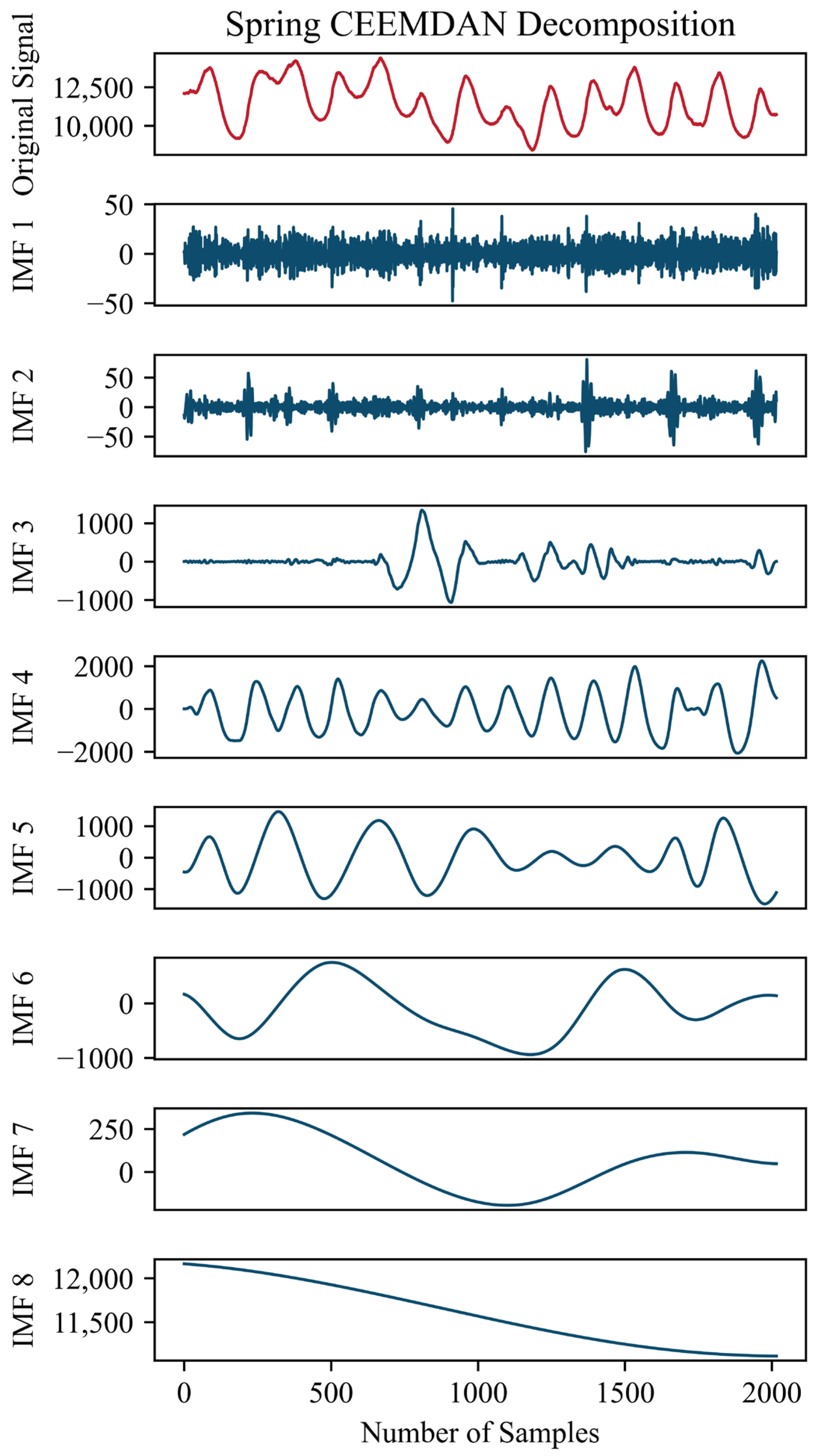
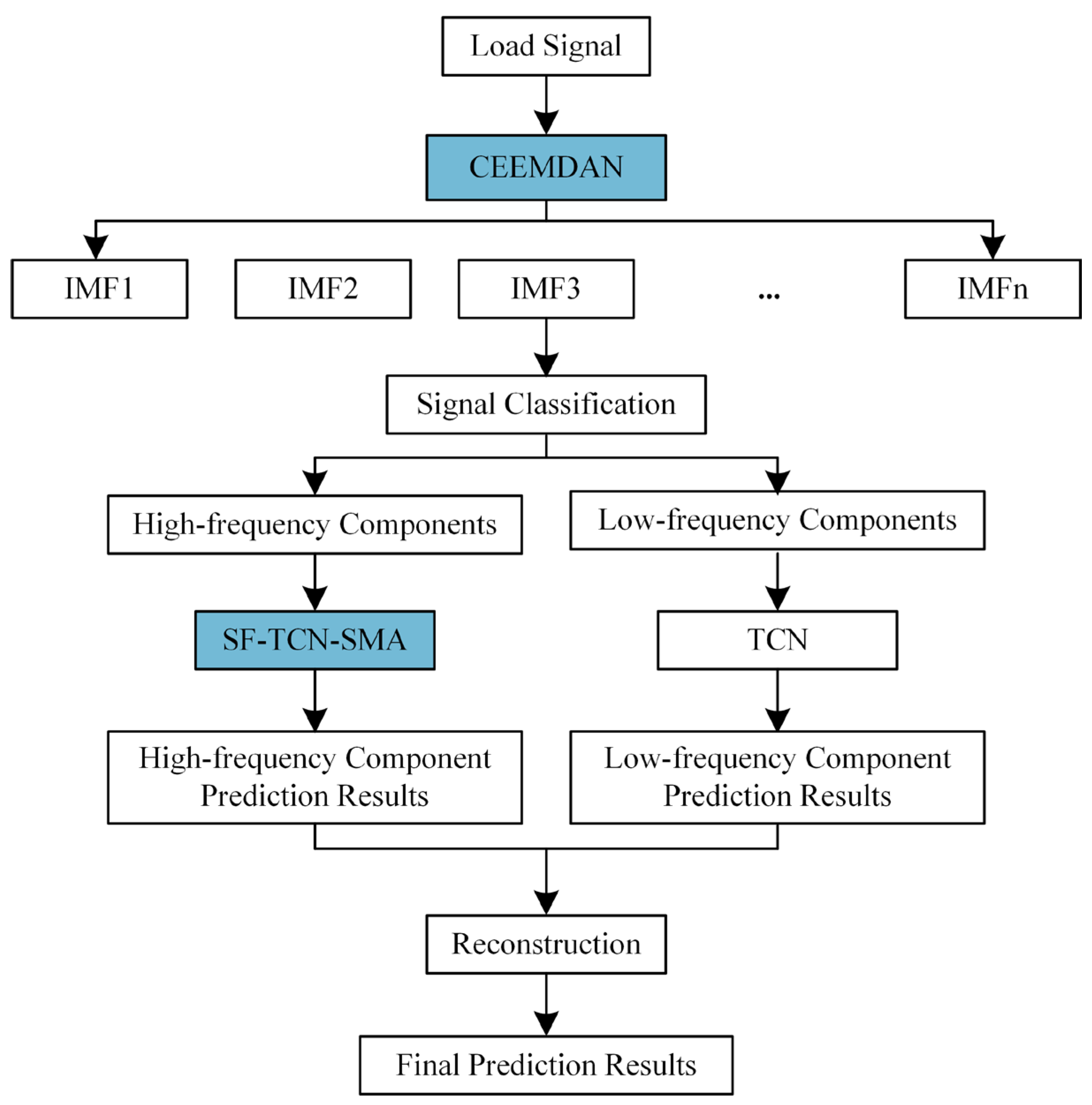
2.1. CEEMDAN
- Add white noise to the original signal to obtain :where is the amplitude coefficient of white noise, and is standard white noise.
- Use EMD to decompose the first set of and obtain the residual :where is the first-order intrinsic mode component, and is the number of trials.
- Use EMD on after adding adaptive noise to obtain the second-order modal component and the residual :where is the operator of the first-order intrinsic mode component.
- Repeat step (3), calculating the (k + 1)th order modal component and residual, until the residual becomes a monotonic function and can no longer be further decomposed into IMFs.
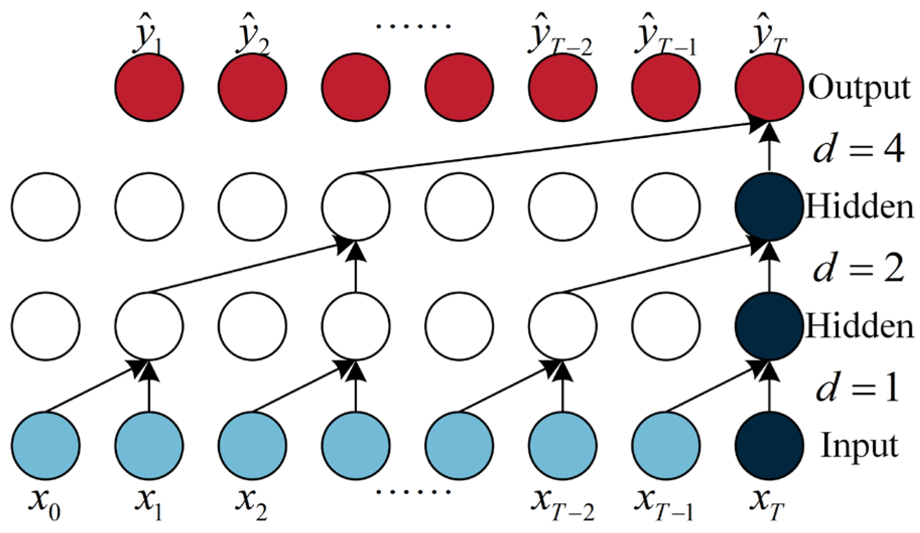
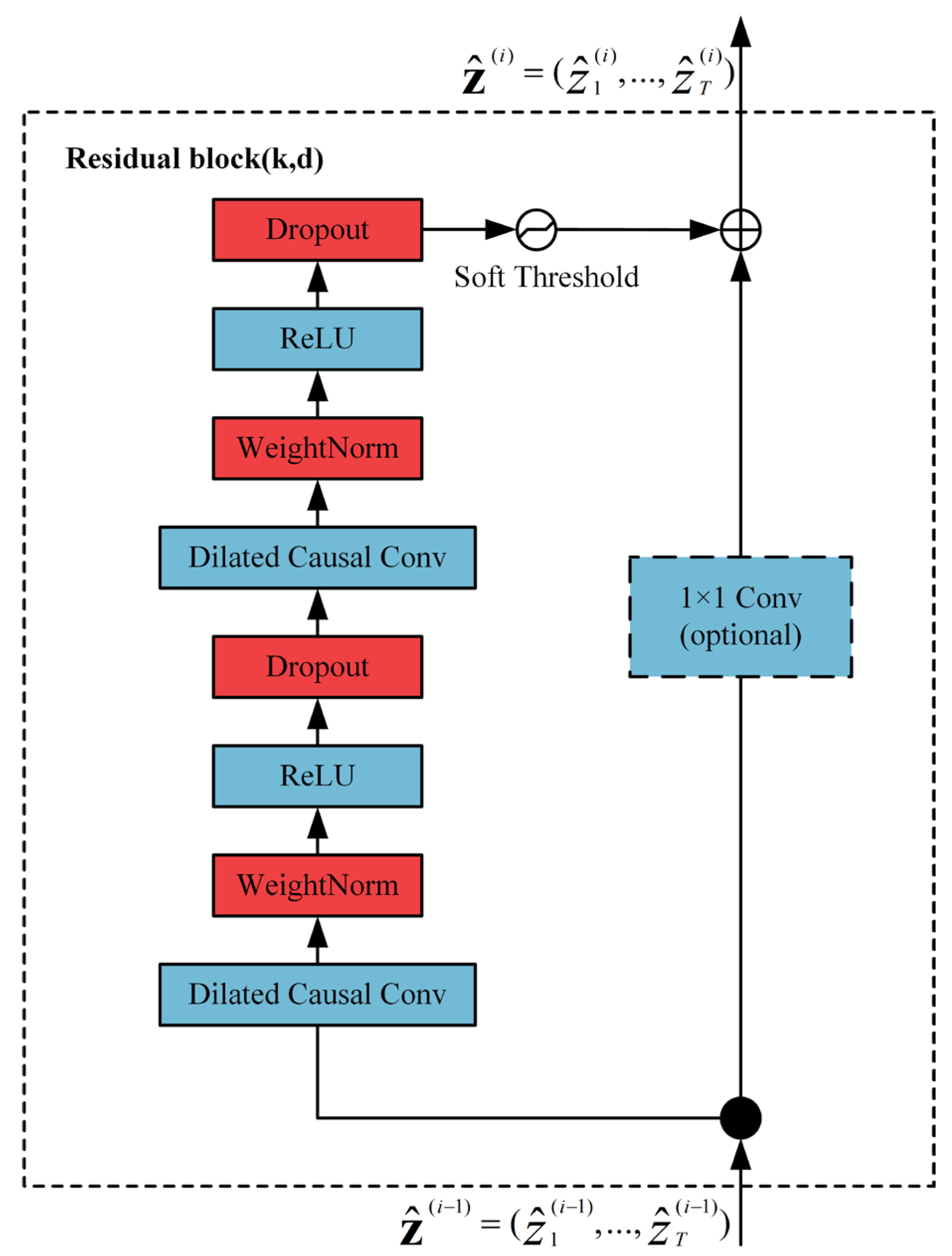
2.2. Principles of TCN and the Improved SF-TCN
2.3. Principles of SMA
- Approaching foodwhere , is a parameter that gradually decreases from 1 to 0; represents the current iteration number; indicates the position of the individual with the highest odor concentration, i.e., the position of the individual with the optimal fitness; represents the current position of the slime mold individual; and represent the positions of two randomly chosen slime mold individuals; and is a weight coefficient.The updated formula for is as follows:where represents the individual index in the slime mold population; represents the fitness of individual ; and indicates the best fitness obtained across all iterations.The formula of is , and its updated formula is as follows:The updated formula for is as follows:where , represents the best fitness achieved during the current iteration process; denotes the worst fitness achieved during the current iteration process; indicates that ranks in the top half of the group; and is a sequence of fitness values arranged in ascending order, used when addressing minimization problems.
- Encircling FoodDepending on the quality of the food, slime mold can adjust its search patterns. When the food concentration is high, it places more emphasis on that area; conversely, when the food concentration is low, it reduces the weight of that area and turns to explore other regions. The mathematical formula for updating the position of the slime mold is as follows:where and are the upper and lower bounds of the hyperparameter search, respectively; , acts as a control factor, which adjusts the balance between global search and local exploitation.
- Capturing FoodSlime mold employs biological oscillators to generate propagation waves that alter the flow of its cytoplasm, enabling it to search for and select food resources within its environment. By adjusting its oscillation frequency and engaging in random exploratory behavior, the slime mold adapts to varying concentrations of food, allowing the cells to more swiftly converge upon sources of high-quality food, while allocating a portion of its resources to the exploration of additional areas. The oscillation of parameters and their synergistic effect simulate the selective behavior of slime mold, empowering it to discover superior food sources and circumvent local optima. Despite facing numerous constraints during propagation, these very limitations afford the slime mold opportunities, enhancing its likelihood of locating high-quality food sources.
2.4. CEEMDAN-SF-TCN-SMA
3. Data Sources and Preprocessing
3.1. Data Sources
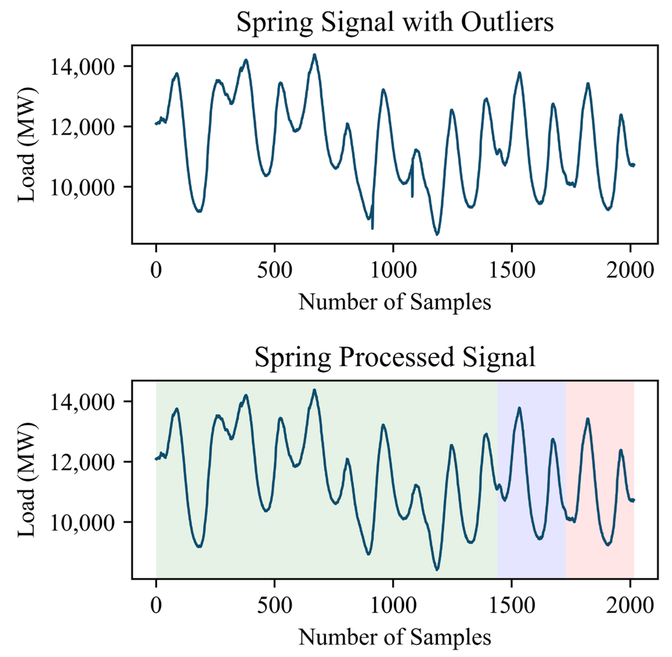
3.2. Data Preprocessing
4. Experiment and Results Analysis
4.1. Model Configuration and Evaluation Metrics
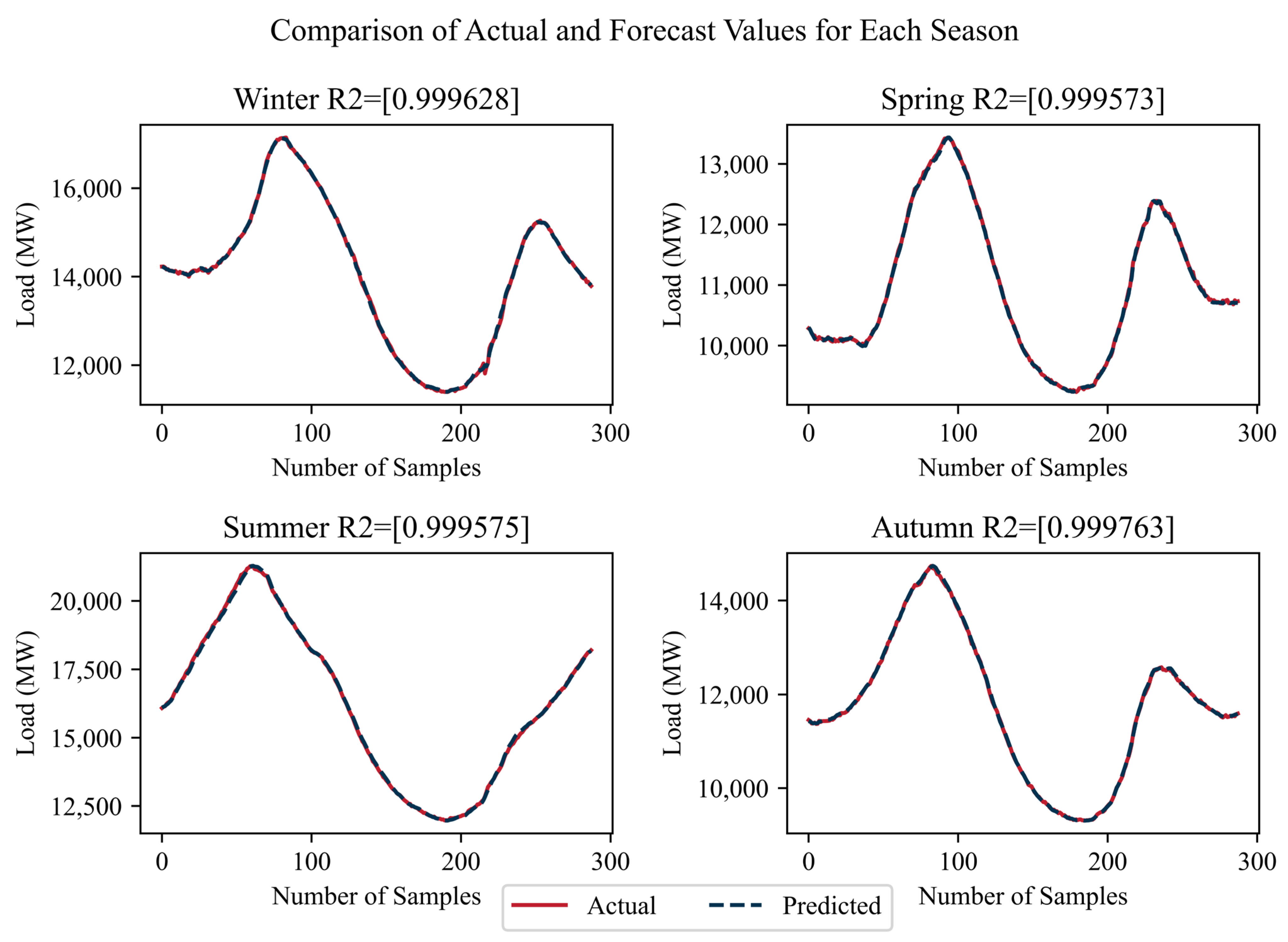
4.2. CEEMDAN-SF-TCN-SMA Forecasting Analysis
4.3. Comparative Analysis
5. Conclusions
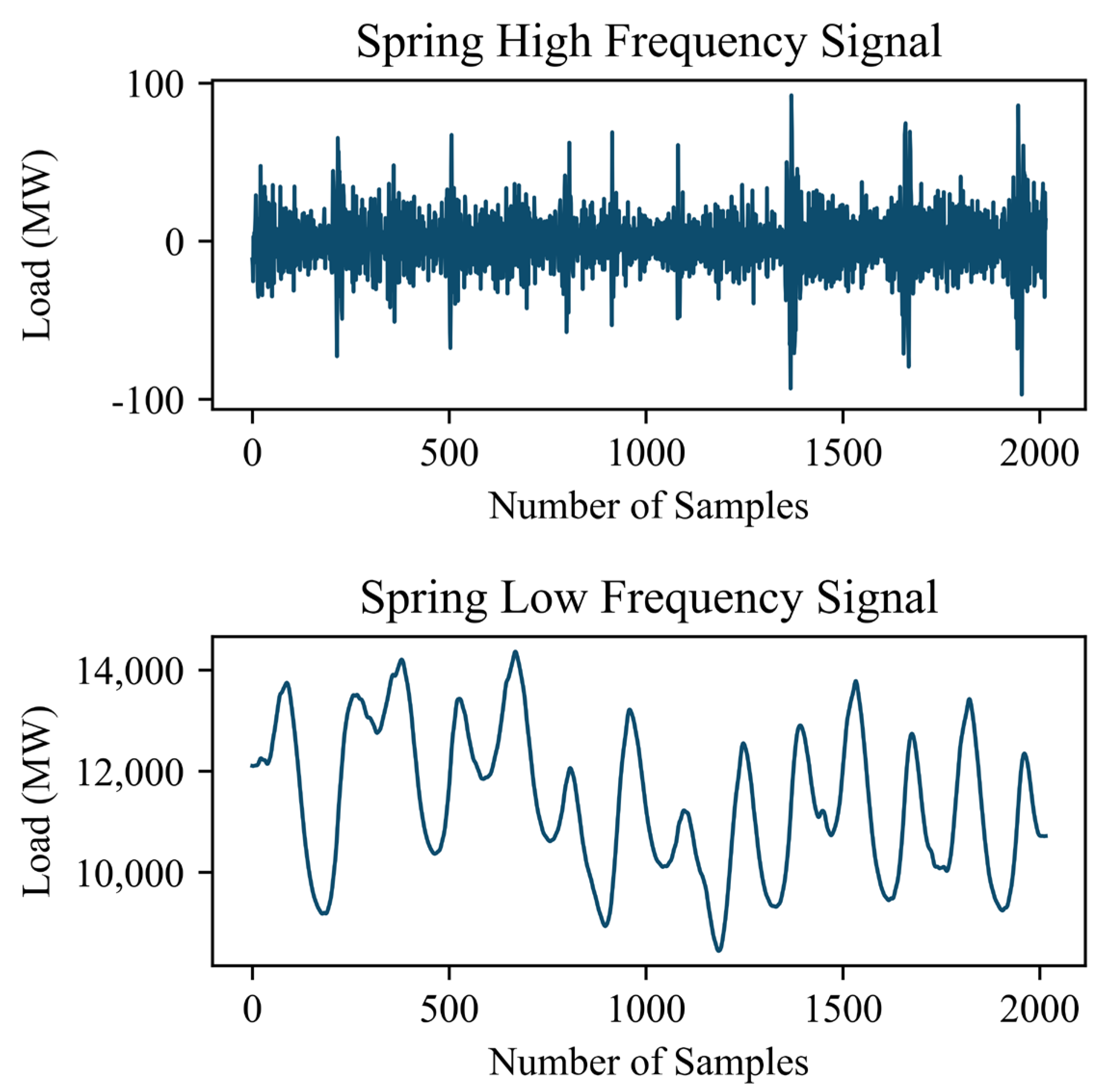
- By utilizing the CEEMDAN, our study effectively decomposes electric power load data into high-frequency and low-frequency components. This enables a more detailed analysis, capturing subtle fluctuations in the load curve that traditional methods may overlook.
- The introduction of an improved SF-TCN addresses the challenges in predicting high-frequency components. This model enhancement not only reduces the impact of noise but also improves the accuracy of short-term forecasts.
- The application of the shuffled memetic algorithm (SMA) for adjusting the neural network’s hyperparameters and soft thresholding enhances the neural network’s adaptability and forecasting ability.
- Our experimental results demonstrate that, compared to un-decomposed SVR, RNN, GRU, LSTM, CNN-LSTM, and TCN models as well as decomposed CEEMDAN-TCN and CEEMDAN-SF-TCN models, our method possesses superior forecasting capabilities.
Author Contributions
Funding
Data Availability Statement
Acknowledgments
Conflicts of Interest
References
- Chan, K.Y.; Yiu, K.F.C.; Kim, D.; Abu-Siada, A. Fuzzy Clustering-Based Deep Learning for Short-Term Load Forecasting in Power Grid Systems Using Time-Varying and Time-Invariant Features. Sensors 2024, 24, 1391. [Google Scholar] [CrossRef] [PubMed]
- Yin, C.; Wei, N.; Wu, J.; Ruan, C.; Luo, X.; Zeng, F. An Empirical Mode Decomposition-Based Hybrid Model for Sub-Hourly Load Forecasting. Energies 2024, 17, 307. [Google Scholar] [CrossRef]
- Kwon, B.S.; Park, R.J.; Song, K.B. Short-term load forecasting based on deep neural networks using LSTM layer. J. Electr. Eng. Technol. 2020, 15, 1501–1509. [Google Scholar] [CrossRef]
- Lee, C.M.; Ko, C.N. Short-term load forecasting using lifting scheme and ARIMA models. Expert Syst. Appl. 2011, 38, 5902–5911. [Google Scholar] [CrossRef]
- Taylor, J.W. Short-term load forecasting with exponentially weighted methods. IEEE Trans. Power Syst. 2011, 27, 458–464. [Google Scholar] [CrossRef]
- Xia, Y.; Yu, S.; Jiang, L.; Wang, L.; Lv, H.; Shen, Q. Application of fuzzy support vector regression machine in power load prediction. J. Intell. Fuzzy Syst. 2023, 45, 8027–8048. [Google Scholar] [CrossRef]
- Dong, X.; Deng, S.; Wang, D. A short-term power load forecasting method based on k-means and SVM. J. Ambient Intell. Humaniz. Comput. 2022, 13, 5253–5267. [Google Scholar] [CrossRef]
- Abumohsen, M.; Owda, A.Y.; Owda, M. Electrical load forecasting using LSTM, GRU, and RNN algorithms. Energies 2023, 16, 2283. [Google Scholar] [CrossRef]
- Zhang, J.; Huang, Y.; Pi, Y.; Sun, C.; Cai, W.; Huang, Y. Research on a Service Load Prediction Method Based on VMD-GLRT. Appl. Sci. 2023, 13, 3315. [Google Scholar] [CrossRef]
- Liu, M.; Qin, H.; Cao, R.; Deng, S. Short-Term Load Forecasting Based on Improved TCN and DenseNet. IEEE Access 2022, 10, 115945–115957. [Google Scholar] [CrossRef]
- Yao, H.; Tang, X.; Wei, H.; Zheng, G.; Yu, Y.; Li, Z. Modeling spatial-temporal dynamics for traffic prediction. arXiv 2018, arXiv:1803.01254. [Google Scholar]
- Guo, X.; Zhao, Q.; Zheng, D.; Ning, Y.; Gao, Y. A short-term load forecasting model of multi-scale CNN-LSTM hybrid neural network considering the real-time electricity price. Energy Rep. 2020, 6, 1046–1053. [Google Scholar] [CrossRef]
- Geng, G.; He, Y.; Zhang, J.; Qin, T.; Yang, B. Short-Term Power Load Forecasting Based on PSO-Optimized VMD-TCN-Attention Mechanism. Energies 2023, 16, 4616. [Google Scholar] [CrossRef]
- Smyl, S.; Dudek, G.; Pełka, P. Contextually enhanced ES-dRNN with dynamic attention for short-term load forecasting. Neural Netw. 2024, 169, 660–672. [Google Scholar] [CrossRef]
- Yang, Q.; Lin, Y.; Kuang, S.; Wang, D. A novel short-term load forecasting approach for data-poor areas based on K-MIFS-XGBoost and transfer-learning. Electr. Power Syst. Res. 2024, 229, 110151. [Google Scholar] [CrossRef]
- Nguyen, Q.D.; Nguyen, N.A.; Tran, N.T.; Solanki, V.K.; Crespo, R.G.; Nguyen, T.N.A. Online SARIMA applied for short-term electricity load forecasting. Preprint 2021. [Google Scholar] [CrossRef]
- Liu, M.; Li, Y.; Hu, J.; Wu, X.; Deng, S.; Li, H. A New Hybrid Model Based on SCINet and LSTM for Short-Term Power Load Forecasting. Energies 2024, 17, 95. [Google Scholar] [CrossRef]
- Tarmanini, C.; Sarma, N.; Gezegin, C.; Ozgonenel, O. Short term load forecasting based on ARIMA and ANN approaches. Energy Rep. 2023, 9, 550–557. [Google Scholar] [CrossRef]
- Xu, H.; Peng, Q.; Wang, Y.; Zhan, Z. Power-Load Forecasting Model Based on Informer and Its Application. Energies 2023, 16, 3086. [Google Scholar] [CrossRef]
- Torres, M.E.; Colominas, M.A.; Schlotthauer, G.; Flandrin, P. A complete ensemble empirical mode decomposition with adaptive noise. In Proceedings of the 2011 IEEE International Conference on Acoustics, Speech and Signal Processing (ICASSP), Prague, Czech Republic, 22–27 May 2011; IEEE: New York, NY, USA, 2011; pp. 4144–4147. [Google Scholar]
- Yang, D. Short-term load monitoring of a power system based on neural network. Int. Trans. Electr. Energy Syst. 2023, 2023, 4581408. [Google Scholar] [CrossRef]
- Huang, N.E.; Shen, Z.; Long, S.R.; Wu, M.C.; Shih, H.H.; Zheng, Q.; Yen, N.-C.; Tung, C.C.; Liu, H.H. The empirical mode decomposition and the Hilbert spectrum for nonlinear and non-stationary time series analysis. Proc. R. Soc. Lond. A Math. Phys. Eng. Sci. 1998, 454, 903–995. [Google Scholar] [CrossRef]
- Wu, Z.; Huang, N.E. Ensemble empirical mode decomposition: A noise-assisted data analysis method. Adv. Adapt. Data Anal. 2009, 1, 1–41. [Google Scholar] [CrossRef]
- Bai, S.; Kolter, J.Z.; Koltun, V. An empirical evaluation of generic convolutional and recurrent networks for sequence modeling. arXiv 2018, arXiv:1803.01271. [Google Scholar]
- Yang, T.; Hu, D.; Tang, C. Prediction of Dissolved Gas Content in Transformer Oil Based on SMA-VMD-GRU Model. Trans. China Electrotech. Soc. 2023, 38, 117–130. [Google Scholar]
- Li, S.; Chen, H.; Wang, M.; Heidari, A.A.; Mirjalili, S. Slime mould algorithm: A new method for stochastic optimization. Future Gener. Comput. Syst. 2020, 111, 300–323. [Google Scholar] [CrossRef]
- Ho, T.K. Random decision forests. In Proceedings of the 3rd International Conference on Document Analysis and Recognition, Montreal, QC, Canada, 14–16 August 1995; IEEE: New York, NY, USA, 1995; Volume 1, pp. 278–282. [Google Scholar]


| Network Layer | Network Parameters | Low Frequency | High Frequency |
|---|---|---|---|
| First Layer TCN | nb_filters | 16 | Refer to Table 2 |
| kernel_size | 3 | Refer to Table 2 | |
| dilations | [1,2,4,8] | [1,2,4,8] | |
| activation | ReLU | ReLU | |
| threshold | No Parameter | Refer to Table 2 | |
| Second Layer TCN | nb_filters | 16 | Refer to Table 2 |
| kernel_size | 3 | Refer to Table 2 | |
| dilations | [1,2,4,8] | [1,2,4,8] | |
| activation | ReLU | ReLU | |
| threshold | No Parameter | Refer to Table 2 | |
| First Layer Dense | dense_units | 16 | Refer to Table 2 |
| activation | ReLU | ReLU | |
| Second Layer Dense | dense_units | 1 | 1 |
| activation | Linear | Linear | |
| Training Parameters | batch_size | 16 | Refer to Table 2 |
| epochs | 100 | 100 |
| Hyperparameters | Spring | Summer | Autumn | Winter |
|---|---|---|---|---|
| nb_filters_1 | 220 | 223 | 218 | 27 |
| kernel_size_1 | 4 | 7 | 8 | 6 |
| threshold_1 | 0.043 | 0.969 | 0.221 | 0.008 |
| nb_filters_2 | 81 | 250 | 150 | 187 |
| kernel_size_2 | 5 | 6 | 9 | 6 |
| threshold_2 | 0.224 | 0.964 | 0.189 | 0.556 |
| dense_units_1 | 44 | 21 | 40 | 33 |
| batch_size | 39 | 104 | 111 | 52 |
| Model | Network Parameters |
|---|---|
| SVR | kernel=‘rbf’, C=1, gamma=0.5, epsilon=0.01 |
| RNN | hidden_units_1=16, hidden_activation_1=‘relu’ hidden_units_2=16, hidden_activation_2=‘relu’ dense_units_1=16, dense_activation_1=‘relu’, dense_units_2=1, dense_activation_2=‘linear’, batch_size=16, epochs=100 |
| GRU | hidden_units_1=16, hidden_activation_1=‘relu’ hidden_units_2=16, hidden_activation_2=‘relu’ dense_units_1=16, dense_activation_1=‘relu’, dense_units_2=1, dense_activation_2=‘linear’, batch_size=16, epochs=100 |
| LSTM | hidden_units_1=140, hidden_activation_1=‘relu’ hidden_units_2=60, hidden_activation_2=‘relu’ dense_units_1=16, dense_activation_1=‘relu’, dense_units_2=1, dense_activation_2=‘linear’, batch_size=64, epochs=100 |
| CNN-LSTM | filters=64, kernel_size=3, strides=1, pool_size=2, dropout=0.3, hidden_units_1=140, hidden_activation_1=‘relu’, hidden_units_2=60, hidden_activation_2=‘relu’, dense_units_1=16, dense_activation_1=‘relu’, dense_units_2=1, dense_activation_2=‘linear’, batch_size=64, epochs=100 |
| Informer | seq_len=12, label_len=6, pred_len=1, enc_in=1, dec_in=1, c_out=1, d_model=512, n_heads=8, e_layers=2, d_layers=2, s_layers=‘3, 2, 1’, d_ff=2048, fator=5, padding=0, distill=‘store_false’, dropout=0.05, attn=‘prob’, embed=‘timeF’, activation=‘gelu’, output_attention=‘store_true’, do_predict=‘store_true’, mix=‘store_false’, cols=‘+’, num_workers=0, itr=‘2’, train_epochs=6, batch_size=32, patience=3, learning_rate=0.001, des=‘test’, loss=‘mse’, lradj=‘type1’, use_amp=‘store_true’, inverse=True |
| Model | Network Parameters |
|---|---|
| CEEMDAN-TCN High-frequency Component | nb_filters_1=32, kernel_size_1=3, hidden_activation_1=‘relu’, dilations_1=[1,2,4,8], nb_filters_2=32, kernel_size2=3, hidden_activation2=‘relu’, dilations2=[1,2,4,8], dense_units1=16, dense_activation1=‘relu’, dense_units2=1, dense_activation2=‘linear’, batch_size=16, epochs=100 |
| CEEMDAN-TCN-SMA High-frequency Component | nb_filters_1=Optimization, kernel_size_1=Optimization, hidden_activation_1=‘relu’, dilations_1=[1,2,4,8], nb_filters_2=Optimization, kernel_size_2=Optimization, hidden_activation_2=‘relu’, dilations_2=[1,2,4,8], dense_units_1=Optimization, dense_activation_1=‘relu’, dense_units_2=1, dense_activation_2=‘linear’, batch_size=Optimization, epochs=100 |
| TCN | nb_filters_1=64, kernel_size_1=3, hidden_activation_1=‘relu’, dilations_1=[1,2,4,8], nb_filters_2=64, kernel_size_2=3, hidden_activation_2=‘relu’, dilations_2=[1,2,4,8], dense_units_1=16, dense_activation_1=‘relu’, dense_units_2=1, dense_activation_2=‘linear’, batch_size=16, epochs=100 |
| Season | Metric | SVR | RNN | GRU | LSTM | CNN-LSTM | Informer | TCN |
|---|---|---|---|---|---|---|---|---|
| Spring | MSE | 1088.32 | 1770.20 | 3959.82 | 2138.16 | 1807.81 | 6264.42 | 1690.01 |
| MAPE (%) | 0.23 | 0.30 | 0.43 | 0.32 | 0.33 | 0.57 | 0.30 | |
| AbsDEV | 25.59 | 33.51 | 48.67 | 35.82 | 34.97 | 62.91 | 32.53 | |
| Summer | MSE | 8212.09 | 8194.42 | 8385.86 | 8278.83 | 7661.2 | 16,603.23 | 5412.53 |
| MAPE (%) | 0.45 | 0.38 | 0.39 | 0.41 | 0.49 | 0.65 | 0.32 | |
| AbsDEV | 73.62 | 65.11 | 65.14 | 68.15 | 77.45 | 108.38 | 54.63 | |
| Autumn | MSE | 1198.91 | 1336.82 | 1351.08 | 1659.37 | 1408.35 | 6762.06 | 1142.42 |
| MAPE (%) | 0.22 | 0.24 | 0.24 | 0.27 | 0.25 | 0.52 | 0.22 | |
| AbsDEV | 26.17 | 28.33 | 28.24 | 32.16 | 29.51 | 62.20 | 25.97 | |
| Winter | MSE | 2295.14 | 4623.00 | 3023.68 | 2910.03 | 2449.34 | 7700.20 | 2109.48 |
| MAPE (%) | 0.22 | 0.39 | 0.26 | 0.25 | 0.27 | 0.45 | 0.23 | |
| AbsDEV | 31.87 | 55.90 | 37.25 | 34.84 | 37.59 | 63.60 | 33.88 |
| Season | Metric | CEEMDAN-TCN | CEEMDAN-TCN-SMA | CEEMDAN-SF-TCN-SMA |
|---|---|---|---|---|
| Spring | MSE | 971.27 | 862.96 | 628.42 |
| MAPE (%) | 0.23 | 0.21 | 0.18 | |
| AbsDEV | 25.51 | 23.81 | 19.67 | |
| Summer | MSE | 3698.86 | 3609.73 | 3442.13 |
| MAPE (%) | 0.28 | 0.27 | 0.27 | |
| AbsDEV | 46.03 | 45.36 | 44.39 | |
| Autumn | MSE | 1003.2 | 745.43 | 555.45 |
| MAPE (%) | 0.20 | 0.17 | 0.15 | |
| AbsDEV | 24.23 | 20.99 | 18.17 | |
| Winter | MSE | 1167.29 | 1081.12 | 1014.45 |
| MAPE (%) | 0.18 | 0.17 | 0.16 | |
| AbsDEV | 24.84 | 23.41 | 22.05 |
| Hyperparameters | Metric | Value |
|---|---|---|
| Spring | MSE | 421.00 |
| MAPE (%) | 0.15 | |
| AbsDEV | 16.47 | |
| Summer | MSE | 371.47 |
| MAPE (%) | 0.26 | |
| AbsDEV | 43.77 | |
| Autumn | MSE | 343.39 |
| MAPE (%) | 0.11 | |
| AbsDEV | 13.60 | |
| Winter | MSE | 202.10 |
| MAPE (%) | 0.09 | |
| AbsDEV | 11.43 |
| Season | Metric | CEEMDAN-TCN | CEEMDAN-TCN-SMA | CEEMDAN-SF-TCN-SMA |
|---|---|---|---|---|
| Spring | MSE | 374.18 | 357.31 | 342.88 |
| MAPE (%) | 470.49 | 394.08 | 256.40 | |
| AbsDEV | 15.06 | 14.73 | 14.49 | |
| Summer | MSE | 477.5 | 454.64 | 331.19 |
| MAPE (%) | 337.54 | 282.115 | 250.49 | |
| AbsDEV | 16.46 | 16.0916 | 13.87 | |
| Autumn | MSE | 428.82 | 330.91 | 269.38 |
| MAPE (%) | 297.26 | 272.27 | 205.91 | |
| AbsDEV | 16.16 | 14.29 | 12.89 | |
| Winter | MSE | 1012.09 | 923.01 | 788.92 |
| MAPE (%) | 753.28 | 483.9 | 311.43 | |
| AbsDEV | 22.84 | 20.15 | 18.30 |
Disclaimer/Publisher’s Note: The statements, opinions and data contained in all publications are solely those of the individual author(s) and contributor(s) and not of MDPI and/or the editor(s). MDPI and/or the editor(s) disclaim responsibility for any injury to people or property resulting from any ideas, methods, instructions or products referred to in the content. |
© 2024 by the authors. Licensee MDPI, Basel, Switzerland. This article is an open access article distributed under the terms and conditions of the Creative Commons Attribution (CC BY) license (https://creativecommons.org/licenses/by/4.0/).
Share and Cite
Xiang, X.; Yuan, T.; Cao, G.; Zheng, Y. Short-Term Electric Load Forecasting Based on Signal Decomposition and Improved TCN Algorithm. Energies 2024, 17, 1815. https://doi.org/10.3390/en17081815
Xiang X, Yuan T, Cao G, Zheng Y. Short-Term Electric Load Forecasting Based on Signal Decomposition and Improved TCN Algorithm. Energies. 2024; 17(8):1815. https://doi.org/10.3390/en17081815
Chicago/Turabian StyleXiang, Xinjian, Tianshun Yuan, Guangke Cao, and Yongping Zheng. 2024. "Short-Term Electric Load Forecasting Based on Signal Decomposition and Improved TCN Algorithm" Energies 17, no. 8: 1815. https://doi.org/10.3390/en17081815