The Cut-Cell Method for the Conjugate Heat Transfer Topology Optimization of Turbulent Flows Using the “Think Discrete–Do Continuous” Adjoint

Abstract

This paper presents a topology optimization (TopO) method for conjugate heat transfer (CHT), with turbulent flows. Topological changes are controlled by an artificial material distribution field (design variables), defined at the cells of a background grid and used to distinguish a fluid from a solid material. To effectively solve the CHT problem, it is crucial to impose exact boundary conditions at the computed fluid–solid interface (FSI); this is the purpose of introducing the cut-cell method. On the grid, including also cut cells, the incompressible Navier–Stokes equations, coupled with the Spalart–Allmaras turbulence model with wall functions, and the temperature equation are solved. The continuous adjoint method computes the derivatives of the objective function(s) and constraints with respect to the material distribution field, starting from the computation of derivatives with respect to the positions of nodes on the FSI and then applying the chain rule of differentiation. In this work, the continuous adjoint PDEs are discretized using schemes that are consistent with the primal discretization, and this will be referred to as the “Think Discrete–Do Continuous” (TDDC) adjoint. The accuracy of the gradient computed by the TDDC adjoint is verified and the proposed method is assessed in the optimization of two 2D cases, both in turbulent flow conditions. The performance of the TopO designs is investigated in terms of the number of required refinement steps per optimization cycle, the Reynolds number of the flow, and the maximum allowed power dissipation. To illustrate the benefits of the proposed method, the first case is also optimized using a density-based TopO that imposes Brinkman penalization terms in solid areas, and comparisons are made.

1. Introduction

Since its introduction in [1] for use in solid mechanics and structures, TopO has been widely adopted in a variety of scientific fields, targeting the optimal material layout that minimizes the given objective function under certain design constraints. TopO formulations for fluid mechanics include phase-field approaches [2], level set methods [3,4,5,6], porosity/density-based methods [7,8], etc., with applications to a wide range of problems, including Stokes flows [7], laminar [8] and turbulent flows [9,10,11], unsteady flows [12,13], reactive flows [14], natural convection problems [15,16], etc. The use of TopO for fluid problems with CHT first appeared in [17,18] and still remains an active area of research [19,20,21,22], including also the design of bi-fluid heat exchangers [23,24,25]. An overview of the state-of-the-art TopO methods for fluid flow problems, including heat transfer, was recently published [26].

Irrespective of the approach used to compute the optimal material distribution, the latter is usually introduced into the flow equations through the so-called Brinkman penalization terms, which attempt to drive the flow solution to zero in the solidified parts of the domain. This leads to the imposition of the wall boundary conditions only in a weak sense, which, among other outcomes, may allow some flow leakage into the solidified domain, making TopO prone to inaccuracies and potentially leading to sub-optimal solutions. Converting the TopO solution to a body-fitted grid and successively performing shape optimization can mitigate this effect [27], without being able, however, to make topological changes in this second stage. Attempts to impose boundary conditions in a stronger sense in TopO, using the finite element/volume methods (FEM/FVM), have been made. Regarding the former, the XFEM approach was introduced in [28] to perform TopO based on the level-set approach for 2D laminar flow problems. Recently, it has been utilized to increase the accuracy of TopO solvers in laminar [29] and turbulent flows [20], including heat transfer. In FVM methods for TopO, [30] utilized a ghost-cell immersed boundary method to apply wall boundary conditions for turbulent flow problems, without having to modify the background mesh. In [31], dealing with laminar flow TopO problems, a cut-cell approach was used to introduce new boundary faces at the FSI, allowing the solution of the flow equations on a body-fitted grid and the imposition of boundary conditions in the strong sense. The present paper utilizes a similar methodology and extends it to tackle TopO problems under turbulent flow conditions, including CHT. The flow solver utilizes also adaptive mesh refinement (AMR) to better resolve the flow and thermal boundary layers around the FSI. AMR has been used recently to enhance the accuracy of TopO using the density [21] and the level-set approach [22], but not in the context of TopO with immersed boundary methods, as in this work. The imposition of exact boundary conditions and the AMR affect not only the accuracy of the flow solver but also the optimized geometries designed by it; see Section 4.

The majority of works on TopO rely on gradient-based optimization methods, supported by continuous [10,32] or discrete [11,33] adjoints, to compute the sensitivity derivatives of the objective and constraint functions with respect to the design variables. In a continuous adjoint, the adjoint PDEs must be discretized and numerically solved; devising appropriate discretization schemes is a challenge affecting the accuracy of the computed sensitivity derivatives [34]. In a continuous adjoint, it is important to mention the ease of implementation, the physical insight into the adjoint terms/equations, and the lower computational cost and memory footprint of the adjoint code. On the other hand, the discrete adjoint equations are always consistent with the discretized flow equations [33] and may also retain the convergence characteristics of the flow solver [35]; however, the discrete adjoint is known for its larger memory requirements and/or computational costs [36,37]. Recently, the present group of authors developed an adjoint methodology named the “Think Discrete–Do Continuous” (TDDC) adjoint, leading to discretization schemes for continuous adjoint equations that are consistent with those of the primal solver, drawing inspiration from the discrete adjoint. Practically, the new TDDC adjoint bridges the gap between the two adjoint approaches, combining the best of both worlds. Thus, using the TDDC adjoint, one enjoys the low cost and memory requirements of the continuous adjoint and the consistency of the discrete adjoint. The TDDC approach was briefly introduced in [38] in shape optimization and is further elaborated upon herein, constituting the second main focus of this article.

This article is structured as follows. Section 2 describes the developed cut-cell approach for CHT TopO problems, including the utilized AMR approach and the primal and TDDC adjoint equations. Section 3 presents the methodological differences between the developed cut-cell TopO approach and a density-based one, with Section 4 showcasing these differences in CHT TopO examples. Here, the importance of applying proper boundary conditions and using AMR in TopO becomes clear. Finally, Section 5 summarizes the findings of this article.

The methods described in this article are implemented in the in-house variant of the adjointOptimisation library of OpenFOAM, developed and made public by the present group of authors. Using the proposed method, the objective function values recorded during (and, of course, at the end) of the TopO loop are accurate, thus eliminating the need to re-evaluate the optimized geometry on a body-fitted grid. In addition, the TDDC adjoint ensures that consistent gradients are computed throughout the optimization.

2. The Cut-Cell TopO Method

The solution of the TopO problem starts with the generation of a background grid for the analysis domain, ${\mathrm{\Omega }}_d$. In most cases, a typical Cartesian grid suffices. An artificial “density” field, $\alpha$, stored at the cell centers of the background grid, corresponds to the design variables to be updated in each optimization cycle. The $\alpha$ field is transformed into an auxiliary material distribution field, $\beta$ (see Section 2.1), indicating the spatial distribution of a fluid or solid. Areas with $\beta \approx 1$ correspond to solids and those with $\beta \approx 0$ to fluids. Cells with intermediate values appear close to the FSI. These cells are refined (h-refinement; see Section 2.2) to effectively model the flow phenomena close to the wall. Then, the ${\beta }_w=0.5$ iso-surface, acting as the interface of a fluid and solid, is computed. Its intersections with the background grid cells give rise to cut cells separating the initial grid into fluid, ${\mathrm{\Omega }}_F$, and solid, ${\mathrm{\Omega }}_S$, domains. The governing flow equations, without the Brinkman terms usually met in TopO, are solved only in ${\mathrm{\Omega }}_F$ by applying proper boundary conditions along its wall boundaries, as if a body-fitted grid was used. The solution of the temperature equation takes place over both ${\mathrm{\Omega }}_F$ and ${\mathrm{\Omega }}_S$. The continuous adjoint problem is, then, formulated for the objective function $\mathcal{J}$ to be minimized and each flow-related constraint $g_i$ to compute their derivatives with respect to the coordinates of grid nodes that lie at the FSI. 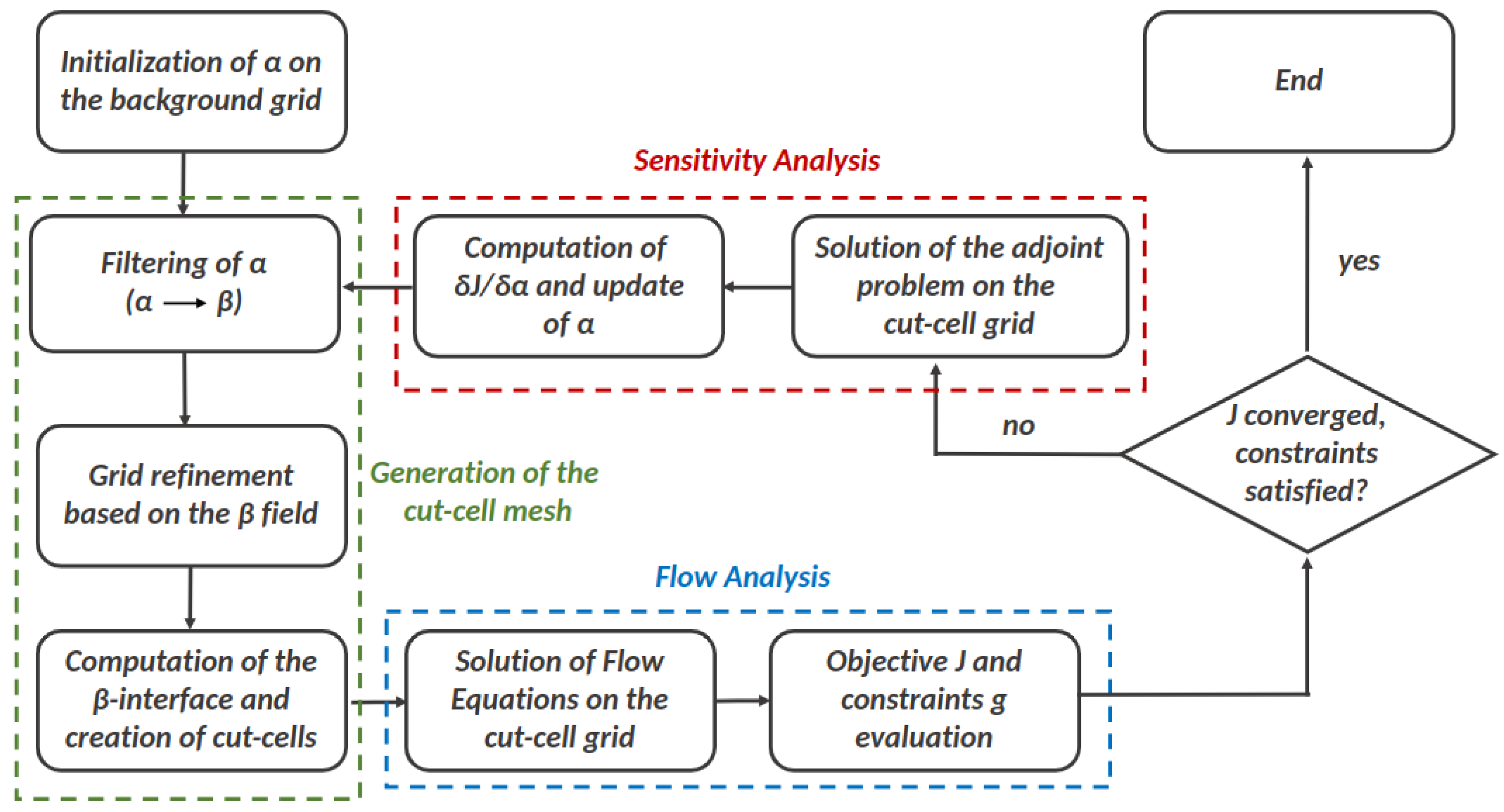By applying the chain rule of differentiation, these are transformed into derivatives with respect to the design variables $\alpha$ to be used to update the latter using the Method of Moving Asymptotes (MMA) [39]. The MMA creates and solves a convex optimization sub-problem in each TopO cycle, by creating convex approximations to the objective and constraint functions based on their computed gradients. The various steps of the TopO algorithm are presented schematically in Figure 1 and are further analyzed below.

2.1. Filtering of the Design Variables

To avoid grid-dependent solutions and eliminate the well-known checkerboard pathologies [40], a filtering scheme for the $\alpha$ field is utilized. This computes an auxiliary smoothed density field, $\beta$, by solving a Helmoltz-type filter PDE [41],

$$R^F\left(\beta ,\alpha \right)=-{\left(\frac{r}{2\sqrt{3}}\right)}^2\frac{{\partial }^2\beta }{\partial x_j^2}+\beta -\alpha =0$$

(1)

where $R^F\left(\beta ,\alpha \right)$ denotes the filtering operation and r is the radius, usually defined as 5 to 10 times the average edge length in the background grid. In addition, the usage of filtering “broadens” the effect of the design variables on the computed FSI and accelerates the convergence of the TopO.

2.2. Grid Refinement

In each optimization cycle, the grid close to the FSI is adequately refined in order to accurately simulate the flow and thermal boundary layers. Cells in the vicinity of the FSI are refined using an h-adaptivity approach. In what follows, the cells of the coarse grid to be refined are referred to as “parent” cells, whereas those resulting from the splitting of the “parent” cells are the “offspring”. Note that this work exclusively makes use of block-structured grids consisting purely of hexahedral cells (square elements of the same size/area in 2D).

In the beginning of this step, all background grid cells are set to have a uniform refinement level ($L_0$). Then, cells with $\beta$ values in the user-defined $[{\beta }_{min},{\beta }_{max}]$ range are selected for refinement. This range defines the bandwidths of cells close to the FSI to be refined, even though the $\beta$ field is not a distance field. ${\beta }_{min}=0.3$ and ${\beta }_{max}=0.7$ are used in the examples presented here in order to refine the cells in a broad band across the FSI. Then, cells are added to or subtracted from the previously selected set in order to meet the grid regularity requirements. In particular, cells are marked or unmarked for refinement in such a way that keeps the level difference of adjacent cells equal to 1, at most; this is imposed for stability reasons. The cells to be refined are split into 4 (in 2D) or 8 (in 3D) offspring cells, each having a refinement level of $L_P+1$, where $L_P$ is the level of their parent cell. An octree (in 3D) or quadtree (in 2D) data structure is used to store the information regarding parent and offspring cells. The cell selection and refinement process described above is repeated several times in each optimization cycle, until a user-defined maximum refinement level $L_{max}$ is reached. 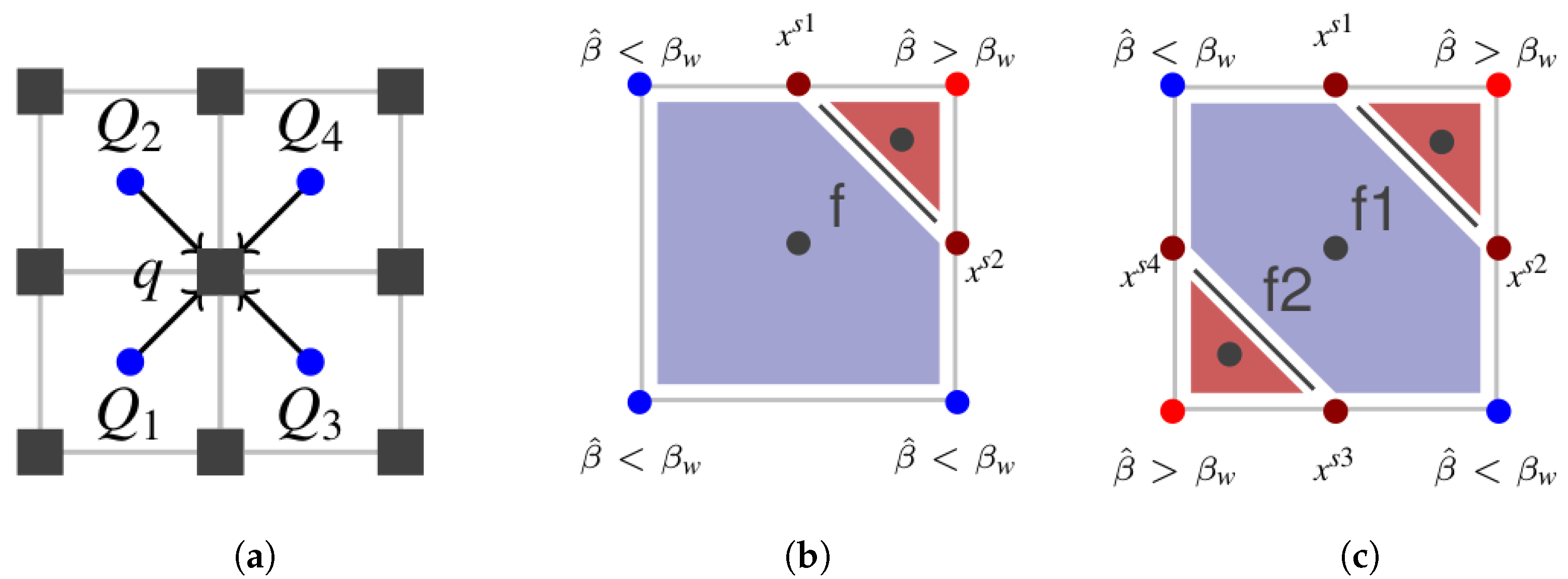At the end of each refinement step, the $\beta$ field is interpolated to the offspring cells, and the selection criterion for new refinement cells is applied again. In this work, a trilinear polynomial of the following form

$$\beta \left(x,y,z\right)={\overrightarrow{p}}^T·\overrightarrow{c}=\left[1,x,y,z,xy,xz,yz,xyz\right]·{\left[c_0,c_1,c_2,c_3,c_4,c_5,c_6,c_7\right]}^T$$

(2)

is constructed for each refined parent cell in terms of the coordinates $(x,y,z)$ in the local coordinate system and is used to compute the $\beta$ values at the offspring cell centers. At each vertex i of the parent cell, ${\widehat{\beta }}_i={\overrightarrow{p}}_i^T·\overrightarrow{c}$ should hold. Here, ${\widehat{\beta }}_i$ denotes the interpolated $\beta$ value from adjacent cells to vertex i. In a grid with hexahedra, this leads to the formation of an $8\times 8$ linear system of equations of the form $A·\overrightarrow{c}=\overrightarrow{\widehat{\beta }}$. By inverting A, the unknown coefficients can be expressed as a linear combination of ${\widehat{\beta }}_i$, i.e., $c_i={\alpha }_{ij}{\widehat{\beta }}_j$, and Equation (2) can be written as

$$\beta \left(x,y,z\right)={\overrightarrow{p}}^T·A^{-1}·\overrightarrow{\widehat{\beta }}$$

(3)

Equation (3) requires the $\widehat{\beta }$ values at grid vertices prior to the refinement. These are computed by interpolating $\beta$ from cells to vertices, according to

$${\widehat{\beta }}_p=\frac{{\sum }_{C\in Cells\left(p\right)}{\omega }_{pC}{\beta }_C}{{\sum }_{C\in Cells\left(p\right)}{\omega }_{pC}}$$

(4)

where $Cells\left(p\right)$ is the set of cells sharing vertex p and ${\omega }_{pC}=\frac{1}{\parallel x_i^p-x_i^C\parallel }$ are inverse-distance interpolation weights. Differentiating Equation (4) with respect to $\beta$ at any cell Q yields

$$\frac{\delta {\widehat{\beta }}_p}{\delta {\beta }_Q}=\frac{{\omega }_{pQ}}{{\sum }_{C\in Cells\left(p\right)}{\omega }_{pC}}$$

(5)

if Q belongs on the list of cells sharing p as a vertex, or 0 otherwise. This will later be used as part of the chain rule to compute ${\displaystyle \frac{\delta \mathcal{J}}{\delta \alpha }}$.

2.3. Generation of Cut Cells

The $\beta$ field, interpolated at the refined grid vertices though Equation (4), is used to compute the FSI and create body-fitted grids at each optimization cycle. The FSI reflects the intersection of grid edges by the ${\beta }_w=0.5$ iso-surface (or isoline in 2D). An edge connecting nodes A and B with values ${\widehat{\beta }}_A<{\beta }_w<{\widehat{\beta }}_B$ is intersected at

$$x_i^S=x_i^A+\frac{{\beta }_w-{\widehat{\beta }}_A}{{\widehat{\beta }}_B-{\widehat{\beta }}_A}\left(x_i^B-x_i^A\right)$$

(6)

Based on Equation (6), the derivative of $x_i^S$ with respect to $\widehat{\beta }$ at any node M is computed as

$$\frac{\delta x_i^S}{\delta {\widehat{\beta }}_M}=\frac{x_i^B-x_i^A}{{\widehat{\beta }}_B-{\widehat{\beta }}_A}\left(\frac{{\beta }_w-{\widehat{\beta }}_B}{{\widehat{\beta }}_B-{\widehat{\beta }}_A}{\delta }_A^M+\frac{{\widehat{\beta }}_A-{\beta }_w}{{\widehat{\beta }}_B-{\widehat{\beta }}_A}{\delta }_B^M\right)$$

(7)

where $\delta$ is the Kronecker delta. Equation (7) is also part of the chain rule computing ${\displaystyle \frac{\delta \mathcal{J}}{\delta \alpha }}$.

Cut cells are created by connecting the computed nodes along the edges intersected by the iso-surface to define new internal grid faces. The node connectivity is computed as in [42,43]. The new internal faces split the initial cells into sub-cells belonging to ${\mathrm{\Omega }}_F$ and ${\mathrm{\Omega }}_S$. This is shown schematically in Figure 2, where the introduced internal faces correspond to the dark-gray edges. In practice, a cell might be intersected more than once by the ${\beta }_w$ iso-surface; see Figure 2c. Surface areas, centers, and normals for the newly added faces are computed using the $x_i^S$ coordinates. The same quantities are re-computed for intersected faces belonging to ${\mathrm{\Omega }}_F$ or ${\mathrm{\Omega }}_S$ using the defined $x_i^S$ nodes on these faces and the nodes of the background face with $\widehat{\beta }<{\beta }_w$ or $\widehat{\beta }>{\beta }_w$, respectively. Finally, the cell centers and volumes of the so-formed cut cells are computed.

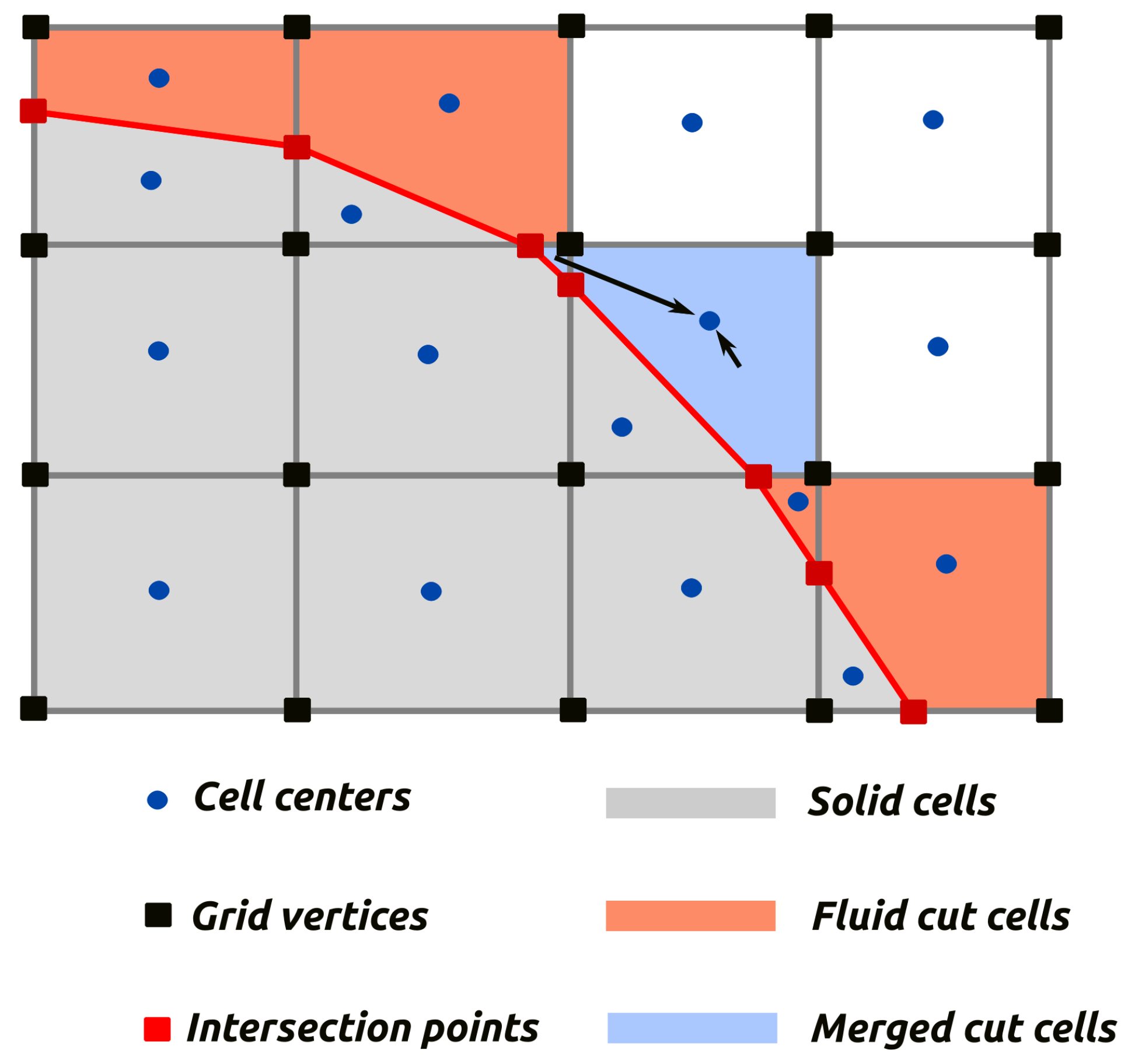
In practice, cut cells of small size can be generated. Their presence next to cells of much larger size might cause numerical instabilities during the flow solution, leading to convergence issues. To deal with this, each small cell is merged with a neighboring larger cell if its volume is less than $1\%$ of that of the latter [44], as shown in Figure 3. More than one small cell can be merged with the same neighboring cell, by also updating the grid connectivity information. Further discussion of this matter is beyond the scope of this work and can be found in many papers on conventional cut-cell methods [45,46,47].

Compared to level-set-based methods [48], the approach proposed here to track the FSI is simpler, since it avoids the re-initialization of the signed distance field in each optimization cycle by solving, for instance, the Hamilton Jacobi equation. Since the solution of the flow (see Section 2.4) and adjoint (see Section 2.6) equations takes place only in ${\mathrm{\Omega }}_F$, by discarding all cells belonging to ${\mathrm{\Omega }}_S$, the computational burden is reduced compared to that in standard density-based TopO. In other words, the systems of equations emerging from the discretization of the governing PDEs have as many cells as those in ${\mathrm{\Omega }}_F$, with the exception of the temperature equation, which is solved simultaneously in both ${\mathrm{\Omega }}_F$ and ${\mathrm{\Omega }}_S$, i.e., over the entire domain ${\mathrm{\Omega }}_d$.

2.4. Governing Equations

The governing equations for the flow and CHT problem are presented; their boundary conditions are summarized in Appendix A along with those of the adjoint problem. The flow solver (and its adjoint) is implemented in the in-house adjointOptimisation library [49] of OpenFOAM; the latter utilizes a finite-volume discretization and a cell-centered storage strategy. Details regarding the numerical solution of the governing PDEs follow.

2.4.1. Flow Equations

The flow is governed by the Navier–Stokes equations for incompressible fluids, which, in residual form, are written as

$$\begin{array}{cc}\hfill R^p& =\frac{\partial v_j}{\partial x_j}=0\hfill \end{array}$$

(8)

$$\begin{array}{cc}\hfill R_i^v& =v_j\frac{\partial v_i}{\partial x_j}+\frac{\partial p}{\partial x_i}-\frac{\partial {\tau }_{ij}}{\partial x_j}=0,i=1,2\hfill \end{array}$$

(9)

where p is the pressure divided by the constant fluid density and $v_i$ is the velocity. ${\tau }_{ij}=\left(\nu +{\nu }_t\right)\left(\frac{\partial v_i}{\partial x_j}+\frac{\partial v_j}{\partial x_i}\right)$ is the stress tensor, where $\nu$ is the bulk and ${\nu }_t$ the eddy viscosity. The later is modeled by the Spalart–Allmaras turbulence model [50] equation

$$R^{\tilde{\nu }}=v_j\frac{\partial \tilde{\nu }}{\partial x_j}-\frac{\partial }{\partial x_j}\left(\frac{\left(\nu +\tilde{\nu }\right)}{\sigma }\frac{\partial \tilde{\nu }}{\partial x_j}\right)-\frac{c_{b2}}{\sigma }{\left(\frac{\partial \tilde{\nu }}{\partial x_j}\right)}^2+\tilde{\nu }\left(D\left(\tilde{\nu },y\right)-P\left(\tilde{\nu },y\right)\right)=0$$

(10)

solved to compute $\tilde{\nu }$. In Equation (10), $P\left(\tilde{\nu },y\right)=c_{b1}\tilde{S}$ and $D\left(\tilde{\nu },y\right)=c_{w1}{f}_w\frac{\tilde{\nu }}{y^2}$ are the production and dissipation terms of the model, respectively. The turbulence model functions are given by

$$\begin{array}{cc}\hfill \chi & =\frac{\tilde{\nu }}{\nu },f_{v1}=\frac{{\chi }^3}{{\chi }^3+c_{v1}^3},f_{v2}=1-\frac{\chi }{1+\chi f_{v1}},\tilde{S}=S+\frac{f_{v2}\tilde{\nu }}{{\kappa }^2{y}^2},S=\sqrt{2}\parallel \frac{1}{2}\left(\frac{\partial v_j}{\partial x_i}-\frac{\partial v_i}{\partial x_j}\right)\parallel \hfill \\ \hfill f_w& =g{\left[\frac{1+c_{w3}^6}{g^6+c_{w3}^6}\right]}^{\frac{1}{6}},g=r+c_{w2}\left(r^6-r\right),r=\frac{\tilde{\nu }}{\tilde{S}{\kappa }^2{y}^2}\hfill \end{array}$$

and its constants are $c_{b1}=0.1355$, $c_{b2}=0.622$, $\sigma =2/3$, $\kappa =0.41$, $c_{w1}=\frac{c_{b1}}{{\kappa }^2}+\frac{1+c_{b2}}{\sigma }$, $c_{w2}=0.3$, $c_{w3}=2$, and $c_{v1}=7.1$. Finally, the eddy viscosity is computed as ${\nu }_t=f_{v1}\tilde{\nu }$. To avoid extreme grid stretching close to the wall, the wall function technique, as in Spalding’s formula [51], is used.

The distances y from the nearest wall, including the FSI, are computed via the solution of the Hamilton–Jacobi equation [52], reading

$$R^y=\frac{\partial }{\partial x_j}\left(\frac{\partial y}{\partial x_j}y\right)-\left(1+ϵ\right)y\frac{{\partial }^{2}y}{\partial x_j^2}-1=0$$

(11)

in which the diffusion term has been multiplied by $\left(1+ϵ\right)$, with $ϵ=0.1$, for stability reasons.

Equations (8)–(10) are solved in a segregated manner based on the Semi-Implicit Method for Pressure-Linked Equations (SIMPLE) [53], to handle the pressure–velocity coupling. Second-order upwind schemes are used to discretize the convection terms. Second-order central schemes are used for Laplace terms, using an explicit correction term to take into account the grid’s non-orthogonality. Finally, gradients are computed by applying Gauss’ theorem over control volumes; linear interpolation from cell to face centers is used to evaluate the field’s values at their boundaries.

2.4.2. Temperature Equation

The temperature field in ${\mathrm{\Omega }}_F$ is modeled by the advection–diffusion equation,

$$R_F^T={\rho }^F{c}_p^F{v}_j\frac{\partial T}{\partial x_j}-\frac{\partial }{\partial x_j}\left(k_{eff}\frac{\partial T}{\partial x_j}\right)-Q=0$$

(12)

Here, ${\rho }^F$ is the fluid density, and $c_p^F$ is the fluid-specific heat capacity. $k_{eff}=k_F+k_t$ is the effective thermal conductivity, which includes a laminar $k_F$ and a turbulent ${\displaystyle k_t=\frac{{\rho }^F{c}_p^F{\nu }_t}{P{r}_t}}$ part, where $P{r}_t$ is the turbulent Prandtl number. The assumption that the fluid’s thermophysical properties do not depend on the temperature is made. In Equation (12), Q is a volumetric heat source term that can be either constant or given in the form of $h\left(T_{ref}-T\right)$, where h is a constant heat transfer coefficient and $T_{ref}$ a reference temperature. This difference in the form of Q (and the corresponding physics) is the main distinction between the two cases presented in Section 4.

In ${\mathrm{\Omega }}_S$, heat conduction ($R_S^T=0$) is modeled by the same equation, by replacing $k_{eff}$ with $k_S$ (solid thermal conductivity), while considering zero velocity, guaranteed by the exact boundary conditions over the FSI, due to the use of cut cells.

The discretization of Equation (12) using finite volumes assumes integration over the boundaries of each cell, which requires $k_{eff}^f$ ($f=face$) to be available at the grid faces. For the internal faces of ${\mathrm{\Omega }}_F$ and ${\mathrm{\Omega }}_S$, the linear interpolation of $k_{eff}$ from cells to faces is used. However, special treatment is required at the FSI to accurately compute the diffusive fluxes $q^f$. There, the heat flux conservation property implies that $q^f=-q_F^f=q_S^f$, where $q_F^f$, $q_S^f$ are the outgoing heat fluxes from the fluid and solid parts. In discrete form,

$$q^f=-\underset{q_F^f}{\underbrace{\left(k_F+k_t^f\right)\frac{T^f-T^F}{{\Delta }^{Ff}}}}=\underset{q_S^f}{\underbrace{k_S\frac{T^f-T^S}{{\Delta }^{Sf}}}}$$

(13)

where $T^f$ is the temperature at the FSI; $T^F$, $T^S$ denote the temperature values at the adjacent fluid and solid cell centers, respectively; and ${\Delta }^{Ff}$, ${\Delta }^{Sf}$ are the distances of the cell centers in ${\mathrm{\Omega }}_F$ and ${\mathrm{\Omega }}_S$, adjacent to the FSI, from the latter. By solving Equation (13) for $T^f$ and substituting it back to either $q_F^f$ or $q_S^f$, the heat flux at the interface can be written in terms of $T^F$ and $T^S$ as

$$q^f=\underset{{\widehat{k}}_{eff}^f}{\underbrace{\frac{\left(k_F+k_t^f\right)k_s{\Delta }^{FS}}{\left(k_F+k_t^f\right){\Delta }^{Sf}+k_s{\Delta }^{Ff}}}}\frac{T^S-T^F}{{\Delta }^{FS}}$$

(14)

Equation (14) is consistent with the way in which the boundary conditions are imposed at the interface between adjacent domains in CHT simulations based on a partitioned approach [54].

2.5. Objective Functions and Constraints

In this work, TopO is applied to improve the performance of cooling devices. In the presented examples (see Section 4), a volumetric heat source term Q is applied over ${\mathrm{\Omega }}_S$ and this causes the T over the solid to increase. Due to the high thermal conductivity of the solid material, the applied heat is then transferred to the fluid/coolant and is removed through the domain outlet. Depending on the way in which heat is provided to the system, the TopO aims either to minimize the average temperature

$${\mathcal{J}}_T=\frac{{\int }_{{\mathrm{\Omega }}_S}Td\mathrm{\Omega }}{{\int }_{{\mathrm{\Omega }}_S}d\mathrm{\Omega }}$$

(15)

over ${\mathrm{\Omega }}_S$ or to maximize the amount of heat transferred from the solid to the fluid. The latter is the difference in the convecting energy fluxes evaluated at the inlet ($S_I$) and the outlet ($S_O$), i.e.,

$${\mathcal{J}}_H={\int }_{S_I}{\rho }^F{c}_p^F{v}_j{n}_{j}TdS+{\int }_{S_O}{\rho }^F{c}_p^F{v}_j{n}_{j}TdS$$

(16)

Note that, due to the way in which the normal vectors are defined, the two integrals on the right-hand side of Equation (16) have opposite signs.

An increase in cooling performance usually comes at the expense of higher power consumption in order to maintain the flow. The energy loss due to friction forces at the solid walls is given by the volume flowrate–weighted total pressure ($p_t=p+\frac{1}{2}{v}_k^2$) drop between the inlet and outlet,

$${\mathcal{P}}_L=-{\int }_{S_I}{v}_j{n}_j{p}_{t}dS-{\int }_{S_O}{v}_j{n}_j{p}_{t}dS$$

(17)

which should not exceed a threshold value. This constraint is expressed as

$$g_{{\mathcal{P}}_L}=\frac{{\mathcal{P}}_L}{{\mathcal{P}}_L^0}-{\pi }_{{\mathcal{P}}_L}\le 0$$

(18)

where ${\mathcal{P}}_L^0$ is the power dissipation computed for the starting geometry of the TopO and ${\pi }_{{\mathcal{P}}_L}$ is the percentage value of the threshold. A second inequality constraint is imposed on the fluid volume so as not to exceed a target percentage (${\pi }_V$) of the analysis domain (${\mathrm{\Omega }}_d$) volume, as follows:

$$g_V=\frac{{\int }_{{\mathrm{\Omega }}_F}d\mathrm{\Omega }}{{\int }_{{\mathrm{\Omega }}_d}d\mathrm{\Omega }}-{\pi }_V\le 0$$

(19)

2.6. Continuous Adjoint Method for Sensitivity Analysis

To update the design variables $\alpha$ in each optimization cycle, the derivatives of the objective and the constraint functions with respect to $\alpha$ are computed using the continuous adjoint [10]. The formulation of the adjoint problem for a general objective function or constraint, $\mathcal{F}$, starts by augmenting it with the field integrals of the governing equations multiplied by the adjoint variables to form the Lagrangian, $Ł\left(\equiv \mathcal{F}\right)$, i.e.,

$$Ł=\mathcal{F}+{\int }_{{\mathrm{\Omega }}_F}\left(q{R}^p+u_i{R}_i^v+\widetilde{{\nu }_a}{R}^{\tilde{\nu }}+y_{\alpha }{R}^y\right)d\mathrm{\Omega }+{\int }_{{\mathrm{\Omega }}_d}{T}_{\alpha }{R}_{F,S}^{T}d\mathrm{\Omega }$$

(20)

where q is the adjoint pressure, $u_i$ is the adjoint velocity, $\widetilde{{\nu }_a}$ is the adjoint turbulence variable, $y_{\alpha }$ is the adjoint distance, and $T_{\alpha }$ is the adjoint temperature.

To compute the total variation in $\mathcal{F}$ due to changes in the shape of the interface, $Ł$ is differentiated with respect to the coordinates $x_m^s$ of the points on the FSI, with $\frac{\delta Ł}{\delta x_m^s}=\frac{\delta \mathcal{F}}{\delta x_m^s}$. Following the terminology used in shape optimization, these derivatives practically stand for the sensitivity map of $\mathcal{F}$ [55] on the FSI computed by the cut-cell method. Since the coordinates $x_m^s$ depend on the cell center $\beta \left(\alpha \right)$ values, the chain rule of differentiation is applied to compute the derivatives of $\mathcal{F}$ with respect to $\alpha$.

To derive the adjoint equations and their boundary conditions, $\frac{\delta Ł}{\delta x_m^s}$ is expanded using Gauss’ theorem and the identity $\frac{\delta }{\delta x_m^s}\left(\frac{\partial \mathrm{\Phi }}{\partial x_j}\right)=\frac{\partial }{\partial x_j}\left(\frac{\delta \mathrm{\Phi }}{\delta x_m^s}\right)-\frac{\partial \mathrm{\Phi }}{\partial x_k}\frac{\partial }{\partial x_j}\left(\frac{\delta x_k}{\delta x_m^s}\right)$ [56], relating spatial derivatives to total derivatives with respect to $x_m^s$ and holds for any quantity $\mathrm{\Phi }$. This mathematical development for CHT problems (governed by Equations (8)–(12)) can be found in [57] (therein, however, for shape optimization) and is not repeated here in the interest of brevity. $\frac{\delta Ł}{\delta x_m^s}$ is written as

$$\begin{array}{cc}\hfill \frac{\delta Ł}{\delta x_m^s}& =\frac{\delta \mathcal{F}}{\delta x_m^s}+{\int }_{{\mathrm{\Omega }}_F}\left(R_i^u\frac{\delta v_i}{\delta x_m^s}+R^q\frac{\delta p}{\delta x_m^s}+R^{\widetilde{{\nu }_a}}\frac{\delta \tilde{\nu }}{\delta x_m^s}+R^{y_{\alpha }}\frac{\delta y}{\delta x_m^s}\right)d\mathrm{\Omega }+{\int }_{{\mathrm{\Omega }}_d}{R}_{F,S}^{T_{\alpha }}\frac{\delta T}{\delta x_m^s}d\mathrm{\Omega }\hfill \\ \hfill & +{\int }_{\partial {\mathrm{\Omega }}_F}\left(B{C}_i^u\frac{\delta v_i}{\delta x_m^s}+B{C}^q\frac{\delta p}{\delta x_m^s}+B{C}^{\widetilde{{\nu }_a}}\frac{\delta \tilde{\nu }}{\delta x_m^s}+B{C}^{y_{\alpha }}\frac{\delta y}{\delta x_m^s}+B{C}_F^{T_{\alpha }}\frac{\delta T}{\delta x_m^s}\right)dS-{\int }_{\partial {\mathrm{\Omega }}_F}{u}_i{n}_j\frac{\delta {\tau }_{ij}}{\delta b_n}dS\hfill \\ \hfill & -{\int }_{\partial {\mathrm{\Omega }}_F}\frac{\nu +\tilde{\nu }}{\sigma }\widetilde{{\nu }_a}\frac{\delta }{\delta b_n}\left(\frac{\partial \tilde{\nu }}{\partial x_j}{n}_j\right)dS+{\int }_{\partial {\mathrm{\Omega }}_F}\frac{\nu +\tilde{\nu }}{\sigma }\widetilde{{\nu }_a}\frac{\partial \tilde{\nu }}{\partial x_j}\frac{\delta n_j}{\delta b_n}dS-{\int }_{\partial {\mathrm{\Omega }}_F}{T}_{\alpha }\frac{\delta q_F}{\delta x_m^s}dS-{\int }_{\partial {\mathrm{\Omega }}_S}{T}_{\alpha }\frac{\delta q_S}{\delta x_m^s}dS\hfill \\ \hfill & +{\int }_{\partial {\mathrm{\Omega }}_S}B{C}_S^{T_{\alpha }}\frac{\delta T}{\delta x_m^s}dS+{\int }_{\partial {\mathrm{\Omega }}_F}{T}_{\alpha }\left(k_F+k_t\right)\frac{\partial T}{\partial x_j}\frac{\delta n_j}{\delta x_m^s}dS+{\int }_{\partial {\mathrm{\Omega }}_S}{T}_{\alpha }{k}_S\frac{\partial T}{\partial x_j}\frac{\delta n_j}{\delta x_m^s}dS\hfill \\ \hfill & -{\int }_{\partial {\mathrm{\Omega }}_F}{\mathrm{\Theta }}_{jk}^F{n}_j\frac{\delta x_k}{\delta x_m^s}dS+{\int }_{{\mathrm{\Omega }}_F}\frac{\partial {\mathrm{\Theta }}_{jk}^F}{\partial x_j}\frac{\delta x_k}{\delta x_m^s}d\mathrm{\Omega }-{\int }_{\partial {\mathrm{\Omega }}_S}{\mathrm{\Theta }}_{jk}^S{n}_j\frac{\delta x_k}{\delta x_m^s}dS+{\int }_{{\mathrm{\Omega }}_S}\frac{\partial {\mathrm{\Theta }}_{jk}^S}{\partial x_j}\frac{\delta x_k}{\delta x_m^s}d\mathrm{\Omega }\hfill \end{array}$$

(21)

The undefined terms in Equation (21) will become clear as the analysis proceeds.

To avoid the computation of $\frac{\delta v_i}{\delta x_m^s}$, $\frac{\delta p}{\delta x_m^s}$, $\frac{\delta \tilde{\nu }}{\delta x_m^s}$, $\frac{\delta y}{\delta x_m^s}$, $\frac{\delta T}{\delta x_m^s}$ in the fluid and solid domains, field integrals including them in Equation (21) are eliminated by setting their multipliers to zero, giving rise to the field adjoint equations

$$\begin{array}{cc}\hfill R^q& =\frac{\partial u_i}{\partial x_i}=0\hfill \end{array}$$

(22)

$$\begin{array}{cc}\hfill R_i^u& =-\frac{\partial \left(v_j{u}_i\right)}{\partial x_j}+u_j\frac{\partial v_j}{\partial x_i}+\frac{\partial q}{\partial x_i}-\frac{\partial {\tau }_{ij}^{\alpha }}{\partial x_j}+\frac{\partial }{\partial x_j}\left(\frac{C_{\tilde{S}}}{S}\widetilde{{\nu }_a}\tilde{\nu }\left(\frac{\partial v_i}{\partial x_j}-\frac{\partial v_j}{\partial x_i}\right)\right)\hfill \\ \hfill & +{\rho }^F{c}_p^F{T}_{\alpha }\frac{\partial T}{\partial x_i}+\frac{\partial \mathcal{F}}{\partial v_i}=0,i=1,2\hfill \end{array}$$

(23)

$$\begin{array}{cc}\hfill R^{\widetilde{{\nu }_a}}& =-\frac{\partial \left(v_j\widetilde{{\nu }_a}\right)}{\partial x_j}-\frac{\partial }{\partial x_j}\left(\frac{\nu +\tilde{\nu }}{\sigma }\frac{\partial \tilde{\nu }}{\partial x_j}\right)+\frac{1}{\sigma }\frac{\partial \tilde{\nu }}{\partial x_j}\frac{\partial \widetilde{{\nu }_a}}{\partial x_j}+2\frac{c_{b2}}{\sigma }\frac{\partial }{\partial x_j}\left(\widetilde{{\nu }_a}\frac{\partial \tilde{\nu }}{\partial x_j}\right)\hfill \\ \hfill & +\widetilde{{\nu }_a}\left(D\left(\tilde{\nu },y\right)-P\left(\tilde{\nu },y\right)\right)+C_{\tilde{\nu }}\tilde{\nu }\widetilde{{\nu }_a}+\frac{\partial u_i}{\partial x_j}\left(\frac{\partial v_i}{\partial x_j}+\frac{\partial v_j}{\partial x_i}\right)\frac{\delta {\nu }_t}{\delta \tilde{\nu }}+\frac{{\rho }^f{c}_p^F}{P{r}_t}\frac{\partial T_{\alpha }}{\partial x_j}\frac{\partial T}{\partial x_j}\frac{\delta {\nu }_t}{\delta \tilde{\nu }}+\frac{\partial \mathcal{F}}{\partial \tilde{\nu }}=0\hfill \end{array}$$

(24)

$$\begin{array}{cc}\hfill R^{y_{\alpha }}& =-2\frac{\partial }{\partial x_j}\left(\frac{\partial y}{\partial x_j}{y}_{\alpha }\right)-ϵy_{\alpha }\frac{{\partial }^{2}y}{\partial x_j^2}-ϵ\frac{\partial }{\partial x_j}\left(y\frac{\partial y_{\alpha }}{\partial x_j}\right)+C_y\tilde{\nu }\widetilde{{\nu }_a}=0\hfill \end{array}$$

(25)

$$\begin{array}{cc}\hfill R_F^{T_{\alpha }}& =-{\rho }^F{c}_p^F\frac{\partial \left(v_j{T}_{\alpha }\right)}{\partial x_j}-\frac{\partial }{\partial x_j}\left(k_{eff}\frac{\partial T_{\alpha }}{\partial x_j}\right)-Q_{\alpha }+\frac{\partial \mathcal{F}}{\partial T}=0\hfill \end{array}$$

(26)

where ${\tau }_{ij}^{\alpha }=\left(\nu +{\nu }_t\right)\left(\frac{\partial u_i}{\partial x_j}+\frac{\partial u_j}{\partial x_i}\right)$ is the adjoint stress tensor and $Q_{\alpha }$ is the adjoint heat source term. Terms $C_{\tilde{S}}$, $C_{\tilde{\nu }}$, and $C_y$ emerge from the differentiation of the production and dissipation terms in Equation (10) with respect to $\tilde{S}$, $\tilde{\nu }$, and y and can be found in [58]. Eliminating the same derivatives along the boundaries of ${\mathrm{\Omega }}_F$ and ${\mathrm{\Omega }}_S$ gives rise to the adjoint boundary conditions, summarized in Appendix A.

The solution of the adjoint problem (Equations (22)–(26)) starts by first solving the adjoint temperature equation (Equation (26)) over the entire ${\mathrm{\Omega }}_d$ to compute $T_{\alpha }$. Equation (14) is used to evaluate the adjoint thermal diffusive flux at the FSI, by replacing T with $T_{\alpha }$. Then, the adjoint mean flow (Equations (22) and (23)) and turbulence model (Equation (24)) PDEs are solved in a segregated manner. In this work, the discretization of the adjoint equations, described in Section 2.7, is consistent with the one used for the primal problem (as in the discrete adjoint), leading to the computation of accurate sensitivity derivatives.

After satisfying the field adjoint equations and their boundary conditions, the remaining terms in Equation (21) are the shape sensitivity derivatives along the FSI,

$$\begin{array}{cc}\hfill \frac{\delta \mathcal{F}}{\delta x_m^s}& =-{\int }_{\partial {\mathrm{\Omega }}_F}{\mathrm{\Theta }}_{jk}^F{n}_j\frac{\delta x_k}{\delta x_m^s}dS+{\int }_{{\mathrm{\Omega }}_F}\frac{\partial {\mathrm{\Theta }}_{jk}^F}{\partial x_j}\frac{\delta x_k}{\delta x_m^s}d\mathrm{\Omega }-{\int }_{\partial {\mathrm{\Omega }}_S}{\mathrm{\Theta }}_{jk}^S{n}_j\frac{\delta x_k}{\delta x_m^s}dS+{\int }_{{\mathrm{\Omega }}_S}\frac{\partial {\mathrm{\Theta }}_{jk}^S}{\partial x_j}\frac{\delta x_k}{\delta x_m^s}d\mathrm{\Omega }\hfill \\ \hfill & +{\int }_{\partial {\mathrm{\Omega }}_F}{u}_{〈n〉}{\tau }_{ij}\frac{\delta \left(n_i{n}_j\right)}{\delta x_m^s}dS+{\int }_{\partial {\mathrm{\Omega }}_F}\left(k_F+k_t\right)T_{\alpha }\frac{\partial T}{\partial x_j}\frac{\delta n_j}{\delta x_m^s}dS+{\int }_{\partial {\mathrm{\Omega }}_S}{k}_S{T}_{\alpha }\frac{\partial T}{\partial x_j}\frac{\delta n_j}{\delta x_m^s}dS\hfill \end{array}$$

(27)

where

$$\begin{array}{cc}\hfill {\mathrm{\Theta }}_{jk}^F& =q\frac{\partial v_j}{\partial x_k}-v_j{u}_i\frac{\partial v_i}{\partial x_k}-u_j\frac{\partial p}{\partial x_k}+u_i\frac{\partial {\tau }_{ij}}{\partial x_k}-{\tau }_{ij}^{\alpha }\frac{\partial v_i}{\partial x_k}\hfill \\ \hfill & -\widetilde{{\nu }_a}\left(v_j\frac{\partial \tilde{\nu }}{\partial x_k}-\frac{\partial }{\partial x_k}\left(\frac{\nu +\tilde{\nu }}{\sigma }\frac{\partial \tilde{\nu }}{\partial x_j}\right)-2\frac{c_{b2}}{\sigma }\frac{\partial \tilde{\nu }}{\partial x_j}\frac{\partial \tilde{\nu }}{\partial x_k}-\frac{C_{\tilde{S}}}{S}\tilde{\nu }\left(\frac{\partial v_i}{\partial x_j}+\frac{\partial v_j}{\partial x_i}\right)\frac{\partial v_i}{\partial x_k}\right)-\frac{\nu +\tilde{\nu }}{\sigma }\frac{\partial \widetilde{{\nu }_a}}{\partial x_j}\frac{\partial \tilde{\nu }}{\partial x_k}\hfill \\ \hfill & -2y_{\alpha }\frac{\partial y}{\partial x_j}\frac{\partial y}{\partial x_k}-T_{\alpha }\left({\rho }^F{c}_p^F{v}_j\frac{\partial T}{\partial x_k}-\frac{\partial }{\partial x_k}\left(\left(k_F+k_t\right)\frac{\partial T}{\partial x_j}\right)\right)-\left(k_F+k_t\right)\frac{\partial T_{\alpha }}{\partial x_j}\frac{\partial T}{\partial x_k}\hfill \end{array}$$

(28)

$$\begin{array}{cc}\hfill {\mathrm{\Theta }}_{jk}^S& =k_S{T}_{\alpha }\frac{{\partial }^{2}T}{\partial x_k\partial x_j}-k_S\frac{\partial T_{\alpha }}{\partial x_j}\frac{\partial T}{\partial x_k}\hfill \end{array}$$

(29)

Note that Equation (27) requires the grid sensitivities $\frac{\delta x_k}{\delta x_m^s}$ obtained by differentiating the coordinates of face centers along the FSI and the cut-cell centers with respect to $x_m^s$; the latter are given by closed-form expressions that can be found in [43].

Having computed ${\displaystyle \frac{\delta \mathcal{F}}{\delta x_m^s}}$, the chain rule of differentiation helps in computing ${\displaystyle \frac{\delta \mathcal{F}}{\delta \beta }}$ at cell P as

$$\frac{\delta \mathcal{F}}{\delta {\beta }_P}=\sum _{n=1}^{\mathcal{N}}\sum _{Q=1}^{NP}\frac{\delta \mathcal{F}}{\delta x_m^{sn}}\frac{\delta x_m^{sn}}{\delta {\widehat{\beta }}_Q}\frac{\delta {\widehat{\beta }}_Q}{\delta {\beta }_P}$$

(30)

where the first summation is over the $\mathcal{N}$ nodes along the FSI, whereas the second is over all $NP$ nodes at the edges cut by the FSI. The derivatives ${\displaystyle \frac{\delta x_m^{sn}}{\delta {\widehat{\beta }}_Q}}$, ${\displaystyle \frac{\delta {\widehat{\beta }}_Q}{\delta {\beta }_P}}$ are obtained through Equations (5) and (7), respectively. Using the proposed method, non-zero derivatives with respect to $\beta$ are computed only at cells close to the FSI. From this point of view, the proposed TopO method resembles level-set -based rather than the standard density-based TopO. As a final step, the filtering operation $R^F\left({\mathrm{\Psi }}^{\beta },\frac{\delta \mathcal{F}}{\delta \beta }\right)$ (see Section 2.1) is applied to $\frac{\delta \mathcal{F}}{\delta \beta }$ to yield the derivatives with respect to $\alpha$ at each cell P of the background mesh, viz. $\frac{\delta \mathcal{F}}{\delta {\alpha }_P}={\mathrm{\Psi }}_P^{\beta }{\mathrm{\Omega }}_P$, where ${\mathrm{\Omega }}_P$ is the cell volume.

2.7. “Think Discrete–Do Continuous” Adjoint Discretization

To compute the gradient of the discretized objective with respect to the design variables as accurately as in the discrete adjoint, the continuous adjoint PDEs (Equations (22)–(26)) should be discretized in a manner consistent with the primal equations. In this work, this is achieved by the “Think Discrete–Do Continuous” (TDDC) adjoint, firstly introduced by the present group of authors in [38] for use in aerodynamic shape optimization. It is now extended to TopO with CHT. The derivation of the TDDC adjoint starts from the derivation of a (hand-differentiated) discrete adjoint.

The method is exemplified through the derivation of the consistent discretization of the convection term in the adjoint temperature equation (Equation (26)), which emerges from the differentiation of term ${\rho }^F{c}_p^F{v}_j\frac{\partial T}{\partial x_j}$ (Equation (12)). Integrating the convection term of Equation (12) over the finite volume ${\mathrm{\Omega }}_P$, using the Gauss divergence theorem and a second-order upwind interpolation, yields

$$R_{F,P}^T=\sum _{f\in F\left(P\right)}\underset{{\mathrm{\Phi }}_{FO}^{T,PN}}{\underbrace{{\rho }^F{c}_p^F{v}_{〈n〉}^{PN}\left(w_U^{PN}{T}_P+{\tilde{w}}_U^{PN}{T}_N\right)\Delta S^f}}+\sum _{f\in F\left(P\right)}\underset{{\mathrm{\Phi }}_{SO}^{T,PN}}{\underbrace{{\rho }^F{c}_p^F{v}_{〈n〉}^{PN}\left(w_U^{PN}\frac{\partial T}{\partial x_j}{|}_P{d}_j^{Pf}+{\tilde{w}}_U^{PN}\frac{\partial T}{\partial x_j}{|}_N{d}_j^{Nf}\right)\Delta S^f}}$$

(31)

where $v_{〈n〉}^{PN}$ is the normal to the face f convecting velocity computed by the Rhie–Chow interpolation [59], $\Delta S^f$ are the face areas, and $w_U^{PN}$, ${\tilde{w}}_U^{PN}=1-w_U^{PN}$ are the upwind interpolation weights computed based on $v_{〈n〉}^{PN}$. Moreover, $d_j^{Pf}$ is the vector connecting the cell centroid to the face center. In Equation (31), summation is performed over the faces $F\left(P\right)$ of the finite volume. The spatial gradients of T are computed based on Gauss’ theorem and linear interpolation from cells to face centers, i.e.,

$$\frac{\partial T}{\partial x_j}{|}_P=\frac{1}{{\mathrm{\Omega }}_P}\sum _{f\in F\left(P\right)}\left(w_L^{PN}{T}_P+{\tilde{w}}_L^{PN}{T}_N\right)n_j^{PN}\Delta S^f$$

(32)

where $w_L^{PN}=\frac{|d_j^{Nf}|}{|d_j^{PN}|}$ are linear interpolation weights, computed using geometric distances. Here, ${\mathrm{\Phi }}_{FO}^{T,PN}$, ${\mathrm{\Phi }}_{SO}^{T,PN}$ denote the first- and second-order convecting fluxes at the faces.

The discrete form of the adjoint convection term $-{\rho }^F{c}_p^F\frac{\partial \left(v_j{T}_{\alpha }\right)}{\partial x_j}$ integrated over a control volume is

$$R_{F,P}^{T_{\alpha }}=-{\int }_{{\mathrm{\Omega }}_P}{\rho }^F{c}_p^F\frac{\partial \left(v_j{T}_{\alpha }\right)}{\partial x_j}d\mathrm{\Omega }=-\sum _{f\in F\left(P\right)}\left({\mathrm{\Phi }}_{FO}^{T_{\alpha },PN}+{\mathrm{\Phi }}_{SO}^{T_{\alpha },PN}\right)$$

(33)

where $FO$ and $SO$ have the same meaning as before. According to the proposed TDDC adjoint, the adjoint fluxes in Equation (33) should be computed as follows

$${\mathrm{\Phi }}_{FO}^{T_{\alpha },PN}={\rho }^F{c}_p^F{v}_{〈n〉}^f\left({\tilde{w}}_U^{PN}{T}_{\alpha P}+w_U^{PN}{T}_{\alpha N}\right)\Delta S^f,{\mathrm{\Phi }}_{SO}^{T_{\alpha },PN}={\rho }^F{c}_p^F\left({\tilde{w}}_L^{PN}\frac{\partial T_{\alpha }}{\partial x_j}{|}_P+w_L^{PN}\frac{\partial T_{\alpha }}{\partial x_j}{|}_N\right)n_j^{PN}\Delta S^f$$

(34)

for the discrete form of Equation (33) to be consistent with its primal counterpart (Equation (31)). The first-order adjoint flux in Equation (34) is similar to the corresponding first-order primal one, ${\mathrm{\Phi }}_{FO}^{TiPN}$, the only difference being that the upwind interpolation weights, $w_U^{PN}$, ${\tilde{w}}_U^{PN}$, have switched places. This suggests that a downwind scheme should be employed for the interpolation of $T_{\alpha }$ at the faces in conformity with the upwind propagating information in the adjoint problem. Additional differences can be seen in the second-order fluxes, in which the adjoint gradients are multiplied by the linear interpolation weights and are projected onto the face normal vectors, rather than the face-to-cell distance ones.

The spatial gradients in Equation (34) are discretized as follows

$$\frac{\partial T_{\alpha }}{\partial x_j}{|}_P{\mathrm{\Omega }}_P=-\sum _{f\in F\left(P\right)}{v}_{〈n〉}^{PN}\left({\tilde{w}}_U^{PN}{T}_{\alpha P}+w_U^{PN}{T}_{\alpha N}\right)d_j^{Pf}\Delta S^f+T_{\alpha P}\sum _{f\in F\left(P\right)}{v}_{〈n〉}^{PN}{d}_j^{Pf}\Delta S^f$$

(35)

where the fluxes in both terms are computed in a non-conservative manner (i.e., fluxes computed on the same face are different when seen from the two cells adjacent to that face, due to the presence of $d_j^{Pf}$). Despite this, the consistent second-order adjoint flux (Equation (34)) is conservative; this is in line with the fact that the adjoint energy equation (Equation (26)) is conservative too.

The full derivation of Equations (34) and (35) is given in Appendix B.

3. Comparison with Density-Based TopO (denTopO)

A sharp distinction between the proposed TopO workflow and that of the density-based approach (denTopO) is the ability of the former to apply proper boundary conditions along the FSI and generate (and adapt/refine) body-fitted grids. On the other hand, denTopO utilizes Brinkman penalization terms to simulate the effect that solidified areas have on the flow. These terms, expressed in terms of the material distribution field $\beta$, are added to Equations (9)–(11) (and their adjoints) and effectively treat solid walls as regions of high impermeability. For a flow variable $\varphi$, the corresponding Brinkman term is given by $B{S}^{\varphi }={\beta }_{max}I\left(\beta \right)\varphi$, where ${\beta }_{max}$ stands for the impermeability value of the solid material and takes high enough values to ensure that $\varphi \approx 0$ inside ${\mathrm{\Omega }}_S$. Its value is selected based on the non-dimensional Darcy number (set here to $Da={10}^{-5}$) expressing the ratio of viscous to porous forces as follows

$${\beta }_{max}=\frac{\nu }{Da·L^2}$$

(36)

where L is a characteristic length. $I\left(\beta \right)=\frac{\beta }{1+b_I\left(1-\beta \right)}$ is a convex function [7] and $b_I$ a steepening parameter, which penalizes intermediate density values, driving them closer to 0. In the examples of Section 4, whenever denTopO is utilized, $b_I=10$. The main disadvantage of this approach is that, in practice, the imposed penalization terms are not sufficient to impose exact zero values of the corresponding flow field inside ${\mathrm{\Omega }}_S$. For instance, for $\varphi =v_i$ in $B{S}^{\varphi }$, spurious unwanted flow leakage inside the solid areas, hindering the accuracy of the flow solution, usually occurs. Moreover, it does not support the use of the wall function technique in turbulent flows. To solve the CHT problem, the thermal conductivity k at the cell centers is interpolated between $k_F$ and $k_S$, using the $\beta$ field, as $k\left(\beta \right)=k_F+{\beta }^p\left(k_S-k_F\right)$, with $p=3$. The interpolation scheme used for k allows intermediate values to appear. Then, Equation (12) computes T over ${\mathrm{\Omega }}_d$ using $k_{eff}=k\left(\beta \right)+(1-\beta )k_t$ as the effective thermal conductivity. Note that denTopO is unable to accurately interpolate $k_{eff}$ at the FSI (Equation (14)), which is crucial in simulating heat transfer phenomena.

The second difference between cut-cell TopO and denTopO is related to the computation of the adjoint sensitivities with respect to $\alpha$. The cut-cell TopO is driven by shape sensitivities, which are, then, transformed into derivatives with respect to $\alpha$. These are used to update the design variables and, subsequently, the FSI’s position. Depending on the r value used in Equation (1), $\frac{\delta \mathcal{J}}{\delta \alpha }$ in cut-cell-based TopO takes on non-zero values at cells in the vicinity of the FSI. In denTopO, the derivative of $\mathcal{J}$ with respect to $\alpha$ at cell P is given by

$$\frac{\delta \mathcal{J}}{\delta {\alpha }_P}={\int }_{{\mathrm{\Omega }}_d}{\beta }_{max}\left(u_i{v}_i+\widetilde{{\nu }_a}\tilde{\nu }+y_{\alpha }y\right)\frac{\partial I\left(\beta \right)}{\partial \beta }\frac{\partial \beta }{\partial {\alpha }_P}d\mathrm{\Omega }+{\int }_{{\mathrm{\Omega }}_d}\frac{\partial T}{\partial x_j}\frac{\partial T_{\alpha }}{\partial x_j}\left[\left(k_S-k_F\right)p{\beta }^{p-1}-k_t\right]\frac{\partial \beta }{\partial {\alpha }_P}d\mathrm{\Omega }$$

(37)

These take on non-zero values everywhere in ${\mathrm{\Omega }}_d$, allowing thus more drastic topological changes between optimization cycles.

4. Application in CHT Problems

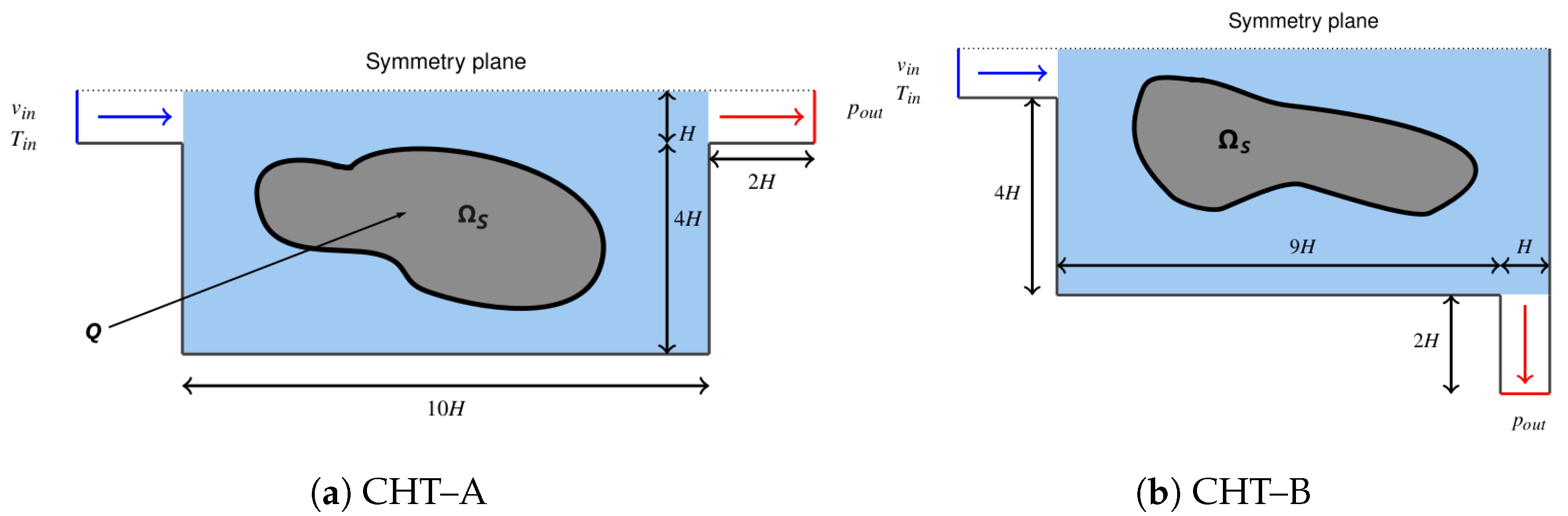
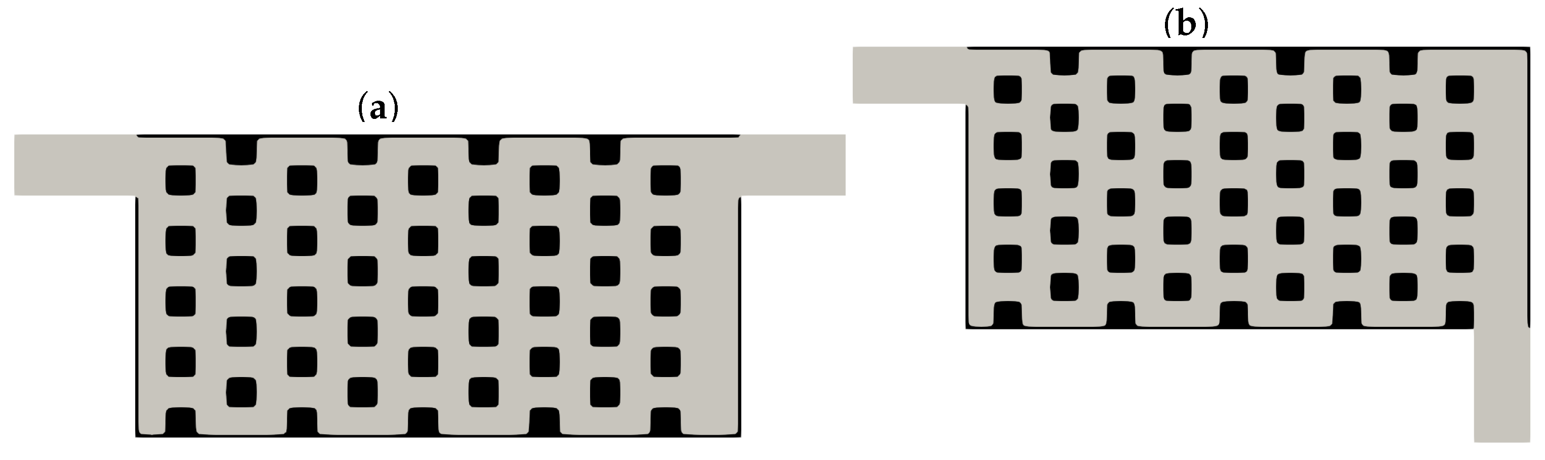
The proposed method is demonstrated in two different CHT TopO problems. The two topologies, having a single (CHT-A) and a split (CHT-B) outlet, can be found in Figure 4, with dimensions given in terms of the inlet height $H=0.1$ m. CHT-A was first defined in [19]. The design variables $\alpha$ take on a zero value inside the inlet and outlet channels (Figure 4) and are allowed to vary only in the central part of the geometry (shown in blue color in Figure 4; this stands for the design domain ${\mathrm{\Omega }}_D$), where a solid material (in gray color) can be added or subtracted. For both cases, a Cartesian background grid is generated, with $21.6$ K square cells of edge length equal to $h=\frac{H}{20}$. Even if both cases are symmetric with respect to the top horizontal line, the entire domain is shown in most figures presenting results.

The working fluid is air, with a constant density ${\rho }^F=1.18$ kg/m³, specific heat capacity $c_p^F=1004.9$ J/kg·K, thermal conductivity $k_F=0.0254$ W/m·K, and bulk viscosity $\nu =1.5\times {10}^{-5}$ m²/s. Moreover, $P{r}_t=1$. The solid material corresponds to aluminum with $k_S=237$ W/m·K. The fluid enters the domain at the temperature of $T_{in}=273$ K; the exit pressure is set to zero. The case Reynolds number is defined as $Re=\frac{v_{in}H}{\nu }$, in terms of the inlet velocity magnitude $v_{in}$. Unless specified otherwise, the inlet velocity is $v_{in}=0.375$ m/s, or $Re=2500$.

In CHT-A, the sought solid domain is heated by a constant volumetric heat source $Q=1$ kW/m². TopO seeks to minimize the average temperature over ${\mathrm{\Omega }}_S$ (${\mathcal{J}}_T$, Equation (15)). In CHT-B, the volumetric heat source term applied over ${\mathrm{\Omega }}_S$ is given by $Q=h\left(T_{ref}-T\right)$, where $h=10$ W/m²K and $T_{ref}=373$ K. Since Q is not fixed, the goal is to maximize the heat transferred to the coolant by maximizing ${\mathcal{J}}_H$ (Equation (16)). In both cases, the fluid volume (area in 2D) inside ${\mathrm{\Omega }}_D$ should be less than $45\%$ of ${\mathrm{\Omega }}_D$ (${\pi }_V\approx 0.49$ in Equation (19)). Power dissipation for CHT-A is controlled by setting ${\pi }_{{\mathcal{P}}_L}=0.33$ in Equation (18), whereas three different ${\pi }_{{\mathcal{P}}_L}$ values ($0.25$, $0.33$, and $0.5$) are used in CHT-B to investigate its effect on the cooling performance (see Section 4.4).

Regarding the MMA settings used in both cases, the adaptation parameters controlling the amount of the asymptote decrease or increase in each optimization cycle are set to $0.5$ and $1.05$, respectively, instead of the recommended (in [39]) values of $0.7$ and $1.2$. In addition, $\rho =5\times {10}^{-5}$ (as opposed to the default value of $1\times {10}^{-5}$) is used to increase the convexity of the approximated $\mathcal{J}$, $g_{{\mathcal{P}}_L}$, and $g_V$.

4.1. CHT-A Results Using denTopO

For the purpose of comparison, CHT-A is firstly optimized using the “standard” denTopO approach with Brinkman terms in the flow equations (see Section 2.4). Using the inlet height H as the characteristic length in Equation (36), ${\beta }_{max}=150$. As denTopO cannot trace the FSI, there is no clear boundary separating ${\mathrm{\Omega }}_F$ and ${\mathrm{\Omega }}_S$. Thus, ${\mathcal{J}}_T$ (Equation (15)) and $g_V$ (Equation (19)) are recast as follows

$${\mathcal{J}}_T=\frac{{\int }_{{\mathrm{\Omega }}_d}\beta Td\mathrm{\Omega }}{{\int }_{{\mathrm{\Omega }}_d}\beta d\mathrm{\Omega }},g_V=\frac{{\int }_{{\mathrm{\Omega }}_d}\left(1-\beta \right)d\mathrm{\Omega }}{{\int }_{{\mathrm{\Omega }}_d}d\mathrm{\Omega }}-{\pi }_V\le 0$$

(38)

where integrations over ${\mathrm{\Omega }}_d$ (instead of ${\mathrm{\Omega }}_F$ and ${\mathrm{\Omega }}_S$) are performed by considering the $\beta$ field. In addition, in Equation (12), the imposed heat source term Q is multiplied by $\beta$ to activate the term in the solidified part only. Note that, in this problem, as the solid volume changes during the optimization, the total amount of heat given to the solid, ${\int }_{{\mathrm{\Omega }}_d}\beta Qd\mathrm{\Omega }$, is not fixed. The volume constraint ensures that a minimum amount of heat is given to the system and avoids trivial all-fluid solutions.

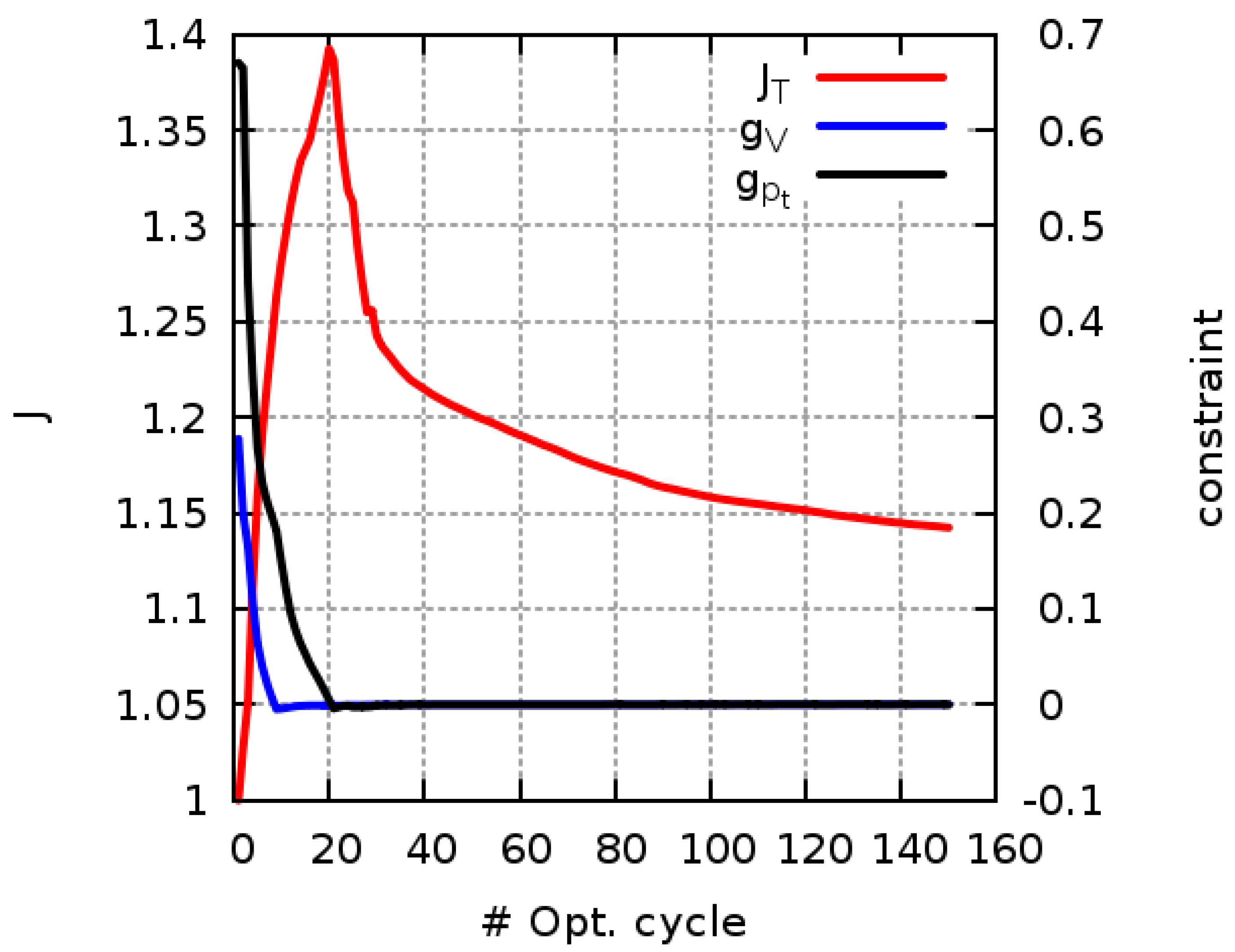
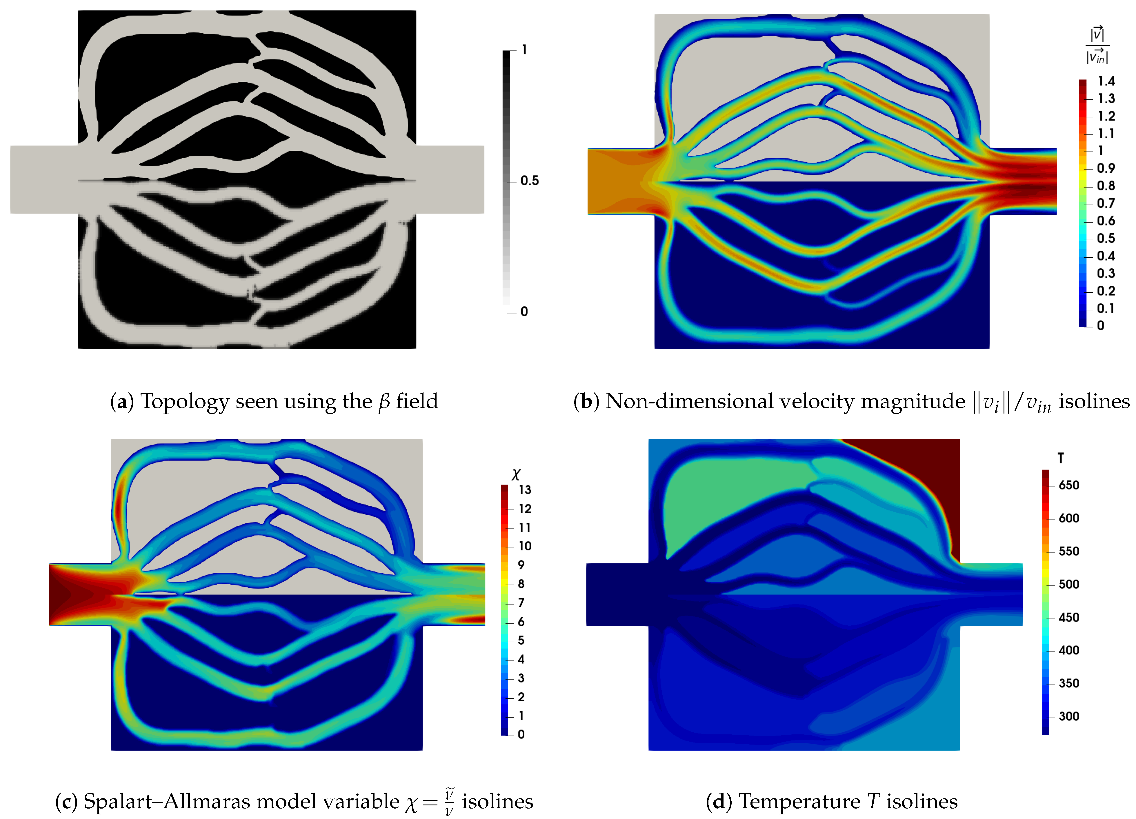
Figure 5 shows the convergence of the normalized ${\mathcal{J}}_T$ value and the imposed constraints. At the beginning of denTopO, both $g_V$ and $g_{{\mathcal{P}}_L}$ are violated. The first ∼$20$ cycles are spent to meet the inequality constraints; then, the MMA goes on to reduce ${\mathcal{J}}_T$ to $335.4$ K. The optimized distribution of $\beta$ is shown in the bottom half of Figure 6a. Even though the computed $\beta$ field in the optimized solution is almost binary, thin gray areas between the fluid and solid appear. The top half of Figure 6a corresponds to the optimized geometry, for which the FSI has been computed by post-processing the $\beta$ field to generate cut cells. On the background grid that is adapted to the FSI, the optimized solution is re-evaluated using the cut-cell code. This re-evaluation gives ${\mathcal{J}}_T=447.6$ K, with $g_{{\mathcal{P}}_L}=-0.14$. This means that, when re-evaluated with the cut-cell primal solver, the denTopO solution still has a lot of room before approaching the $P_L$ threshold, justifying the poor thermal performance. In terms of execution time, the cut-cell flow and adjoint solvers are ∼$38\%$ and ∼$30\%$ faster than the corresponding Brinkman solvers, for the same amount of SIMPLE iterations, without the usage of AMR, and on the same hardware. This reduction in computational cost is expected, considering that ${\mathrm{\Omega }}_S$ occupies ∼$51\%$ of ${\mathrm{\Omega }}_d$. Isolines for the non-dimensional velocity magnitude $\frac{\parallel v_i\parallel }{v_{in}}$, the intermediate Spalart–Allmaras model variable $\chi =\frac{\tilde{\nu }}{\nu }$, and the temperature T using the Brinkman and the cut-cell-based flow solvers are shown in Figure 6b–d, respectively. As indicated by the iso-velocity contours of Figure 6b, the re-evaluation on the cut-cell grid results in a different distribution of the incoming flow within the various channels. Due also to the inability of the denTopO flow solver to impose accurate boundary conditions on the FSI, significant discrepancies in the computed temperature fields between the two flow solvers can be seen, as in Figure 6d. This study highlights the importance of performing TopO based on solvers able to accurately compute physics. As shown in Section 4.3, a better-performing (in terms of cooling) design can be obtained using the proposed methodology.

4.2. Verification of Computed Sensitivities Using TDDC Adjoint

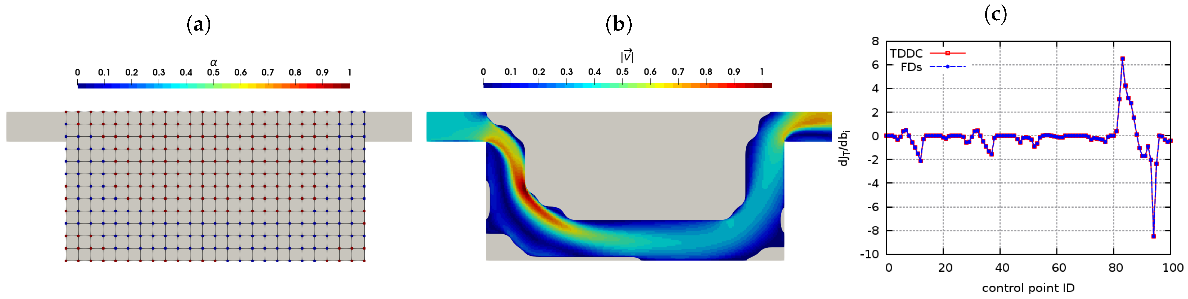
In this subsection, the computed sensitivity derivatives using the proposed TDDC adjoint of Section 2.7 are validated against finite differences (FDs) for CHT-A. To reduce the cost of the FDs, which depends directly on the number of design variables, a volumetric NURBS-based parameterization is used. In particular, a 2D lattice of $NX\times NY$ nodes controls the $\alpha$ values in cells lying within its boundaries; the latter coincide with the boundaries of ${\mathrm{\Omega }}_D$ (Figure 7). The ${\alpha }_{CP}$ values at the control points are the design variables of the problem, instead of the $\alpha$ values of the background grid cells. Since $NX=25$, $NY=13$, this leads to 325 design variables in total. A set of parametric coordinates ($u,v$) is assigned to each cell P, the center coordinates $(x_P,y_P)$ of which lie within the control lattice; the parametric coordinates at P are computed as $u_P=\frac{x_P-x_{min}}{x_{max}-x_{min}}$, $v_P=\frac{y_P-y_{min}}{y_{max}-y_{min}}$ and the $\alpha$ value as

$$a_P=\sum _{i=0}^{NX-1}\sum _{j=0}^{NY-1}{U}_i\left(u_P\right)V_j\left(v_P\right){\alpha }_{CP}^{ij}$$

(39)

where $U_i$, $V_j$ are the second-degree NURBS basis functions. Taking the derivative of Equation (39) with respect to ${\alpha }_{CP}^{lm}$ yields, $\frac{\delta {\alpha }_P}{\delta {\alpha }_{CP}^{lm}}=U_l\left(u_P\right)V_m\left(v_P\right)$.

The control lattice is shown in Figure 7a, whereas the resulting geometry after transforming the $\alpha$ field into cut cells is presented in Figure 7b; the velocity field is shown inside ${\mathrm{\Omega }}_F$, whereas ${\mathrm{\Omega }}_S$ is in gray. The derivatives of ${\mathcal{J}}_T$ with respect to the $\alpha$ cell values are computed by the adjoint method, as described in Section 2.6. The chain rule of differentiation transforms $\frac{\delta {\mathcal{J}}_T}{\delta {\alpha }_P}$ into $\frac{\delta {\mathcal{J}}_T}{\delta {\alpha }_{CP}^{lm}}$. The so-computed derivatives for the first 100 design variables are plotted in Figure 7c and are in perfect agreement with those computed by the FDs. This verifies the accuracy of the sensitivity derivatives of $\mathcal{J}$ when the TDDC adjoint discretization schemes are used. The same level of accuracy is obtained for the derivatives with respect to the remaining design variables, which are not shown here. It should be noted that the lattice shown in Figure 7 is used only in this comparison, to keep the cost of the FDs as low as possible, and not in any other study that follows.

4.3. CHT-A Results Using Cut-Cell-Based TopO

Having verified the accuracy of the computed derivatives using the TDDC adjoint, the latter is used by the cut-cell-based TopO to optimize the cooling in CHT-A. To initialize the case, ${\mathrm{\Omega }}_D$ has been seeded with multiple square solid structures of size $\frac{H}{2}$; see Figure 8a.

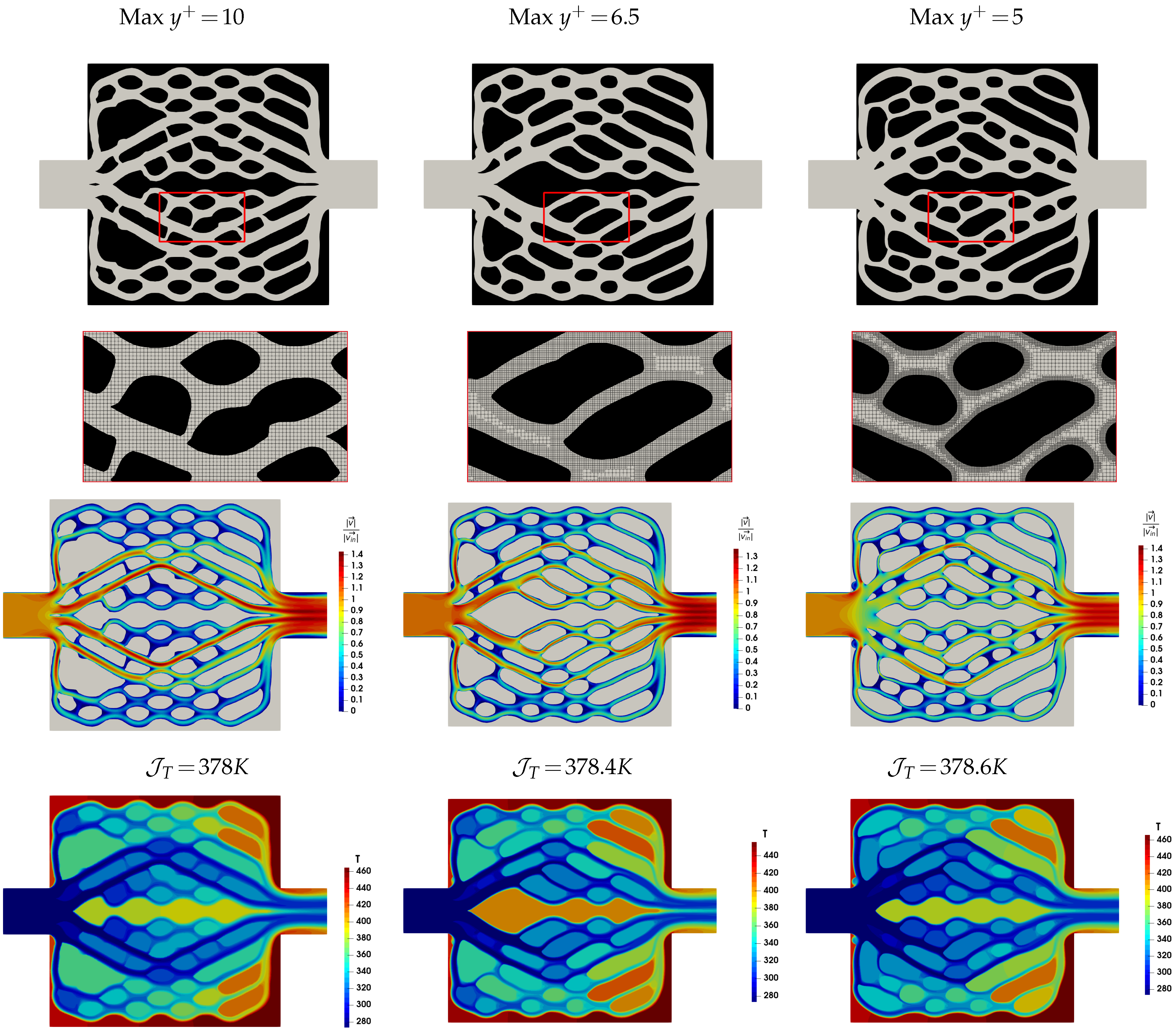
First, the importance of using the grid refinement strategy of Section 2.2 is demonstrated by solving the TopO problem with 0, 1, and 2 refinement steps. The three solutions will be referred to as R0, R1, and R2, respectively; see Figure 9. Small but significant differences exist among the three optimized geometries. Since the design variables of TopO are defined on the background grid, the unknown optimization variables are the same in all three cases; therefore, the differences in the optimized geometries can be attributed only to differences in the flow solution’s accuracy due to the grid refinement. At the end of the refinement process (if applied), the grid used to solve the flow consists of $21.6$ K, ∼$62$ K, and ∼$140$ K cells for R0, R1, and R2, respectively; a close-up view of the refined grid close to the FSI walls in the central area of the three optimized geometries is given in Figure 9. The maximum $y^{+}$ values computed at the cell centers adjacent to the FSI are also reported; as expected, lower values are computed as the grid resolution close to the FSI increases. According to the ${\mathcal{J}}_T$ values listed in Figure 9, each computed using the grid utilized during TopO, the three optimized designs perform equally well in terms of cooling. For a fair comparison, solutions R0 and R1 are re-evaluated after refining the background grid twice using the already optimized $\beta$ field. The computed ${\mathcal{J}}_T$ and $\Delta p_t$ values are listed in

Table 1. CHT-A: performance of solutions R0, R1 (both re-evaluated using two grid refinement steps), and R2. The power dissipation threshold value is $\Delta p_t^{thresh}={\rho }^F{\pi }_{{\mathcal{P}}_L}\Delta p_t^0=9.8\times {10}^{-2}$ Pa.

Solution	R0	R1	R2
$J_T\left[\mathrm{K}\right]$	$387.6$	$380.4$	$378.6$
$\Delta p_t\left[\times {10}^{-2}\mathrm{Pa}\right]$	$11.17$	$10.50$	$9.8$

. The power dissipation values of (the re-evaluated) R0 and R1 solutions exceed the maximum allowed value, which means that the $g_{{\mathcal{P}}_L}$ constraint is not met. Irrespective of the violation or not of this constraint, solution R2 outperforms R0 and R1 in terms of ${\mathcal{J}}_T$. The current study confirms the need to refine the grid during TopO.

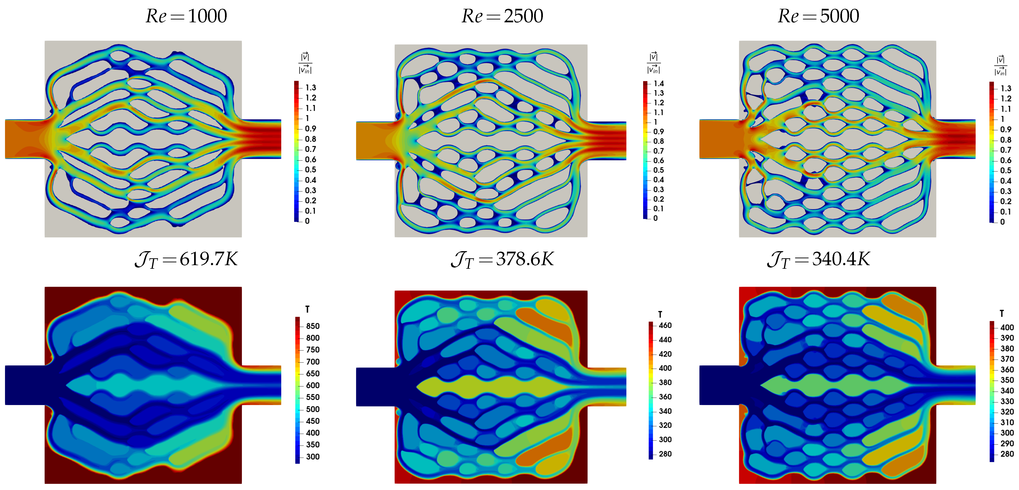
The Reynolds number’s effect on the optimized solution is also investigated. The optimization problem is solved for three different inlet velocity values, namely $v_{in}=0.15$ m/s, $0.375$ m/s, and $0.75$ m/s, corresponding to $Re=1000$, 2500, and 5000, respectively. Based on the previous study, the grid is refined twice in each cycle of TopO and this leads to the maximum $y^{+}$ values at cells adjacent to the FSI equal to 3, 5, and 8, respectively.

The optimized solutions for the three $Re$ are presented in Figure 10. The average temperature values in ${\mathrm{\Omega }}_S$ are also given. Note that the solution presented in the middle column of Figure 10 is identical to R2, as in Figure 9. The power dissipation value ${\mathcal{P}}_L^0$ of the initial design (Figure 8) increases as $Re$ increases and so does the maximum allowed power dissipation, according to Equation (18). In all optimized designs, a number of solid bodies, forming a network of flow channels inside the design domain for improved cooling, can be observed. For $Re=1000$, larger solid structures, aligned with the flow, are created. By increasing $Re$, more solid structures of smaller sizes, and thus more and narrower flow channels, are formed. Thus, the heat dissipation is enhanced and this is reflected in the average temperature values being equal to ${\mathcal{J}}_T=547.25$ K, 378 K, and $340.4$ K for $Re=1000$, 2500, and 5000, respectively. These observations are in agreement with those in [19,20]. 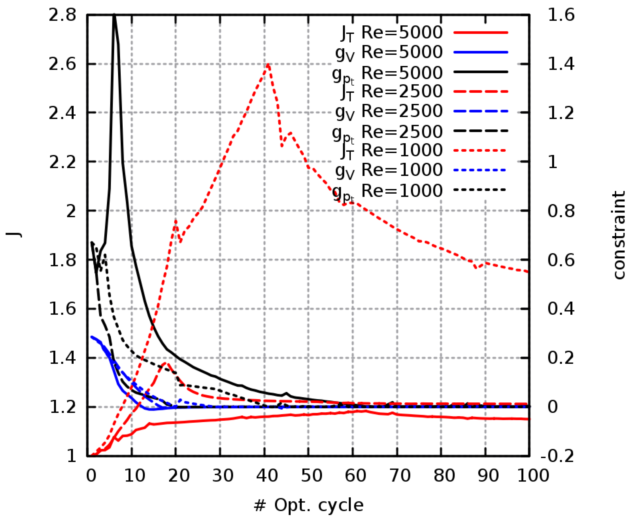Figure 11 shows the convergence of the normalized ${\mathcal{J}}_T$ value and of the imposed constraints for the three optimizations of Figure 10. In the beginning of the TopO, the fluid volume is more than $45\%$ of ${\mathrm{\Omega }}_D$ and, thus, $g_V$ is violated. As the solid material is added to meet $g_V$, more heat is given to the system and this leads to higher ${\mathcal{J}}_T$ values. Once $g_V$ has been satisfied, an almost constant amount of heat, $Q=275$ W, is imposed in all remaining cycles. After satisfying both $g_V$ and $g_{{\mathcal{P}}_L}$, the MMA tries to minimize the value of ${\mathcal{J}}_T$; see Figure 11. Since a further decrease in the fluid’s volume and $\Delta p_t$ would be counterproductive with respect to the cooling of CHT-A, both $g_V$ and $g_{{\mathcal{P}}_L}$ are practically satisfied as equality constraints ($g_V,g_{{\mathcal{P}}_L}\approx 0$).

4.4. CHT-B Results Using Cut-Cell-Based TopO

The ability of the proposed method to generate optimal topologies is demonstrated in a second configuration, in which the outlet duct has been re-located to the bottom right of ${\mathrm{\Omega }}_D$; see Figure 4b. Compared to CHT-A, the solid material is heated up according to the following volumetric heat source term: $Q=h\left(T_{ref}-T\right)$. TopO seeks to maximize the heat transferred to the fluid. The latter is expressed by ${\mathcal{J}}_H$ (Equation (16)), which, after taking into consideration the energy conservation, is equivalent to ${\int }_{{\mathrm{\Omega }}_S}h\left(T_{ref}-T\right)d\mathrm{\Omega }$. As in CHT-A, the initial design has been seeded with multiple square solid structures; see Figure 8b.

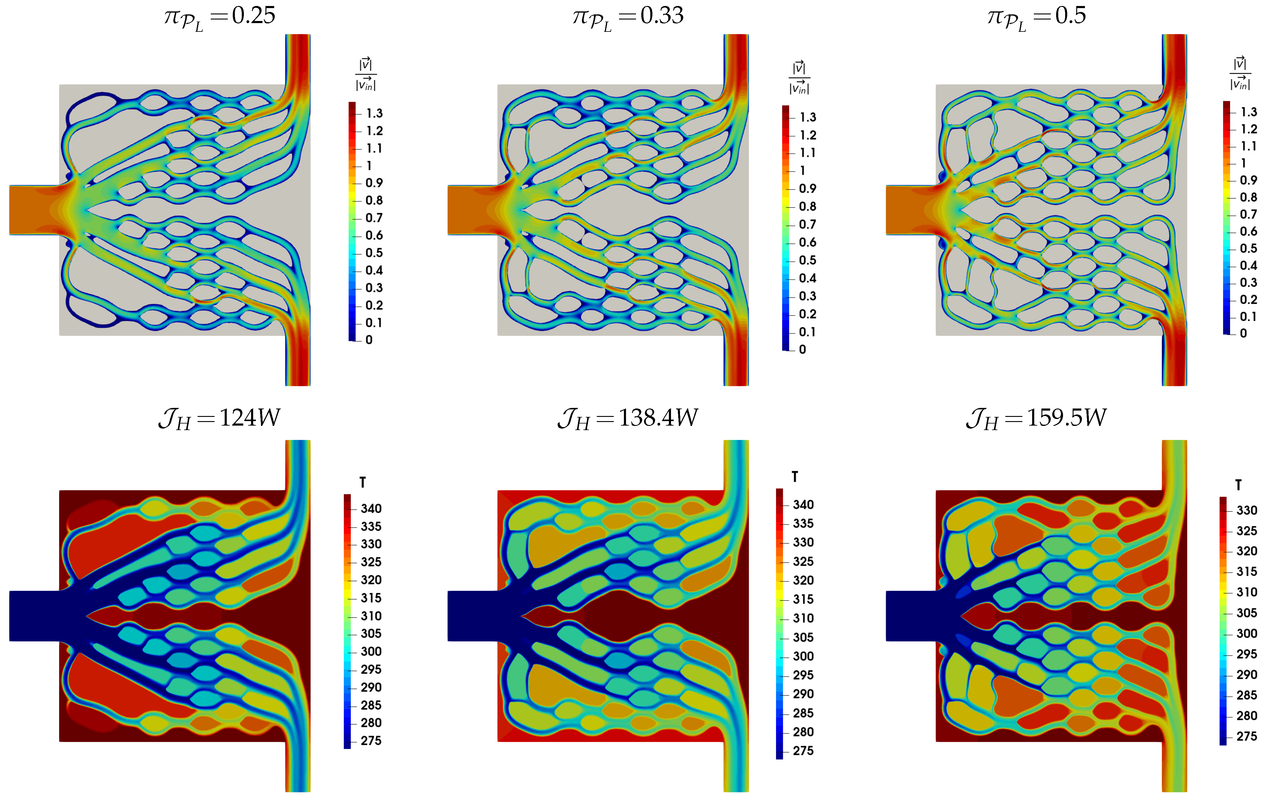
The influence of the maximum allowed power dissipation inside the heat exchanger is investigated by performing the optimization for three different ${\pi }_{{\mathcal{P}}_L}$ values (Equation (18)), namely ${\pi }_{{\mathcal{P}}_L}=0.25$, ${\pi }_{{\mathcal{P}}_L}=0.33$, and ${\pi }_{{\mathcal{P}}_L}=0.5$. The background grid is refined twice in each TopO cycle. The optimized solutions are presented in Figure 12. Increasing ${\pi }_{{\mathcal{P}}_L}$, and thus the allowed power dissipation, leads to the formation of more flow channels for enhanced heat transfer. The average temperature inside ${\mathrm{\Omega }}_S$ for the three designs shown in Figure 12 is ${\mathcal{J}}_T=327.9K$, $323.4K$, and $318.6K$. As expected, lower values of ${\mathcal{J}}_T$ are obtained by increasing ${\pi }_{{\mathcal{P}}_L}$ as this allows more heat to be exchanged.

5. Conclusions

A TopO framework that combines a material distribution field (design variables) and the cut-cell method to tackle laminar and turbulent flow problems with CHT is proposed. Here, the design variables are defined at the cell centers of a background grid and their post-processing yields an auxiliary field $\beta$ that helps to identify fluid and solid areas, as well as the FSI as the ${\beta }_w=0.5$ iso-surface. The FSI’s intersections with the background grid generate cut cells, giving rise to a body-fitted grid on which the flow equations are solved by applying proper boundary conditions, including wall functions. As cells belonging to ${\mathrm{\Omega }}_S$ are discarded, the solution cost of the flow and adjoint equations is reduced (by up to ∼$38\%$ in the examined cases). Additionally, the proposed workflow is able to locally refine the grid close to the FSI to capture the flow physics. The proposed method replaces the Brinkman penalization terms in the flow equations, frequently met in TopO, with the imposition of exact boundary conditions on the FSI and, thus, avoids spurious flow leakage inside ${\mathrm{\Omega }}_S$.

To facilitate TopO, the continuous adjoint method is derived for the CHT problem and computes the sensitivity map of $\mathcal{J}$ on the FSI. The chain rule is applied on the computed shape sensitivities, yielding the derivatives with respect to the material field. This is the mechanism that allows topological changes to be made. This work also focuses on the derivation of consistent discretization schemes for the adjoint PDEs. This derivation, guided by a hand-differentiated discrete adjoint, under the name “Think Discrete–Do Continuous” or the TDDC adjoint, enables the computation of consistent gradients for the discretized objective function (as in the discrete adjoint) and provides physical meaning to the underlying adjoint PDEs and a low memory footprint (as in the continuous adjoint).

The cut-cell TopO workflow was demonstrated in two 2D cases having a single (CHT-A) and a split (CHT-B) outlet, both operating in turbulent flow conditions. CHT-A was first optimized using the density approach for TopO, relying on the usage of Brinkman penalization terms and interpolation schemes for the thermal conductivity. The re-evaluation of the optimized geometry using the developed cut-cell flow solver showed large discrepancies in the objective and constraint values. In the same case, the accuracy of the proposed TDDC adjoint solver in computing the gradient of $\mathcal{J}$ with respect to $\alpha$ was verified against FDs. The use of the cut-cell-based TopO method highlighted the importance of grid refinement to accurately compute the performance during TopO and obtain solutions that truly meet the imposed constraints. CHT-A and CHT-B were optimized for different Re numbers and with different threshold values for the allowed power dissipation, respectively, reaffirming that higher values of both lead to the creation of more flow channels and, eventually, better cooling performance.

The proposed method was demonstrated in 2D cases of academic interest drawn from the literature, to allow for several parametric studies at a low computational cost. The corresponding s/w for 3D flow/optimization problems has already been implemented and its application will be the focus of subsequent research.