Analysis of Anthropogenic Waste Heat Emission from an Academic Data Center

Abstract

The rapid growth in computing and data transmission has significant energy and environmental implications. While there is considerable interest in waste heat emission and reuse in commercial data centers, opportunities in academic data centers remain largely unexplored. In this study, real-time onsite waste heat data were collected from a typical academic data center and an analysis framework was developed to determine the quality and quantity of waste heat that can be contained for reuse. In the absence of a comprehensive computer room monitoring system, real-time thermal data were collected from the data center using two arrays of thermometers and thermo-anemometers in the server room. Additionally, a computational fluid dynamics model was used to simulate temperature distribution and identify “hot spots” in the server room. By simulating modification of the server room with a hot air containment system, the return air temperature increased from 23 to 46 °C and the annual waste heat energy increased from 377 to 2004 MWh. Our study emphasizes the importance of containing waste heat so that it can be available for reuse, and also, that reusing the waste heat has value in not releasing it to the environment.

1. Introduction

The world’s continued and strong demand for access to digital and virtual media has led to rapid growth in computing, data transmission, and storage over the last decade [1]. Because of this, data centers have increased in prevalence and size. Internet data transmission for video streaming, virtual conferencing, and online shopping surged even more during the COVID-19 pandemic [2] and has continued well after. The proliferation of emerging computational tools (e.g., machine learning, data mining, hyper-scale cloud computing, and blockchain distribution) has intensified the demand for computing resources [2]. Most recently, the advent of sophisticated artificial intelligence and advanced deep learning technologies, represented by ChatGPT, will further increase computing demand due to data-intensive architectures and learning models [3].

Tighter connections between the digital world and the physical world are intensifying concerns associated with data center energy and resource consumption [1,2,4]. Electricity consumption by data centers around the world has increased dramatically every year from 2010 to 2020 and is currently uncapped [2]. In 2021, it was estimated that the worldwide electricity consumption of data centers was between 220 and 320 TWh, which corresponded to 0.9–1.3% of global total electricity demand [5].

The major approach that has been taken to improve data center energy efficiency is to upgrade information and communication technology (ICT) equipment. This has kept the growth in world electricity demand relatively low (only increasing from 1 to 1.1%) while global Internet users have doubled and global Internet data transmission has increased 15-fold [5]. However, increasing energy efficiency by improving the efficiency of ICT equipment is approaching theoretical limits [2,5]. Until new computing technologies, such as quantum computing, become available, further advances in energy efficiency can only be expected from improvements in cooling and ventilation equipment, optimization of room configuration and flow, and reuse of waste heat [2]. The use of renewable energy and reuse of waste heat can also contribute to building decarbonization, which is a key sustainability goal [2,5].

Waste heat, which is currently considered to be an undesired by-product of data center operation, can be a resource if the decision is made to reuse the waste heat. In more traditional industries (e.g., petroleum/steel, cement, and chemical industries), waste heat has been quantified and reused for many decades; in the ICT industry (and especially data centers), waste heat emission and its reuse have only become of interest in the recent decade to improve overall energy efficiency.

Power usage effectiveness (PUE) has long been the most popular index used to represent the energy efficiency of data centers [1,6,7]. PUE is the ratio of total facility power to ICT equipment power; the closer PUE is to 1, the more efficient the data center is considered to be [6]. In 2020, the average PUE value for typical data centers in the US was 1.6 [8]. In comparison, the best hyper-scale data centers run by Google, Microsoft, and Amazon achieved PUE values of 1.1 [2,5,9], 1.25 [9], and 1.14 [9]. Large-scale data centers in the private sector following LEED design concepts reported an average PUE value of 1.38 in 2022 [8]. Academic data centers are typically known to be less efficient. In 2014 Choo et al. [10] reported a PUE of 2.73 and in 2020, Dvorak et al. [11] reported a PUE of 1.78 for the academic data centers they studied.

At the theoretical limit for PUE (i.e., at a PUE of 1.0), all server room power is used by the ICT equipment; none is used for facility infrastructure. For hyper-scale data centers, this means that the power for facility infrastructure is provided entirely by renewable energy or waste heat from the ICT equipment. It does not necessarily mean the data center energy consumption has been reduced, only that waste heat or renewable energy is used to power the auxiliary equipment [6,12]. One way to reduce data center energy consumption is to reduce cooling system energy consumption [13,14]. Reducing cooling system energy consumption improves cooling system efficiency (CSE), with a CSE of less than 1 representing efficient cooling [15,16,17]. Achieving a CSE “good practice” benchmark of 0.8 kW per ton of cooling load (KW/ton) [15,16,17] along with a PUE close to 1 would indicate a more sustainable data center [18].

Amazon, Google, and Facebook are now the top three purchasers of renewable power in the United States. Because the only power these companies purchase is renewable power, they have achieved zero net carbon emissions [5]. However, less than 3% of inlet energy to data centers is applied to useful work; more than 97% of inlet energy becomes low-grade waste heat [2,13,19,20]. Thus, additional energy input is required (e.g., from a heat pump) for the large quantity of waste heat to be reused, but not only is the waste heat reused, the cooling load is decreased because less heat has to be cooled by computer room air-conditioning (CRAC) units.

District heating is the heating of commercial and/or residential buildings using waste heat from industrial processes/power generation or using renewable sources. District heating is the most widely used method to reuse waste heat in commercial data centers [19,21,22,23,24,25,26,27,28]. Stockholm Data Parks (Stockholm, Sweden) is a program that brings waste heat from data centers to the Stockholm district heating network; in 2022, over 100 GWh of waste heat was used to meet Stockholm’s heating needs [27]. Amazon’s Headquarters (Seattle, WA, USA) also operates a waste heat reuse system for the Westin Building Exchange (a data center) [28]. Because the exhausted temperature can only heat water to around 18 °C, instead of direct usage, Amazon passes the water through five heat-reclaiming chillers to concentrate the heat and raise the temperature to 54 °C to meet local district heating requirements. Another Nordic case study is a 10-MW Yandex data center in Mäntsälä, Finland, which uses a heat exchanger to warm water to approximately 30–45 °C for use in district heating [21]. Also in Finland, Microsoft and Fortum are planning to build data centers in the Helsinki metropolitan area; the goal is for the waste heat from the data centers to eventually provide 40% of heating needs [29]. Other examples of how waste heat from data centers can be reused include preheating a swimming pool [30,31], warming a greenhouse [32], and providing warm water for aquaculture [33,34].

In older data centers, the lack of a computer room monitoring system (CRMS) is a barrier to accurately assessing cooling and energy efficiencies. For example, a case study from a 2019 report of the Data Center Optimization Initiative [35] shows that 5 of 24 data centers failed to prove they were meeting energy-efficiency goals because they did not have effective monitoring systems to track their energy efficiency [35,36]. Not only do academic data centers often lack advanced CRMS, but they often have ICT equipment that is older with a slower pace of upgrade/replacement and are mostly equipped with outdated air-cooling systems. This is probably a major contributing factor to why case studies focusing on academic data centers are rarely reported in the literature. And, the older ICT equipment and air-cooling systems disperse the waste heat to the server room, which is counter to the primary task of collecting waste heat if it is going to be reused.

In reviewing the literature over the last five years, we found eleven case studies on academic data centers; of these, only five (i.e., [11,37,38,39,40]) analyzed the reuse of waste heat. In all five studies, the waste heat that can be reused from the academic data center was determined using analytical methods with waste heat temperatures that were calculated based on consumer use of the data center rather than measured in real time. Calculated temperatures ranging from 25 to 45 °C for air- and liquid-cooling scenarios [11,37] resulted in annual waste heat quantities ranging from 3156 to 11,045 MWh. District (campus) heating was the only application discussed. None of the studies confirmed their calculated average return air temperatures with actual temperature measurements.

In the current study, we collected onsite waste heat data and developed an analysis framework to estimate energy efficiency and quantify the waste heat from a typical academic data center. In the absence of a comprehensive CRMS, real-time thermal data were collected from the data center using two arrays of thermometers and thermo-anemometers in the server room. Using these data, cooling and energy efficiencies for the server room were calculated. We also evaluated data center operating trends. A CFD model was then developed to simulate and predict the global temperature distribution of the server room. The results of the simulations were used to identify regions of minimum cooling efficiency (“hot spots”) and estimate the quality and quantity of anthropogenic waste heat emission from the data center. We also simulated a widely applied modification, a hot air containment (HAC) system; HAC systems have been shown to improve cooling efficiency, but this study shows how containing waste heat is critical to increase waste heat quality. To our knowledge, we are the first study to present measured real-time data of waste heat generated and collected in an academic data center. Making these data available and analyzing the data for key metrics (waste heat data quality and quantity) is an important first step in improving the energy efficiency of similar facilities.

2. Materials and Methods

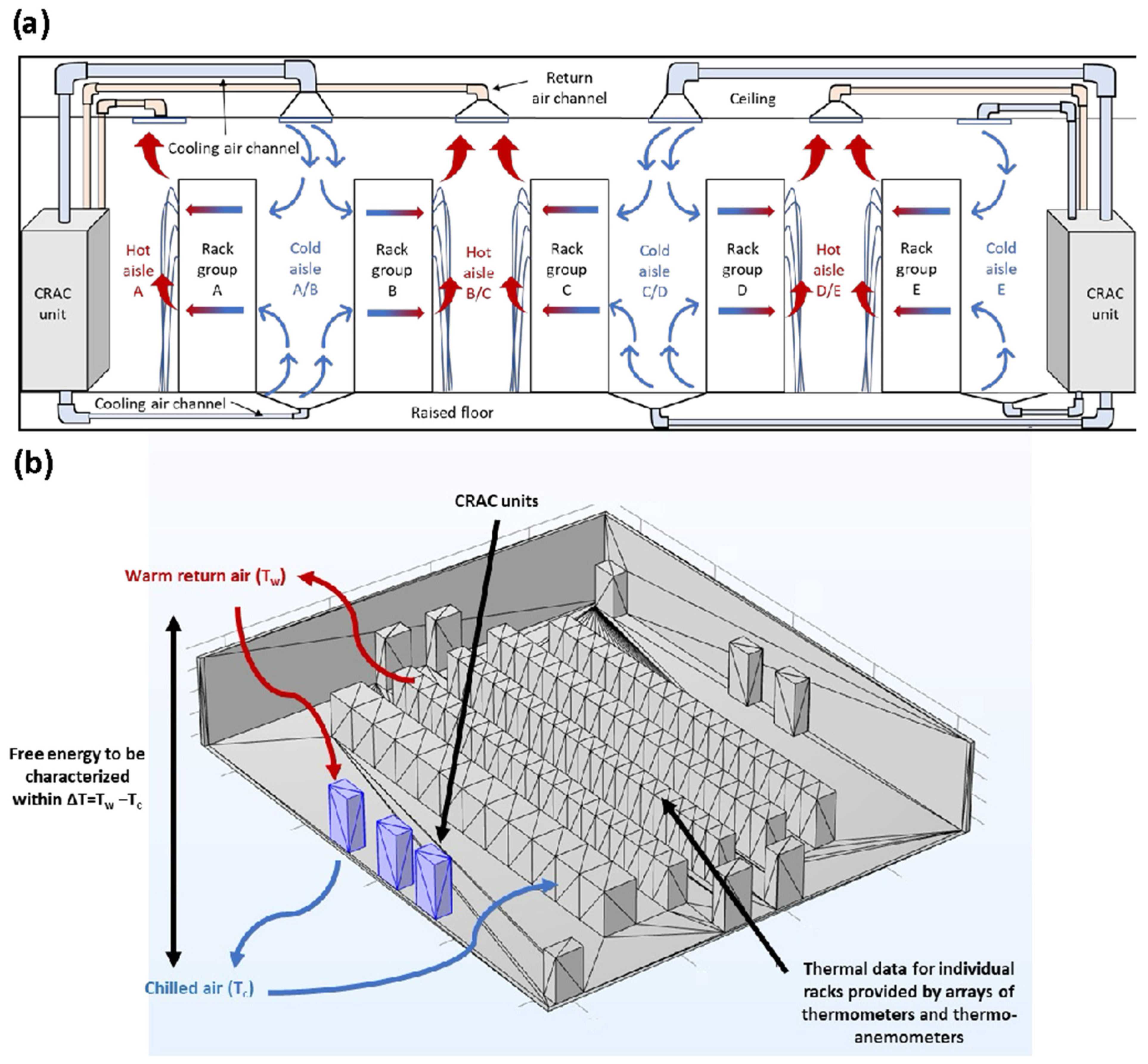
2.1. Server Room Selected for Simulation

In this study, the High-Performance Computing (HPC) server room of the Center for Advanced Research Computing (CARC) at the University of Southern California (USC) (Los Angeles, CA, USA) was used to represent a typical academic data center. The plan area of the server room is 288 m², with dimensions of 18, 16, and 4 m in length, width, and height. The room contains 2500 computer servers and several storage systems as well as high-speed network equipment in a five-row (A to E) configuration. The server room is cooled by nine CRAC units (seven in operation and two idle) that operate with air-based ventilation systems. Further details of the server room are provided in Appendix A

Table A1. Rack group and CRAC information.

Rack Group	Servers per Rack Group	CRAC Number	Operating Status
A	268	CRAC-1	ON
		CRAC-2	ON
B	592	CRAC-3	OFF
		CRAC-4	ON
C	588	CRAC-5	ON
		CRAC-6	ON
D	436	CRAC-7	OFF
		CRAC-8	ON
E	594	CRAC-9	ON

. Unless otherwise stated, “server room” in this paper refers to the HPC server room at USC.

2.2. Air-Cooling System in the Server Room

Figure 1a is a plan view of the server room showing the air-cooling system. The CRAC units cool air to 18 °C and emit the chilled air into the cold aisles of the server room via ceiling and ground vents. The server room has 72 ceiling cold vents (24 in each cold aisle) and 72 floor cold vents (24 in each cold aisle); each vent has length and width dimensions of 0.25 m. The servers in the rack groups draw the chilled air into their central processing units and graphic processing units, and, at the same time, emit hot exhaust that first mixes with the air in the hot aisle and is then drawn to the CRAC units via ceiling hot vents. The server room has 15 ceiling hot vents (5 in each hot aisle) with length and width dimensions of 0.58 m. The server room air-cooling system keeps the whole server room temperature relatively constant at approximately 21 °C. The cooling process is closed-loop; the CRAC units do not ventilate external air into the computer room, and thus, the airflow rate of warm return air entering the CRAC units and the airflow rate of chilled air emitted from the CRAC units are equal.

The energy required by the CRAC units is based on the temperature difference (ΔT) shown in Figure 1b. ΔT is the temperature difference between the inlet (i.e., return air shown by the red line) and outlet (i.e., chilled air shown by the blue line). The temperature difference describes the quality of the potential free energy that is emitted as waste heat. The quantity of the waste heat can be estimated based on the heat from the warm return air. If that waste heat is then transferred from the data center via a heat sink or heat exchange device, the waste heat can be reused. However, even if the heat is just emitted to the ambient environment, the cooling load on the CRAC units becomes reduced because taking the waste heat out of the server room (before it enters the CRAC units) decreases the return hot air temperature.

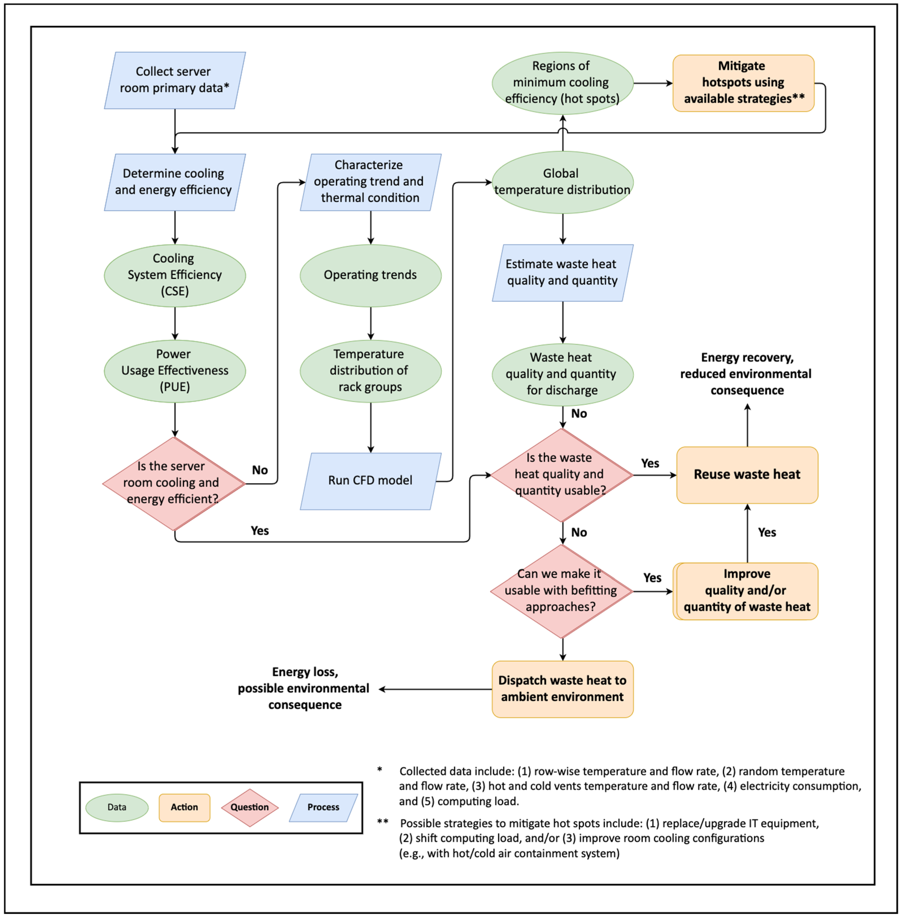
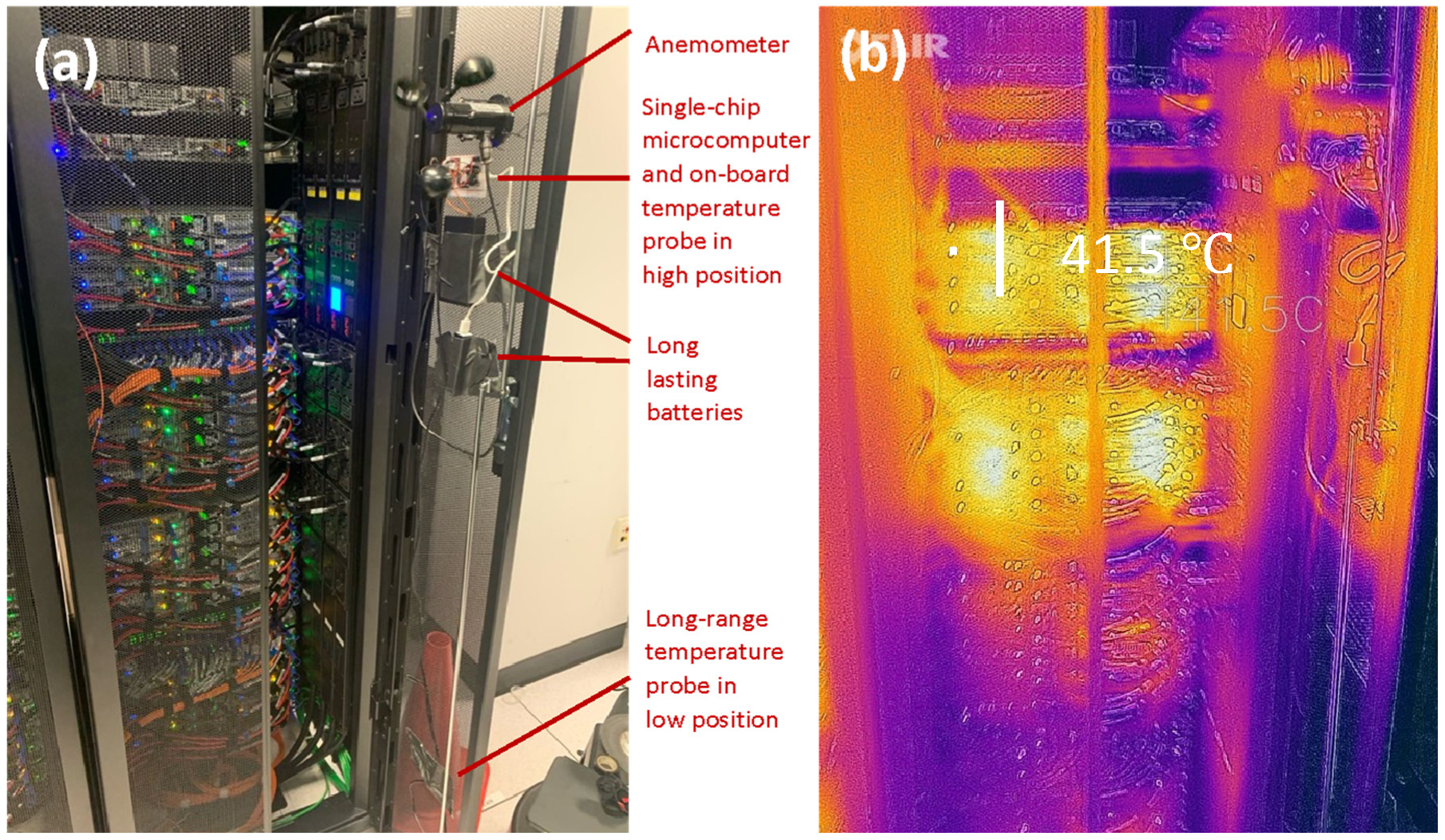
2.3. Analysis Framework and Collection of Primary Data

The analysis framework developed for typical academic data centers is shown in Figure 2 and detailed in the subsequent sections.

Because this server room was built in 2010 and does not utilize CRMS technology, primary data collection is the first step in the analysis framework. The primary data collected for the analysis include (a) row-wise temperature (T_ri in °C) and flow rate (q_ri in m³/s); (b) random temperature (T_xi in °C) and flow rate (q_xi in m³/s), where i represents one of the A to E rack groups in the server room; (c) hot and cold vent temperature (T_vi in °C) and flow rate (q_vi in m³/s); (d) electricity consumption over data collection time, t (Q_t in kWh); and (e) computing load (%; indicating mean CPU occupation as % of total capacity).

Row-wise thermal data were collected every ten minutes over one month using an array of 15 thermometers and 10 fabricated thermo-anemometers that were placed in the rack groups of the server room. The automated thermo-anemometers were each fabricated with a single-chip microcomputer (Raspberry Pi 4.0, Cambridge, UK), two temperature probes (Raspberry Pi Foundation, Cambridge, UK), one anemometer, and two long-lasting batteries (PKCell, Shenzhen, China). The thermometers and thermo-anemometers were coded with Python 3.0 to transmit and store the thermal data. The devices were installed following the “4-Points Rules” [41], which say that thermal data should be monitored at both low and high rack positions on both cold and hot aisles. Placement of the thermometers and anemometers in one of the hot-aisle racks is shown in Figure 3a. A thermogram of the rack (Figure 3b) taken using FLIR ONE Pro by Teledyne FLIR (Wilsonville, OR, UAS) shows the temperature distribution of the rack.

Random and hot- and cold-vent thermal data were measured intermittently over one month using hand-held, self-powered, thermo-anemometers (Digi-Sense Hot-Wire Thermo-anemometer UX-20250-16, Vernon Hills, USA). The accuracy of temperature measurement by the thermometers and thermo-anemometers is reported as 0.1 °C by the manufacturers. The accuracy of air velocity is reported as 0.01 m/s by the manufacturer. Systematic errors of ±1.5 °C for the air temperature and ±0.04 m/s for the air velocity (calibrated with nominal airflow velocity at 4.00 m/s) provide an indication of uncertainty in the measured data. The instruments were calibrated prior to use by the manufacturers at 23 °C under 54% RH and were tested in the data center for two weeks prior to data collection. The hand-held thermo-anemometers were used to collect thermal data at random locations within the hot aisle of each rack group (Appendix A

Table A2. Average temperatures and airflow rates at random locations in the hot aisles of the server room.

	Hot Aisle Temperature (°C)	Airflow Rate (m3/s)
Location 1 (in rack group A)	22.6	7.61
Location 2 (in rack group B)	31.0	16.4
Location 3 (in rack group C)	30.0	6.54
Location 4 (in rack group D)	45.4	3.66
Location 5 (in rack group E)	31.4	11.2
Average	32.1	9.07

). Average values of temperature and flow rate for the hot exhaust leaving through ceiling vents and chilled air entering through cold vents on the floor and ceiling are given in Appendix A

Table A3. Average temperatures and flow rates entering the hot vents and exiting the cold vents in the server room.

	Temperature (°C)	Airflow Rate (m3/s)
Hot vents ceiling	24.1	0.93
Cold vents floor	13.0	0.91
Cold vents ceiling	15.0	0.74

.

Electricity consumption for the server room was obtained from the facility’s monthly electricity bill. The average monthly electricity consumption for the server room is 354,050 kWh/month with an average electricity consumption of 177,025 kWh/month for the CRAC units specifically.

The computing load was obtained from the server room’s operating log that is documented on Grafana (version 7.4.3, Grafana Labs, New York, NY, USA). Representative durations (including one day, one week, and one month) were selected to represent peak scenarios (i.e., weekdays and mid-semester) and off-peak scenarios (i.e., weekends and off-semester). The data were used to identify operating trends for the data center.

2.4. Calculation of Cooling and Energy Efficiency Indices

The first question in the framework (Figure 1) (“Is the server room cooling and energy efficient?”) can be answered by calculating CSE and PUE using electricity consumption and global and row-wise thermal data.

CSE is given by the following [6]:

$$\mathrm{CSE}=\frac{Average Cooling System Power}{Average Cooling Load}$$

(1)

where average cooling system power is considered as the CRAC cooling power (kW), and average cooling load (ton of chilled air) is the cooling required to maintain a chilled-air temperature of 18 °C.

PUE is given by the following [6]:

$$\mathrm{PUE}=\frac{Total Facility Power}{ICT Equipment Power}$$

(2)

where ICT equipment power is the power required by server, storage, and network equipment, and total facility power (i.e., the power required to run the server room) comprises both ICT equipment power and auxiliary equipment power (e.g., lighting and HVAC). If CSE and PUE are better than or equal to the current industrial benchmarks (0.8 KW/ton for CSE and 1.6 for PUE) [15,42], the system is considered to be cooling- and energy-efficient and a waste heat analysis is performed (discussed later). If the system is considered to not be cooling and energy efficient, then the next step is to analyze operating trends and thermal conditions.

2.5. Characterization of Operating Trends and Thermal Conditions

Mean CPU occupation was used to characterize the server room operating trends for the daily, weekly, and monthly scenarios. For each scenario, peak and off-peak cases are categorized according to the following: (a) mid-semester (weekday), (b) mid-semester (weekend), (c) off-semester (weekday), and (d) off-semester (weekend). Row-wise temperature data collected from the hot and cold aisles for each rack group over a 30-day period was used to characterize the server room thermal conditions.

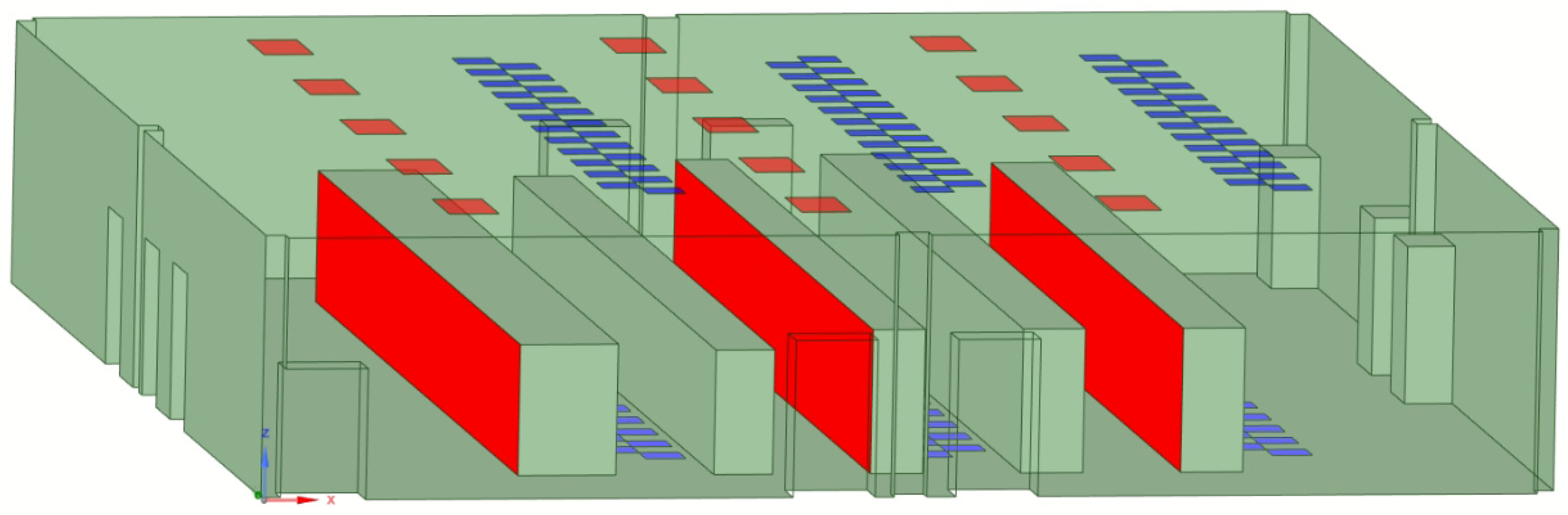
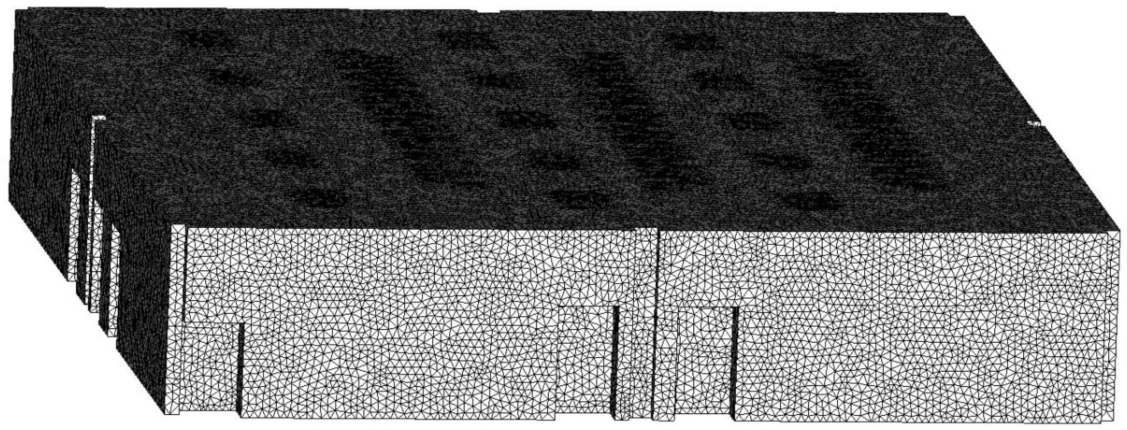
2.6. Development of CFD Model

A CFD model to simulate server room airflow and temperature was developed using ANSYS Workbench (Canonsburg, PA, USA); the room geometry was created, a computational mesh was generated, and CFD equations were solved. Figure 4 shows the HPC room geometry created using the SpaceClaim tool. The average temperature and velocity for the cold air coming from the ceiling vents were initially set at 18.0 °C and 0.35 m/s. The average temperature and air velocity for the cold air coming from the floor vents were initially set at 18.0 °C and 0.42 m/s.

The CFD computational surface mesh (Figure 5) was generated using triangular elements and the volume mesh was generated from the surface mesh with tetrahedral cells. Sizing limitations were applied to different regions of the domain to increase accuracy in a reasonable computational time. Limiting the mesh size to 25 cm in the whole domain and to 8 cm in the vicinity of the hot rack faces, hot vents, and cold vents resulted in 2,572,433 cells.

The CFD equations were solved using the realizable k-ε model, a one-phase model in Fluent with air (1.225 kg/m³ density) as its only material. This model was chosen because it allows turbulence when describing air mass- and heat-transfer properties. The near-wall treatment in the k-ε model was considered a non-equilibrium wall function. The global temperature distribution was then determined by the heat map generated in Fluent.

2.7. Estimation of Server Room Waste Heat Quality and Quantity

The annual collectable potential energy due to changes in the internal energy of air with a temperature difference in the CRAC units in the server room (ΔU in MWh) was calculated using the following:

$$\Delta U=\Delta W\times t$$

(3)

where t is time (h) and $\Delta W$ is the heat power (kW) that can be calculated from the potential waste heat collected from the server room and is given by the following:

$$\Delta W=\dot{m}\times C_{air,T_r}\times \Delta T$$

(4)

where $\dot{m}$ is the mass flow rate (kg/s) of the hot exhaust that enters each ceiling hot vent (see below). $C_{air,T_r}$ is the specific heat capacity (kJ·kg⁻¹·K⁻¹) for air at the temperature of the returned hot exhaust, which is equal to 1.0061 kJ·kg⁻¹·K⁻¹ (at 1 atm pressure). $\Delta T$ (in °C) is the temperature difference in the CRAC units:

$$\Delta T=T_w-T_c$$

(5)

where T_w is warm return air temperature from the ceiling hot vents and T_c is chilled air temperature blowing into the server room from the CRAC units.

$\dot{m}$ from Equation (4) is given by the following:

$$\dot{m}=\dot{q}\times \rho$$

(6)

where $\rho$ is the air density (kg/m³) determined based on the average temperature of the returned hot exhaust and $\dot{q}$ (m³·s⁻¹) is the airflow rate for the returned air entering the 15 hot vents and is given by the following:

$$\dot{q}=v_{avg}\times A\times 15$$

(7)

where $v_{avg}$ is the average hot vent airflow velocity (m/s) and A is the area of each hot vent (0.34 m²).

3. Results and Discussion

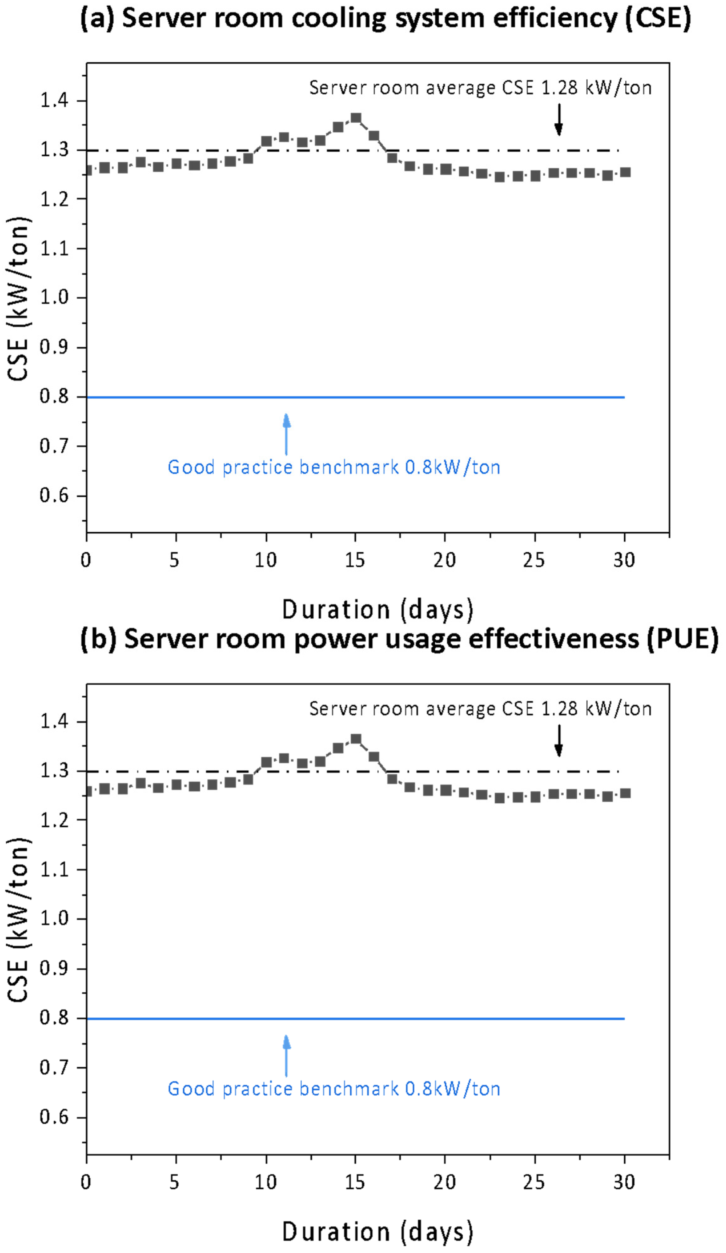
3.1. Server Room CSE and PUE

The data in Figure 6 show CSE and PUE indices calculated for the server room over one month. In Figure 6a, the daily CSE values range from 1.25 to 1.37 KW/ton; the 30-day average is 1.28 kW/ton. This average value is higher than the good practice benchmark of 0.8 kW/ton [16,17]. In Figure 6b, the daily PUE value ranges from 1.7 to 5.2; the 30-day average is 2.5. This average value is higher than the US average value of 1.6 [8].

The average CSE and PUE values in this study indicate cooling and energy inefficiencies that are not unexpected in academic data centers. Cooling system inefficiencies may be due to chilled air bypassing and short-circuiting in the open-aisle configuration (Figure 1a). Cooling system inefficiencies may also result from slow responses of the cooling system to changes in computing load, which are discussed in the next section.

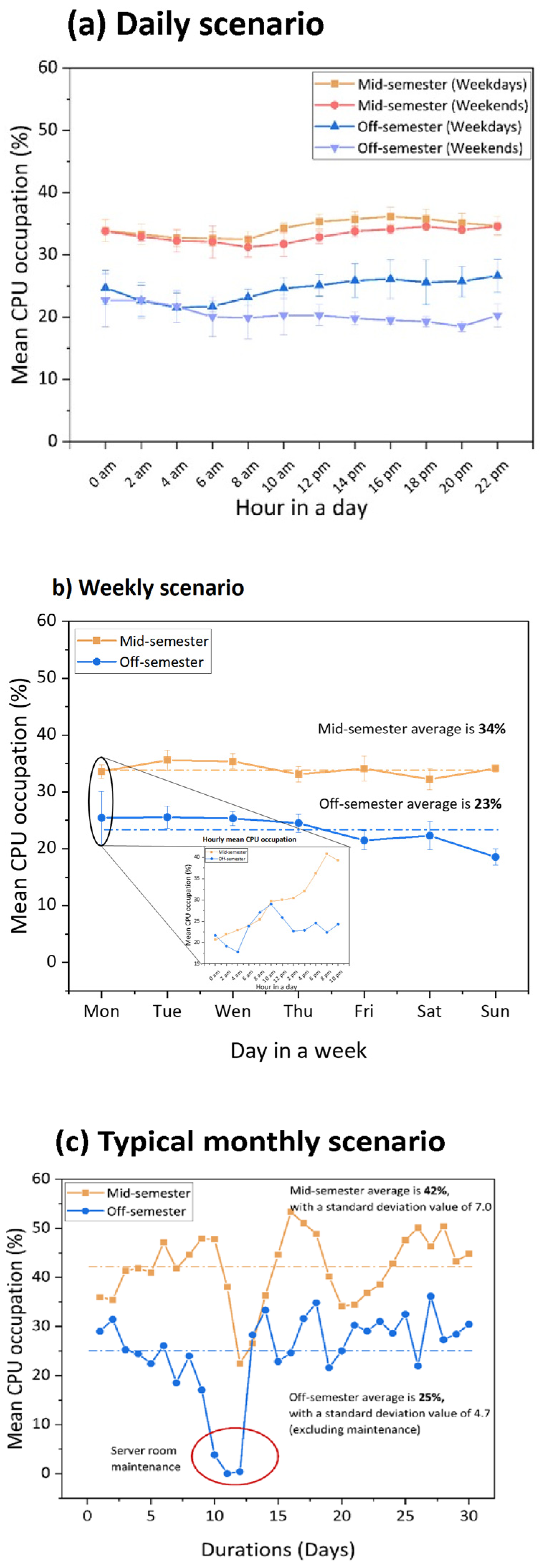
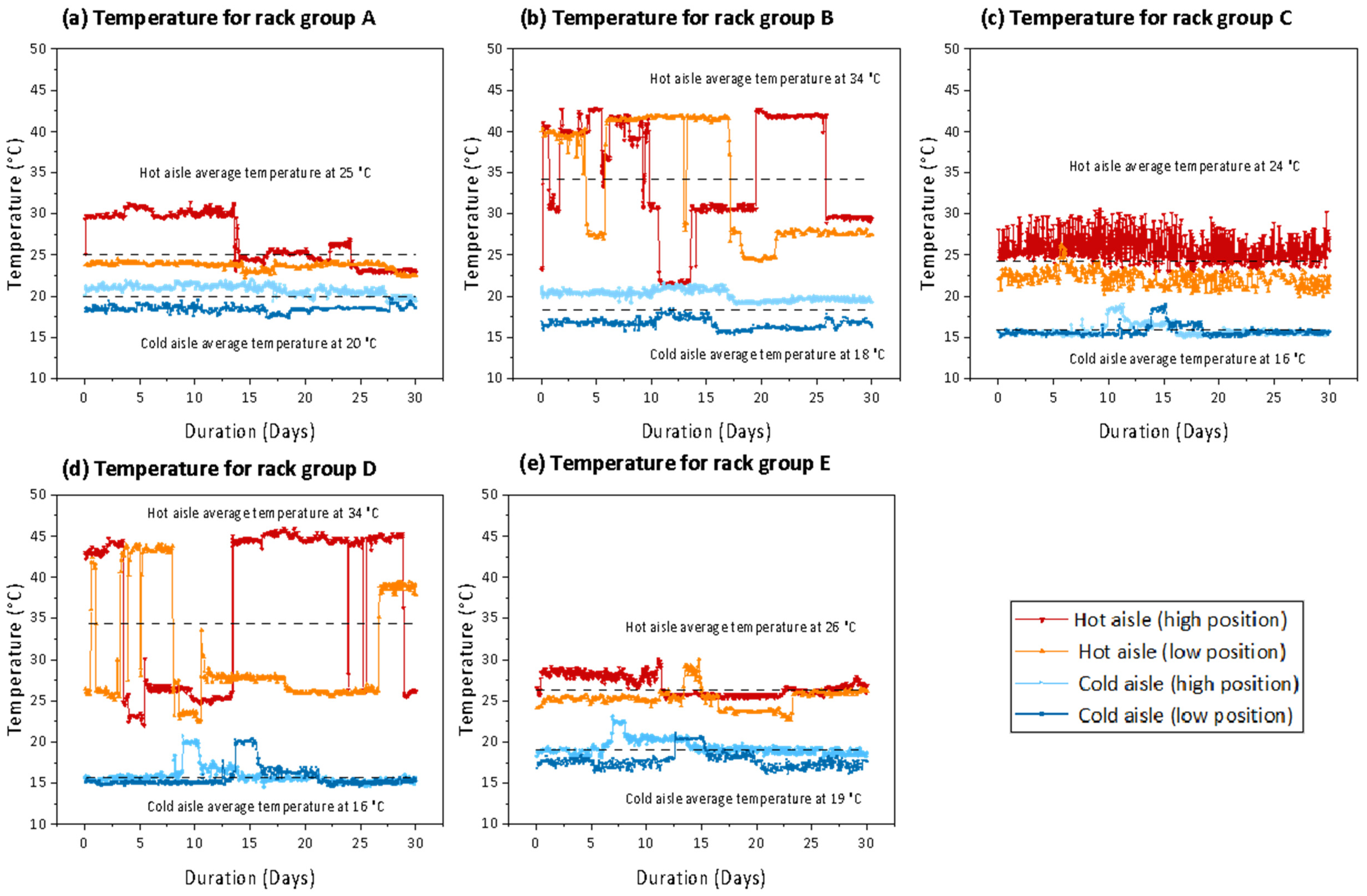
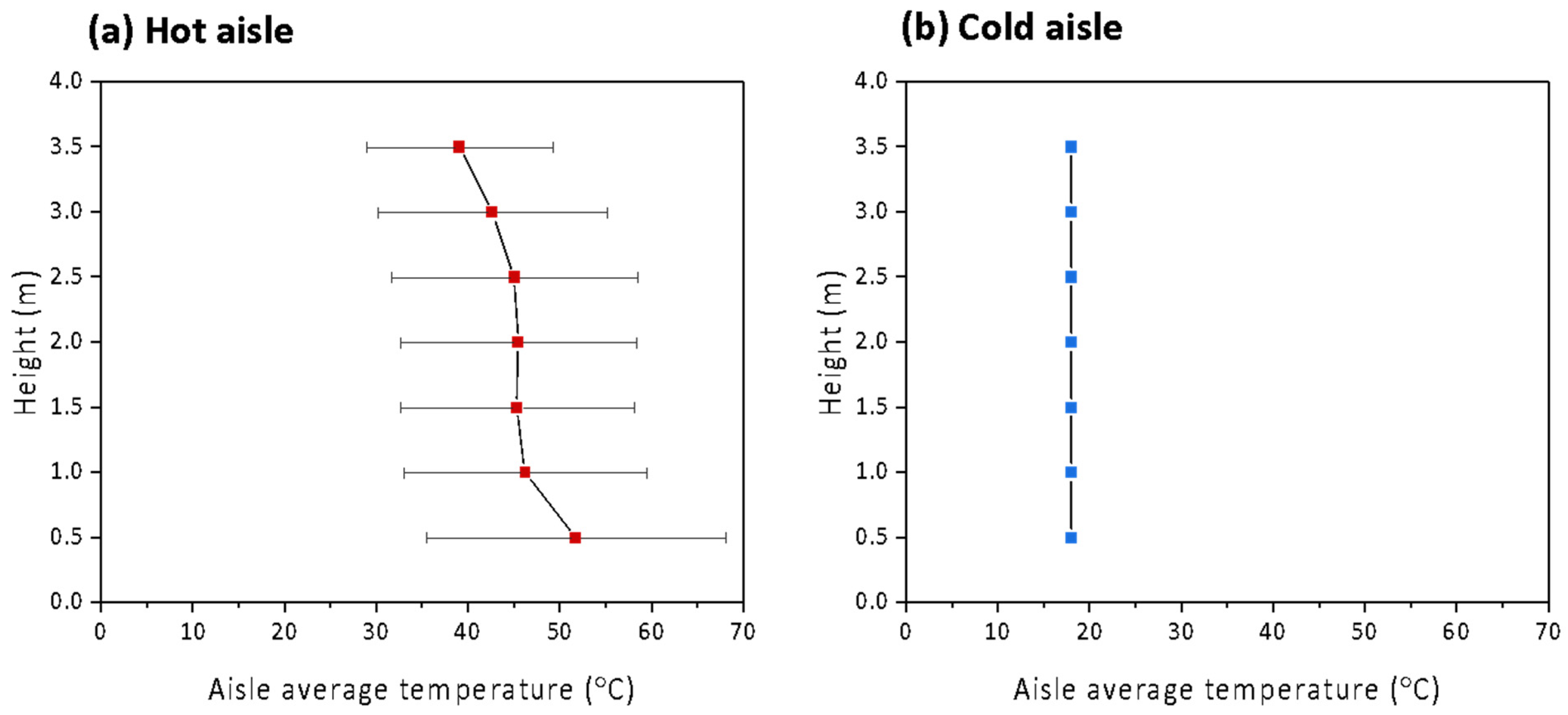
3.2. Server Room Operating Trends and Temperature Distribution

Mean CPU occupation data (Figure 7) shows the variability of the workload on the servers. Looking at the daily scenario (Figure 7a), the mean CPU occupation starts increasing after 8 am and reaches the highest value in the afternoon (except for weekends in the off-semester). In all cases, CPU occupation ranges from 19 to 37%. In the weekly scenario (Figure 7b), the mean CPU occupation ranges from 17 to 39% with the average off-semester mean CPU occupation (23%) less than the mid-semester mean CPU occupation (34%). The inset graph in Figure 7b shows the raw hourly data. These data have high variability that is not observed in Figure 7a where the hourly data has been averaged. A typical monthly scenario is shown in Figure 7c. Mean CPU occupation ranges from 17 to 53% (excluding the period of server-room maintenance) and, as expected, the off-semester mean CPU occupation is generally less than the mid-semester mean CPU occupation. Server room CPU occupation trends can be concluded as (a) the average server room mean CPU occupation is less than 50% for the time period considered; (b) CPU occupation is almost always greater in mid-semester than off-semester and is generally less on weekends than weekdays; and (c) the daily variability of mean CPU occupation can range from 20 to 50% in mid-semester. Because this large variability cannot be mitigated by more advanced cooling systems with faster response time, the result is decreased cooling system efficiency.

The data in Figure 8 show the temperature data for each rack group collected over one month. The average hot-aisle temperatures have a wider range (24 to 34 °C) than the average cold-aisle temperatures (16 to 20 °C). The hot-aisle variability for rack groups B and D is greater than it is for rack groups A, C, and E. The servers in rack groups B and D have mixed ownership, with some of the servers belonging to individual research groups. The use of the servers depends on each group’s research agenda, which results in surges between full operation and cool-down periods depending on project due dates and publication schedules. Also, the hot aisles (especially for rack groups B and D) have greater vertical temperature variability in that sometimes the high position is warmer than the low position, and sometimes the high position is cooler. The greater stability and fewer fluctuations in cold aisle temperature are likely because the cold aisle has vents in both the ceiling and floor, whereas the hot aisle only has vents in the ceiling. Other likely reasons for uneven hot-aisle temperature distributions are the nonuniform cooling loads and unevenly distributed rack server density that is common in academic data centers.

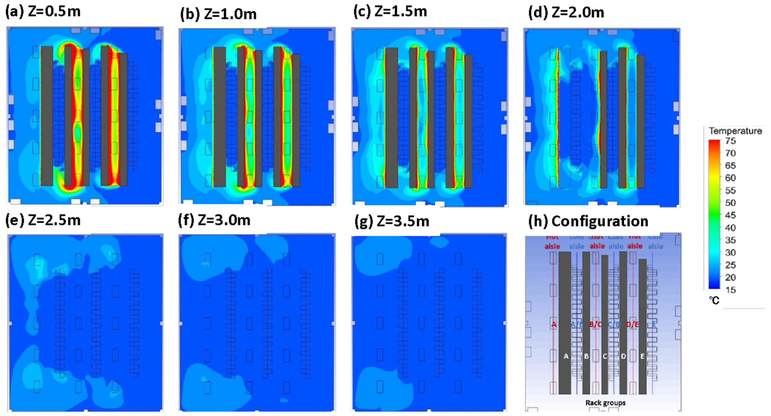
3.3. Server Room Waste Heat Estimation and Reuse Analysis from CFD Model Results

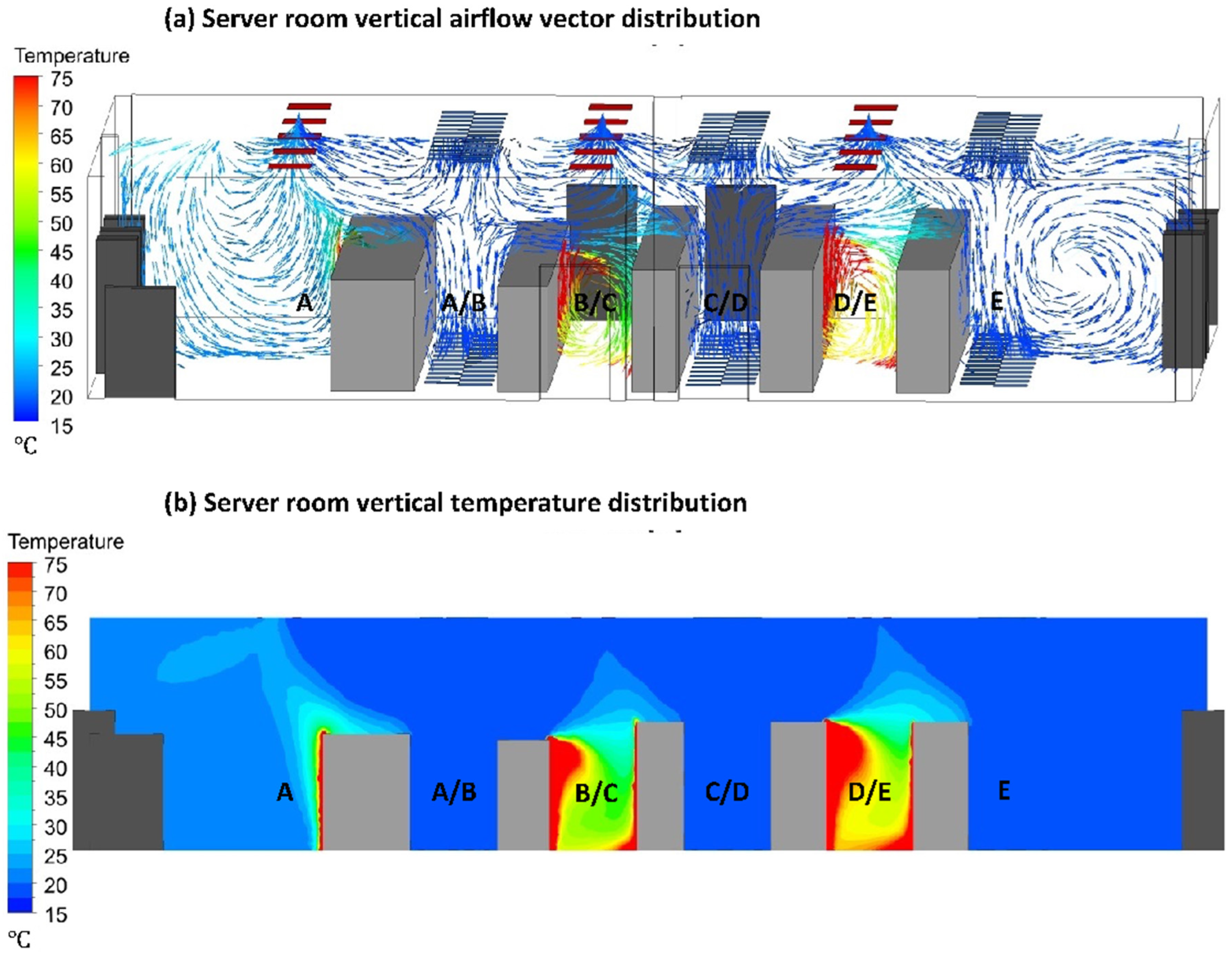
3.3.1. Current Server Room Configuration with Open Aisles

CFD simulation results are shown as a temperature contour plot in Figure 9. Figure 9a–g show temperature distribution at heights of 0.5 to 3.5 m in 0.5 m increments; Figure 9h provides a reminder of the server room aisle and rack group configuration. In Figure 9e–g, only outlines of the five rack groups are shown because the rack height is shorter than 2.5 m. Looking at Figure 9a–d, hot aisles B/C and D/E are hotter than hot aisle A. Looking at Figure 9a–g, hot exhaust temperatures decrease with distance from the floor (i.e., temperatures decrease as the hot exhaust rises). Clearly, there are some regions in the server room where temperatures are significantly higher than in adjacent regions; these hot spots are indicated by red coloring. Hot spots can be mitigated by three strategies: replacing or upgrading the ICT equipment (e.g., [43]), shifting the computing load (e.g., [44]), or improving the room cooling configuration (e.g., [45]). In this study, a hot-air containment system (HAC) system is simulated to mitigate hot spots (discussed in Section 3.3.2).

Figure 9a–d also show that the hot air from the hot aisles diffuses into open space as it rises. And when it enters the space above the rack groups (Figure 9e–g), chilled air has chilled it prior to it entering the return air channel. Some chilled air bypasses the server inlets where it should be cooling the servers; this is shown in more detail in Figure 10.

The airflow vectors in Figure 10a show that the hot exhaust emitted by the servers into aisles B/C and D/E is trapped by chilled air coming from the cold aisles. This chilled air is bypassing the server inlets where it should be cooling the servers. This short-circuiting leads to less cooling of the servers and hotter exhaust entering the hot aisles. Figure 10b shows the resulting vertical temperature distribution in a sectional slice of the server room, which clearly indicates the vertical distribution of the hot spots. The vertical average hot ailse air temperature distribution in Figure 11a shows that the average hot exhuast temperature in the hot aisles decreases from approximately 47 °C on the floor to approximately 20 °C on the ceiling; and the temperatures of the chilled air in the cold aisles in Figure 11b is relatively constant at 18 °C.

According to the CFD simulation results (

Table 1. Average air temperature for hot and cold aisles in the server room with open aisles.

Height (m)	Aisle Temperature (°C)
	Aisle A	Aisle A/B	Aisle B/C	Aisle C/D	Aisle D/E	Aisle E
0.5	25.1	18.3	51.4	18.3	64.5	18.0
1.0	25.8	18.6	49.0	18.5	56.4	18.0
1.5	26.7	18.8	41.8	18.6	47.2	18.0
2.0	27.9	18.8	29.1	18.6	34.1	18.0
2.5	27.5	18.5	22.4	18.4	23.4	18.0
3.0	24.4	18.2	19.9	18.1	20.1	18.0
3.5	21.5	18.1	19.0	18.0	19.0	18.0

), cold-aisle temperatures in aisle C/D increase from 18.0 (the initial chilled air temperature entering from the vents) to 18.5 °C. Although the bypass effect causes the air entering the CRAC units from the hot aisles to be cooler than it would otherwise be, the CRAC units operate based on the temperature of the cold aisles. Thus, more energy is required to maintain the target cooling temperature (18.0 °C) and satisfy server cooling needs. The increased energy requirements due to the bypass effect contributes to the higher PUE and CSE values for the data center. Furthermore, data center managers are often more concerned with cold-aisle temperatures, which are often seen as an indicator of overall cooling efficiency [46].

The current server room configuration with open aisles has an average return air temperature of 23 °C (with a dry air density of 1.19 kg/m³ at 1 atm). If the reuse of the waste heat is being considered, 23 °C is low quality compared to the district heating target of 40 °C reported in the literature [16,30,31]. The theoretical ΔT that can be obtained is only approximately 5 °C. Using Equations (3)–(7) and a warm air velocity of 1.41 m/s, a heat power ($\Delta W$) of 43.1 kW of waste heat is emitted via a cooling tower on the data center roof. For one year of continuous operation, this is calculated as 377 MWh of emitted waste heat.

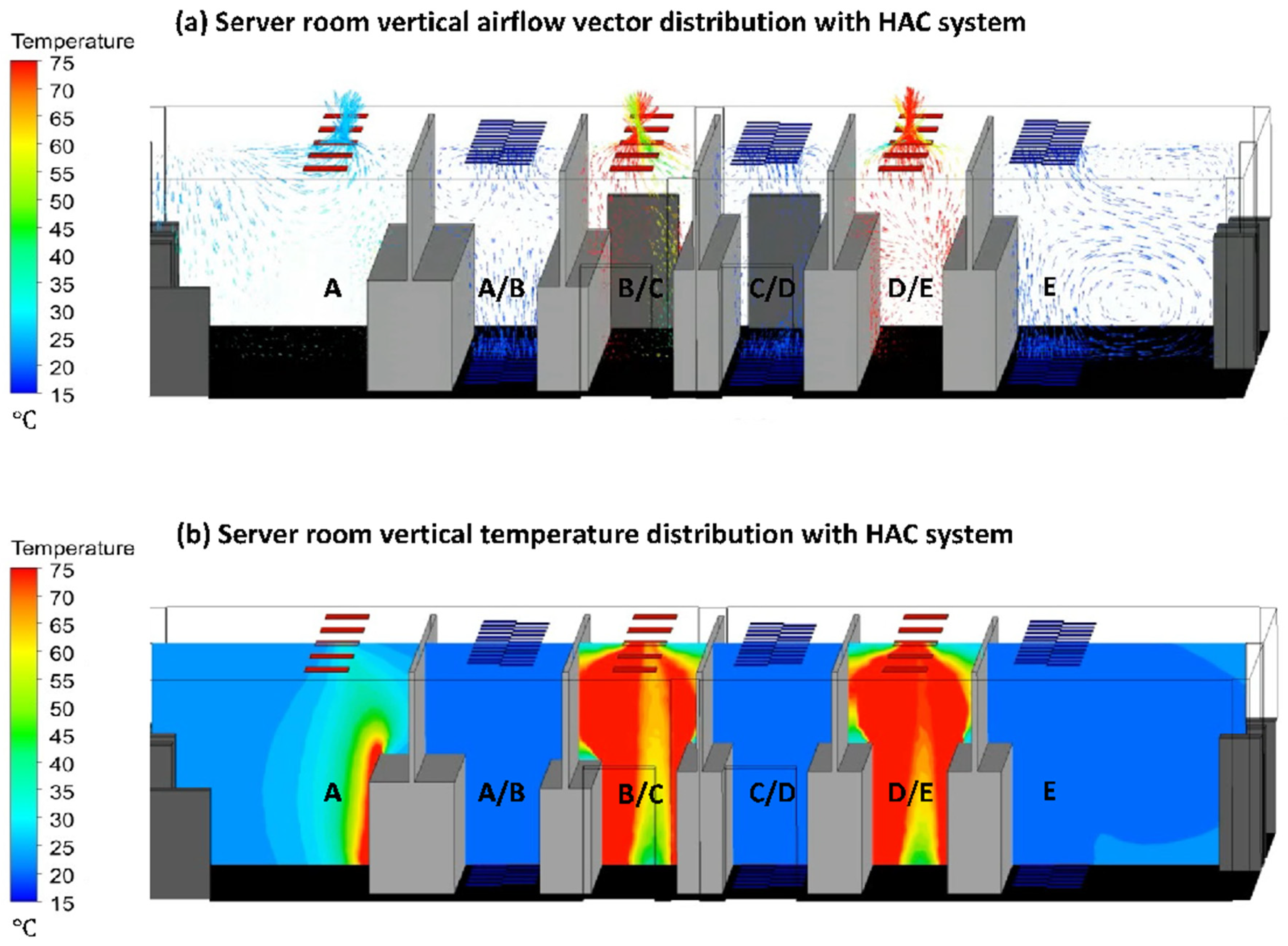
3.3.2. Example of Improved Server Room Configuration with HAC System

CFD simulation results for the improved server room with an HAC system are shown in Figure 12. As can be seen in Figure 12a, the HAC system confines the hot exhaust and prohibits it from mixing with the chilled air after leaving the hot aisles. Because the hot exhaust in aisles B/C and D/E is contained, the aisle temperatures are much higher than they are in Figure 10a. Figure 12b shows that the HAC system prevents chilled air from bypassing the server inlets; instead, chilled air is available to cool the servers.

According to the CFD simulation results (

Table 2. Average air temperature for hot and cold aisles in the server room with the hot air containment system.

Height (m)	Aisle Temperature (°C)
	Aisle A	Aisle A/B	Aisle B/C	Aisle C/D	Aisle D/E	Aisle E
0.5	31.1	18.0	53.1	18.0	70.9	18.0
1.0	28.1	18.0	50.8	18.0	59.7	18.0
1.5	27.3	18.0	53.0	18.0	55.7	18.0
2.0	27.2	18.0	55.7	18.0	53.4	18.0
2.5	26.2	18.0	56.4	18.0	52.6	18.0
3.0	25.2	18.0	53.7	18.0	49.0	18.0
3.5	24.7	18.0	47.5	18.0	44.9	18.0

) and the average hot/cold aisle temperatures shown in Figure 13, the improved server room configuration with an HAC system has an average return air temperature of 46 °C (with a dry air density of 1.11 kg/m³ at 1 atm), which is twice that of the open-aisle configuration. The improved return air temperature exceeds the district heating target of 40 °C reported in the literature [30,31,47]. The theoretical ΔT that can be obtained is approximately 28 °C with a warm air velocity of 1.44 m/s. A heat power ($\Delta W$) of 289 kW of waste heat is emitted via the cooling tower on the data center roof. The quality of this waste heat is much higher than in the open-aisle configuration and represents waste heat that may be worthwhile to reuse for auxiliary equipment, similar to the leading commercial data centers (e.g., Amazon, Google, and Microsoft). With an average return air temperature of 46 °C, for one year of continuous operation, this is calculated as 2004 MWh of waste heat. Compared to the open-aisle configuration, the configuration with the HAC system has returned air that is two times warmer and can produce five times more energy. Also, it can be seen that this annual waste heat quantity (2004 MWh) is just below the range of those from the literature (3156–11,045 MWh in [11,37,38,39,40]).

4. Conclusions and Implications

In this study, real-time onsite waste heat data were collected and an analysis framework was developed to characterize the quality and quantity of waste heat from a typical academic data center. CFD simulations found that waste heat quality for the server room was low (23 °C) and less than the district heating target of 40 °C reported in the literature. However, by implementing a basic hot air management approach (an HAC system), cooling efficiency increased and the temperature doubled (to 46 °C). Five times more energy is produced in the HAC configuration than in the open-aisle configuration (2004 vs. 377 MWh annually). Our study emphasizes that containing waste heat is the first step in making it available for reuse, and that containment can significantly increase its quality. It should be noted that liquid cooling systems inherently contain waste heat and, given the renewed interest in these systems [48], opportunities for waste heat reuse are only expected to grow. Further, opportunities to upgrade the waste heat to a higher quality using heat concentration technology (e.g., a heat pump system) will be critical in analyzing the mechanics and cost of reusing waste heat. And in general, the robust growth in the data center cooling market (from USD 12.7 billion today to 29.6 billion by 2028) bodes well for further improvements to system efficiency, especially since the research and academic sector is projected to have the highest growth rate [49].

In addition to the value of recovering waste heat as a resource, there may be value in not releasing the waste heat to the ambient environment. This is particularly true if the data center is located in an urban setting where surface heating contributes to the urban heat island effect or disturbance of the ambient environment is a concern in cold areas [9]. For urban environments, use of a waste heat data set in a broader analysis of the environmental impact of anthropogenic heat emitted by industrial and residential buildings would be beneficial. And specifically for academic data centers, as universities look to be more sustainable and operate more efficiently [10], opportunities to operate with minimal unintended consequences and a lifecycle mindset may be valued.

References

1. Dayarathna, M.; Wen, Y.; Fan, R. Data center energy consumption modeling: A survey. IEEE Commun. Surv. Tutor. 2015, 18, 732–794. [Google Scholar] [CrossRef]
2. Masanet, E.; Shehabi, A.; Lei, N.; Smith, S.; Koomey, J. Recalibrating global data center energy-use estimates. Science 2020, 367, 984–986. [Google Scholar] [CrossRef] [PubMed]
3. Achiam, J.; Adler, S.; Agarwal, S.; Ahmad, L.; Akkaya, I.; Aleman, F.L.; Almeida, D.; Altenschmidt, J.; Altman, S.; Anadkat, S.; et al. GPT-4 Technical Report. arXiv 2023, arXiv:2303.08774. [Google Scholar]
4. Poess, M.; Nambiar, R.O. Energy cost, the key challenge of today’s data centers: A power consumption analysis of TPC-C results. Proc. VLDB Endow. 2008, 1, 1229–1240. [Google Scholar] [CrossRef]
5. Kamiya, G. Data Centres and Data Transmission Networks. Available online: https://www.iea.org/reports/data-centres-and-data-transmission-networks (accessed on 24 February 2024).
6. Capozzoli, A.; Chinnici, M.; Perino, M.; Serale, G. Review on performance metrics for energy efficiency in data center: The role of thermal management. In Proceedings of the International Workshop on Energy Efficient Data Centers, Cambridge, UK, 10 June 2014; Springer: Berlin/Heidelberg, Germany, 2014; pp. 135–151. [Google Scholar]
7. Long, S.; Li, Y.; Huang, J.; Li, Z.; Li, Y. A review of energy efficiency evaluation technologies in cloud data centers. Energy Build. 2022, 260, 111848. [Google Scholar] [CrossRef]
8. Lee, Y.-T.; Wen, C.-Y.; Shih, Y.-C.; Li, Z.; Yang, A.-S. Numerical and experimental investigations on thermal management for data center with cold aisle containment configuration. Appl. Energy 2022, 307, 118213. [Google Scholar] [CrossRef]
9. Baniata, H.; Mahmood, S.; Kertesz, A. Assessing anthropogenic heat flux of public cloud data centers: Current and future trends. PeerJ Comput. Sci. 2021, 7, e478. [Google Scholar] [CrossRef] [PubMed]
10. Choo, K.; Galante, R.M.; Ohadi, M.M. Energy consumption analysis of a medium-size primary data center in an academic campus. Energy Build. 2014, 76, 414–421. [Google Scholar] [CrossRef]
11. Dvorak, V.; Zavrel, V.; Torrens Galdiz, J.; Hensen, J.L. Simulation-based assessment of data center waste heat utilization using aquifer thermal energy storage of a university campus. In Building Simulation; Springer: Berlin/Heidelberg, Germany, 2020; Volume 13, pp. 823–836. [Google Scholar]
12. Ali, E. Energy efficient configuration of membrane distillation units for brackish water desalination using exergy analysis. Chem. Eng. Res. Des. 2017, 125, 245–256. [Google Scholar] [CrossRef]
13. Cho, J.; Lim, T.; Kim, B.S. Viability of datacenter cooling systems for energy efficiency in temperate or subtropical regions: Case study. Energy Build. 2012, 55, 189–197. [Google Scholar] [CrossRef]
14. Karimi, L.; Yacuel, L.; Degraft-Johnson, J.; Ashby, J.; Green, M.; Renner, M.; Bergman, A.; Norwood, R.; Hickenbottom, K.L. Water-energy tradeoffs in data centers: A case study in hot-arid climates. Resour. Conserv. Recycl. 2022, 181, 106194. [Google Scholar] [CrossRef]
15. Greenberg, S.; Mills, E.; Tschudi, B.; Rumsey, P.; Myatt, B. Best practices for data centers: Lessons learned from benchmarking 22 data centers. In Proceedings of the ACEEE Summer Study on Energy Efficiency in Buildings, Asilomar, CA, USA, 13–18 August 2006; Volume 3, pp. 76–87. [Google Scholar]
16. Wang, L.; Khan, S.U. Review of performance metrics for green data centers: A taxonomy study. J. Supercomput. 2013, 63, 639–656. [Google Scholar] [CrossRef]
17. Mathew, P.; Ganguly, S.; Greenberg, S.; Sartor, D. Self-Benchmarking Guide for Data Centers: Metrics, Benchmarks, Actions; Lawrence Berkeley National Lab. (LBNL): Berkeley, CA, USA, 2009. [Google Scholar]
18. Pärssinen, M.; Wahlroos, M.; Manner, J.; Syri, S. Waste heat from data centers: An investment analysis. Sustain. Cities Soc. 2019, 44, 428–444. [Google Scholar] [CrossRef]
19. Lu, T.; Lü, X.; Remes, M.; Viljanen, M. Investigation of air management and energy performance in a data center in Finland: Case study. Energy Build. 2011, 43, 3360–3372. [Google Scholar] [CrossRef]
20. Monroe, M. How to Reuse Waste Heat from Data Centers Intelligently; Data Center Knowledge: West Chester Township, OH, USA, 2016. [Google Scholar]
21. Wahlroos, M.; Pärssinen, M.; Rinne, S.; Syri, S.; Manner, J. Future views on waste heat utilization–Case of data centers in Northern Europe. Renew. Sustain. Energy Rev. 2018, 82, 1749–1764. [Google Scholar] [CrossRef]
22. Velkova, J. Thermopolitics of data: Cloud infrastructures and energy futures. Cult. Stud. 2021, 35, 663–683. [Google Scholar] [CrossRef]
23. Vela, J. Helsinki data centre to heat homes. The Guardian, 20 July 2010. Available online: https://www.theguardian.com/environment/2010/jul/20/helsinki-data-centre-heat-homes(accessed on 24 February 2024).
24. Fontecchio, M. Companies Reuse Data Center Waste Heat to Improve Energy Efficiency; TechTarget SearchDataCenter: Newton, MA, USA, 2008. [Google Scholar]
25. Miller, R. Data Center Used to Heat Swimming Pool; Data Center Knowledge: West Chester Township, OH, USA, 2008; Volume 2. [Google Scholar]
26. Oró, E.; Taddeo, P.; Salom, J. Waste heat recovery from urban air cooled data centres to increase energy efficiency of district heating networks. Sustain. Cities Soc. 2019, 45, 522–542. [Google Scholar] [CrossRef]
27. Nerell, J. Heat Recovery from Data Centres. Available online: https://eu-mayors.ec.europa.eu/sites/default/files/2023-10/2023_CoMo_CaseStudy_Stockholm_EN.pdf (accessed on 24 February 2024).
28. Westin Building Exchange. 2018. Available online: https://www.westinbldg.com/Content/PDF/WBX_Fact_Sheet.pdf (accessed on 24 February 2024).
29. Nieminen, T. Fortum and Microsoft’s Data Centre Project Advances Climate Targets. Available online: https://www.fortum.com/data-centres-helsinki-region (accessed on 24 February 2024).
30. Huang, P.; Copertaro, B.; Zhang, X.; Shen, J.; Löfgren, I.; Rönnelid, M.; Fahlen, J.; Andersson, D.; Svanfeldt, M. A review of data centers as prosumers in district energy systems: Renewable energy integration and waste heat reuse for district heating. Appl. Energy 2020, 258, 114109. [Google Scholar] [CrossRef]
31. Ebrahimi, K.; Jones, G.F.; Fleischer, A.S. A review of data center cooling technology, operating conditions and the corresponding low-grade waste heat recovery opportunities. Renew. Sustain. Energy Rev. 2014, 31, 622–638. [Google Scholar] [CrossRef]
32. Sandberg, M.; Risberg, M.; Ljung, A.-L.; Varagnolo, D.; Xiong, D.; Nilsson, M. A modelling methodology for assessing use of datacenter waste heat in greenhouses. In Proceedings of the Third International Conference on Environmental Science and Technology, ICOEST, Budapest, Hungary, 19–23 October 2017. [Google Scholar]
33. Mountain, G. Land-Based Lobster Farming Will Use Waste Heat from Data Center. Available online: https://greenmountain.no/data-center-heat-reuse/ (accessed on 24 February 2024).
34. White Data Center Inc. The Commencement of Japanese Eel Farming. Available online: https://corp.wdc.co.jp/en/news/2024/01/240/ (accessed on 24 February 2024).
35. Data Center Optimization Initiative (DCOI). Available online: https://viz.ogp-mgmt.fcs.gsa.gov/data-center-v2 (accessed on 24 February 2024).
36. Moss, S. Available online: https://www.datacenterdynamics.com/en/news/giant-us-federal-spending-bill-includes-data-center-energy-efficiency-measures/ (accessed on 24 February 2024).
37. Oltmanns, J.; Sauerwein, D.; Dammel, F.; Stephan, P.; Kuhn, C. Potential for waste heat utilization of hot-water-cooled data centers: A case study. Energy Sci. Eng. 2020, 8, 1793–1810. [Google Scholar] [CrossRef]
38. Hou, J.; Li, H.; Nord, N.; Huang, G. Model predictive control for a university heat prosumer with data centre waste heat and thermal energy storage. Energy 2023, 267, 126579. [Google Scholar] [CrossRef]
39. Montagud-Montalvá, C.; Navarro-Peris, E.; Gómez-Navarro, T.; Masip-Sanchis, X.; Prades-Gil, C. Recovery of waste heat from data centres for decarbonisation of university campuses in a Mediterranean climate. Energy Convers. Manag. 2023, 290, 117212. [Google Scholar] [CrossRef]
40. Li, H.; Hou, J.; Hong, T.; Ding, Y.; Nord, N. Energy, economic, and environmental analysis of integration of thermal energy storage into district heating systems using waste heat from data centres. Energy 2021, 219, 119582. [Google Scholar] [CrossRef]
41. ISO/IEC 30134-2:2016; Key Performance Indicators Part 2: Power Usage Effectiveness (PUE). International Organization for Standardization (ISO): Geneva, Switzerland, 2018.
42. Nadjahi, C.; Louahlia, H.; Lemasson, S. A review of thermal management and innovative cooling strategies for data center. Sustain. Comput. Inform. Syst. 2018, 19, 14–28. [Google Scholar] [CrossRef]
43. Amiri Delouei, A.; Sajjadi, H.; Ahmadi, G. Ultrasonic vibration technology to improve the thermal performance of CPU water-cooling systems: Experimental investigation. Water 2022, 14, 4000. [Google Scholar] [CrossRef]
44. Wang, J.; Deng, H.; Liu, Y.; Guo, Z.; Wang, Y. Coordinated optimal scheduling of integrated energy system for data center based on computing load shifting. Energy 2023, 267, 126585. [Google Scholar] [CrossRef]
45. Fulpagare, Y.; Bhargav, A. Advances in data center thermal management. Renew. Sustain. Energy Rev. 2015, 43, 981–996. [Google Scholar] [CrossRef]
46. Alissa, H.; Nemati, K.; Sammakia, B.; Ghose, K.; Seymour, M.; Schmidt, R. Innovative approaches of experimentally guided CFD modeling for data centers. In Proceedings of the 2015 31st Thermal Measurement, Modeling & Management Symposium (SEMI-THERM), San Jose, CA, USA, 15–19 March 2015; pp. 176–184. [Google Scholar]
47. Wahlroos, M.; Pärssinen, M.; Manner, J.; Syri, S. Utilizing data center waste heat in district heating–Impacts on energy efficiency and prospects for low-temperature district heating networks. Energy 2017, 140, 1228–1238. [Google Scholar] [CrossRef]
48. Li, P.; Yang, J.; Islam, M.A.; Ren, S. Making ai less “thirsty”: Uncovering and addressing the secret water footprint of ai models. arXiv 2023, arXiv:2304.03271. [Google Scholar]
49. Data Center Cooling Market by Solution (Air Conditioning, Chilling Unit, Cooling Tower, Economizer System, liquid Cooling System, Control System), Service, Type of Cooling, Data Center Type, Industry, & Geography—Global Forecast to 2030. 2024. Available online: https://www.marketsandmarkets.com/Market-Reports/data-center-cooling-solutions-market-1038.html (accessed on 8 March 2024).
Figure 1. (a) Section view of the server room. Air is circulated by computer room air-conditioning (CRAC) units that draw hot exhaust generated by the servers into the warm return air channel and blow chilled air back into the server room via ceiling and ground vents. (b) Schematic diagram of server room indicating the temperature difference between the warm returned air and chilled air in the CRAC units (ΔT).
Energies 17 01835 g001
Figure 2. Analysis framework to estimate energy efficiency and anthropogenic waste heat generated by a representative academic server room.
Energies 17 01835 g002
Figure 3. (a) Photograph of fabricated thermo-anemometer installed in a rack facing a hot aisle; (b) thermogram of the rack taken by FLIR ONE Pro, which shows the highest temperature as 41.5 °C.
Energies 17 01835 g003
Figure 4. Server room geometry with the hot rack faces and outlet vents colored red and the cold vents colored blue.
Energies 17 01835 g004
Figure 5. Computational mesh with finer cells in the critical regions of the hot rack faces, hot vents, and cold vents.
Energies 17 01835 g005
Figure 6. (a) Cooling efficiency of the server room given as cooling system efficiency (CSE). The server room has an average CSE of 1.28 kW/ton, which is higher (less efficient) than the good practice benchmark of 0.8 kW/ton. (b) Energy efficiency of the server room given as power usage effectiveness (PUE). The server room has an average PUE value of 2.5, which is higher (less efficient) than the US average PUE of 1.6.
Energies 17 01835 g006
Figure 7. Computing load data collected from the server room for three scenarios. (a) A daily scenario for mean CPU occupation during weekdays and weekends in mid- and off-semester. (b) A weekly scenario for average mean CPU occupation during mid- and off-semester. The inset graphs show the variance in a typical daily scenario. (c) A typical monthly scenario for average mean CPU occupation during mid- and off-semester. The data circled in red were collected during a maintenance period.
Energies 17 01835 g007
Figure 8. Row-wise temperature data and average row-wise temperature for (a) rack group A, (b) rack group B, (c) rack group C, (d) rack group D, and (e) rack group E.
Energies 17 01835 g008
Figure 9. Temperature contour plots showing the horizontal temperature distribution for several rack heights: (a) Z = 0.5 m, (b) Z = 1.0 m, (c) Z = 1.5 m, (d) Z = 2.0 m, (e) Z = 2.5 m, (f) Z = 3.0 m, (g) Z = 3.5 m, and (h) configuration of server room (with open aisles) rack groups and aisles. Hot spots were identified horizontally in the middle and at the ends of rack groups.
Energies 17 01835 g009
Figure 10. (a) Airflow distribution given by vectors. Chilled air can be seen flowing from the ceiling cold vents directly to the hot vents due to bypassing and short-circuiting. (b) Vertical temperature distribution in the server room with open aisles. Hot spots are shown in red on the faces of the rack groups in the hot aisles.
Energies 17 01835 g010
Figure 11. (a) Hot aisle vertical average air temperature and (b) cold aisle vertical average air temperature in the server room with open aisles.
Energies 17 01835 g011
Figure 12. (a) Airflow distribution given by vectors. Chilled air can be seen flowing from the ceiling and floor cold vents to the servers without bypassing. (b) Vertical temperature distribution in the server room with the hot air containment (HAC) system. Temperatures in the hot aisles are higher than they are in the open-aisle configuration.
Energies 17 01835 g012
Figure 13. (a) Hot aisle vertical average air temperature and (b) cold aisle vertical average air temperature in the server room with the hot air containment system.
Energies 17 01835 g013