Modified Multimachine Power System Design with DFIG-WECS and Damping Controller

Abstract

Rotor angle stability, which involves electromechanical oscillation damping and control, is very important in maintaining the stability of modern power grid systems. Renewable energy sources like wind energy are undergoing massive integration into modern power grid systems to meet energy demands and decarbonize power grid systems of carbon emissions from fossil fuel generators. To enable increased integration of wind renewable energy sources, precise models are needed for research and analytical purposes. Wind renewable energy is generated through a wind energy conversion system (WECS); one such conversion system is the doubly fed induction generator (DFIG) system. In this study, a precise model of a DFIG-WECS was modeled and integrated into the IEEE’s two-area Kundur power test system, which represents the available power grid system, and is also a multimachine power system using the Matlab/Simulink 2023 software. A damping controller known as the power system stabilizer (PSS), whose optimal parameters were obtained using artificial eco-system optimization (AEO), was also incorporated into the integrated power grid system to control and damp electromechanical oscillations. The results showed that the PSS damping controller effectively damped electromechanical oscillations in the integrated power grid system.

1. Introduction

Recently, there has been massive integration of renewable energy sources into power grid systems to meet energy demands and decarbonize power grid systems. These renewable energy sources include biomass, solar, geothermal, wind, and hydrogen energy. However, wind and solar renewable energy sources are growing rapidly in terms of their integration and development [1,2]. Wind energy is generated through a wind energy conversion system (WECS), in which a wind turbine is connected to a generator. Based on the wind turbine’s rotational speed, a WECS can be classified as either a constant- or variable-speed wind turbine system [3]. For the constant-speed wind turbine system, the turbine is connected to an induction generator with a squirrel-cage rotor; the squirrel-cage induction generator has a simple operation, and its major limitation is the inability at varying wind speeds to extract maximum wind energy owing to small variations in slip range. Technological advancements in wind energy development have led to variable-speed wind turbines, which can extract maximum wind energy at varying wind speeds [4]. The most common among them is the doubly fed induction generator system (DFIG), which directly connects its stator to the grid while the rotor current is fed to the grid through power electronics converters (AC/DC–DC/AC) [5,6]. The DFIG-WECS not only offers high power output efficiency despite variations in rotor speed from varying wind speed, but also improves the power factor and power quality by either absorbing or generating reactive power; this makes the system attractive for wind energy conversion systems [7].

To efficiently integrate the DFIG-WECS, the overall power system grid operation and stability must be considered. It has been observed that the power characteristics of available conventional synchronous generator-based power systems are different from those of power electronics converter-based WECSs [6]. The stability and control of the entire power grid system is affected by intermittent wind power fluctuations. Wind power injections redistribute the power flow of synchronous generators; furthermore, the WECS configuration makes small-signal stability and control difficult [8]. These factors, in turn, affect the power grid system’s electromechanical oscillation modes, as the oscillations are directly related to both the power electronics converter topologies and the synchronous generators.

Damping controllers, such as power system stabilizers, have been widely designed to damp power grid system electromechanical oscillations [9,10,11,12]. In reference [13], a virtual impedance (VI) block was included in the conventional PSS damping controller strategy for a DFIG system. The Rao-1 algorithm was adopted for PSS design in a DFIG system integrated into a two-area network in reference [14], and it was concluded that stability in an integrated system can be restored via coordinated control of an automatic voltage regulator (AVR) and PSS. The researcher also recommended that other algorithms could be explored in PSS design. In reference [15], a small-signal stability study was presented on the Kundur IEEE power test system modified with DFIG-WECS in the Power System Analysis Toolbox (PSAT); the results showed the adverse effects of uncontrolled electromechanical oscillations in an integrated power grid system, and the need to introduce damping control strategies into the system. A PSS damping controller and static compensator (STATCOM) were compared in reference [16] for damping electromechanical oscillations in a two-area system, with the fourth synchronous generator replaced by a DFIG-WECS and a particle swarm-optimized PSS damping controller applied on the system. The results showed that the STATCOM offers better damping, with enhanced voltage stability as well. The authors in [17,18] utilized the power electronics converters inside the DFIG-WECS as damping controllers for oscillation damping; the researchers in reference [17] accessed its design by integrating the DFIG system into a single machine infinite bus (SMIB), while the researchers in reference [18] accessed its design by integrating the DFIG system into the Kundur IEEE power test system and the IEEE 39-bus power test system. In both studies, it was proposed that the rotor-side and grid-side converters can be very effective in damping power system oscillations. PSS damping controller with PID controller designed using a genetic algorithm were added to a DFIG’s MPPT scheme integrated into the Western System Coordinating Council power test system in reference [19]. The additional PID controller helped improve the oscillation damping of the power test system. A multiband power system stabilizer (MB-PSS) damping controller, tuned using the residual method and generator excitation power system (GEP) transfer function method, was presented in [20] for a three-area six-machine test power system that was integrated with a DFIG-WECS. The results showed that in comparison with the PSS damping controller designed without optimization to the MB-PSS, the latter offered better electromechanical oscillation damping in the power test system. In all of the reviewed studies in the literature, some studies like [17] presented damping controller assessment on an SMIB, while [16] replaced the synchronous generator with a DFIG-WECS.

This present study accesses a PSS damping controller on a two-area power test system also known as Kundur’s IEEE power test system, augmented with the DFIG-WECS, which helps in power generation capacity improvement and sustainable environment maintenance through decarbonization. PSS damping controllers were installed on synchronous generators 1, 2, and 4. According to reference [21], robust damping of electromechanical oscillations is ascertained only when the PSS damping controllers are obtained through optimization; therefore, this study adopted AEO for the optimal design of the PSS damping controllers.

This study contains five sections: An introduction to the concept of wind renewable energy power grid system integration and power system stability, particularly rotor angle stability, is presented in Section 1. In Section 2, power system stability and electromechanical oscillation control in rotor angle stability are reviewed, as well as modeling of conventional synchronous generators that aggregate to the multimachine power system; DFIG-WECS integration is presented together with PSS damping controller design, system linearization, and objective function formulation of the multimachine power system, as well as the adopted AEO algorithm utilized for the PSS damping controller design. The results are presented in Section 3, A discussion from the results is presented in Section 4, and the study is concluded in Section 5.

2. Materials and Methods

This section presents power system stability and electromechanical oscillation control in rotor angle stability; modeling of the conventional synchronous generators that aggregate to the multimachine power system and the DFIG-WECS integration; PSS damping controller design; system linearization; and objective function formulation for PSS design and the AEO algorithm.

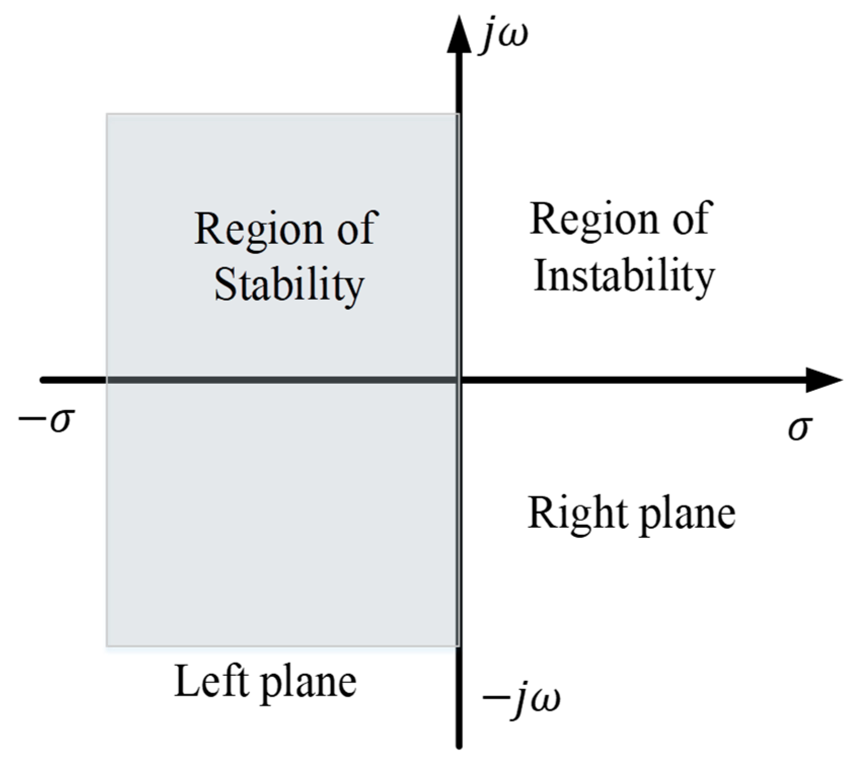
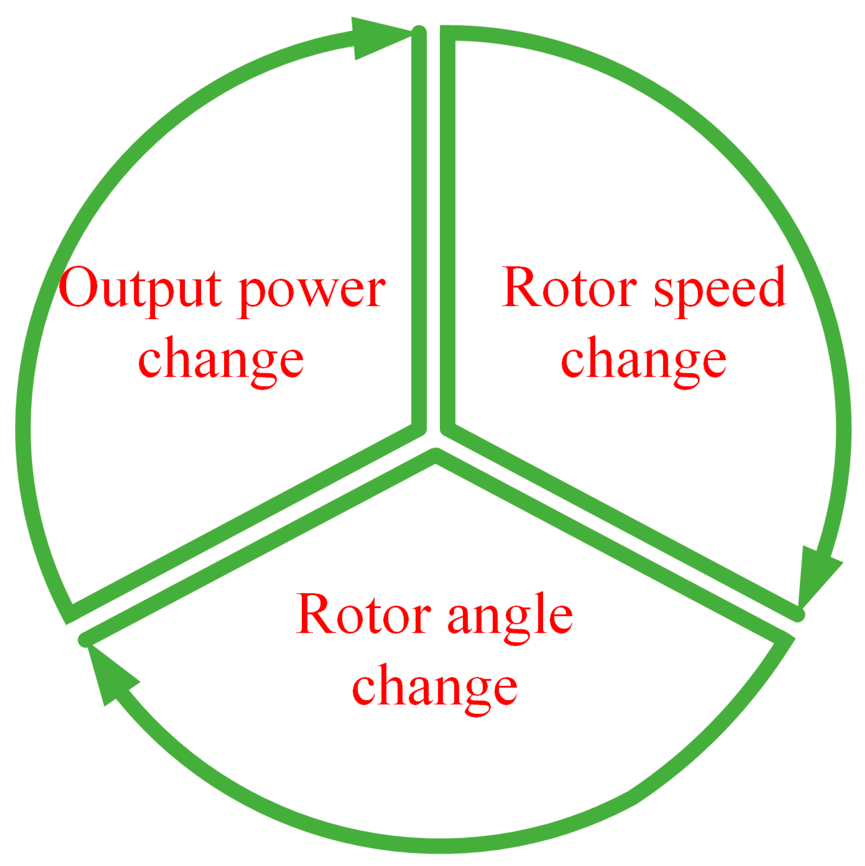
2.1. Power System Stability

The capability of a power grid system to establish restoring forces that are equal to or greater than its disturbing forces, in order to ensure an equilibrium state, is termed power system stability [22,23]. The three basic types of power system stability are voltage stability, frequency stability, and rotor angle stability. In recently integrated power grid systems, converter-driven stability and resonance stability types have been observed [1]. Rotor angle stability involves electromechanical oscillation damping and control, which is a natural phenomenon in synchronous generators. Electromechanical oscillations are caused by imbalances between the electrical and mechanical sections of the synchronous generators, in which the generated (output) power changes with respect to the synchronous generator’s rotor speed and rotor angle. These sequential events involving the rotor speed, rotor angle, and output power account for the electromechanical oscillations in a power grid system. Figure 1 shows this sequential event, which shows that changes in the rotor speed lead to changes in the rotor angle and power output.

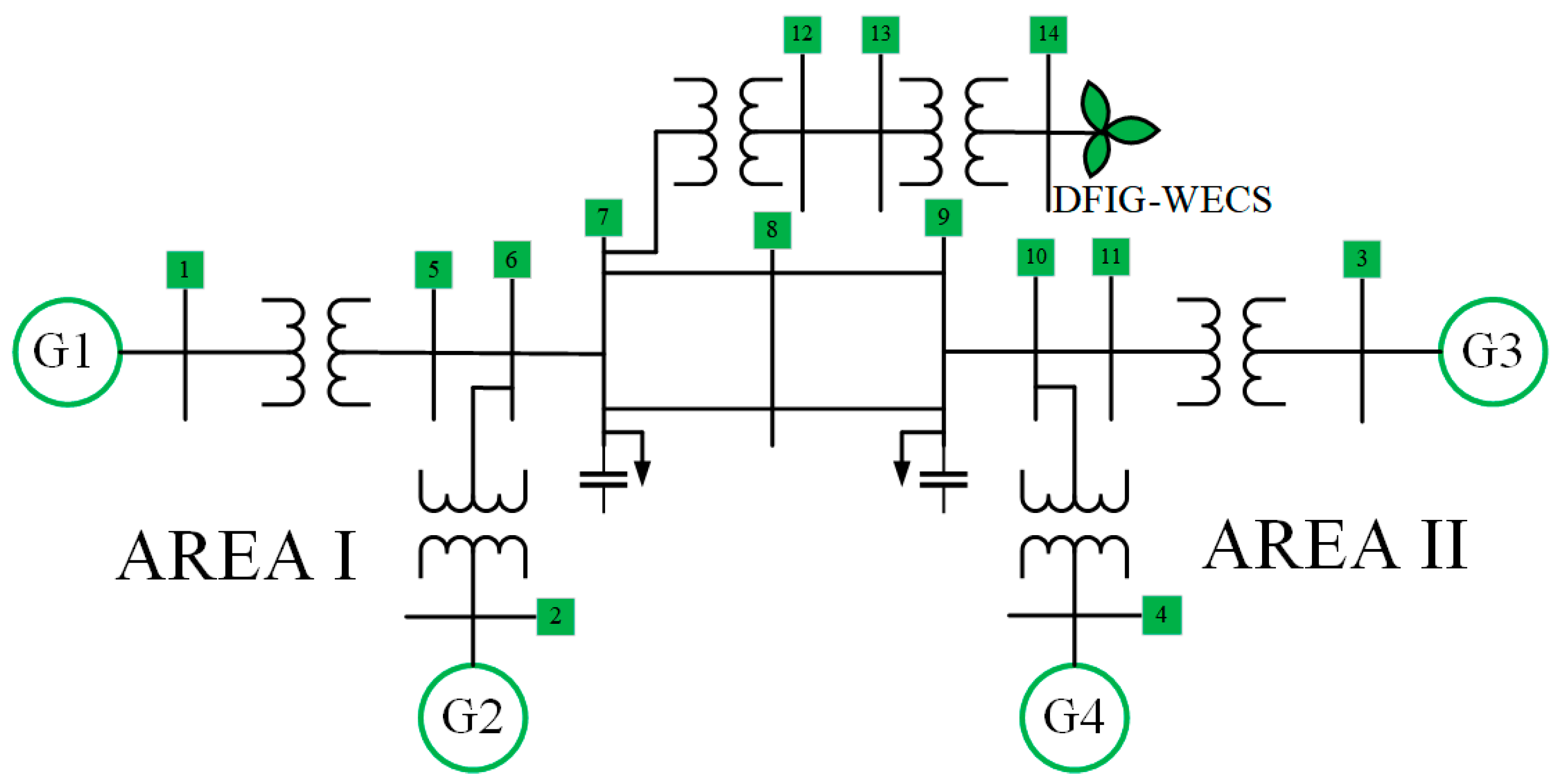
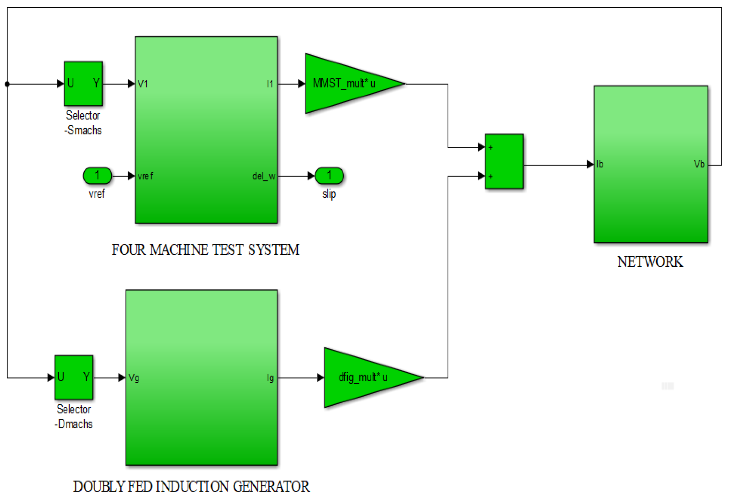
Multimachine Power Test System

This study adopted Kundur’s two-area test system, which is an IEEE benchmark power test system. It consists of four (4) synchronous generators and 11 buses, with two synchronous generators located in each area; bus 3 with synchronous generator number 3 is taken as the reference or slack bus. This power test system was modified to a fourteen (14) bus network by incorporating a DFIG-WECS integrated at bus 14. A single-line diagram of the modified power test system is shown in Figure 2.

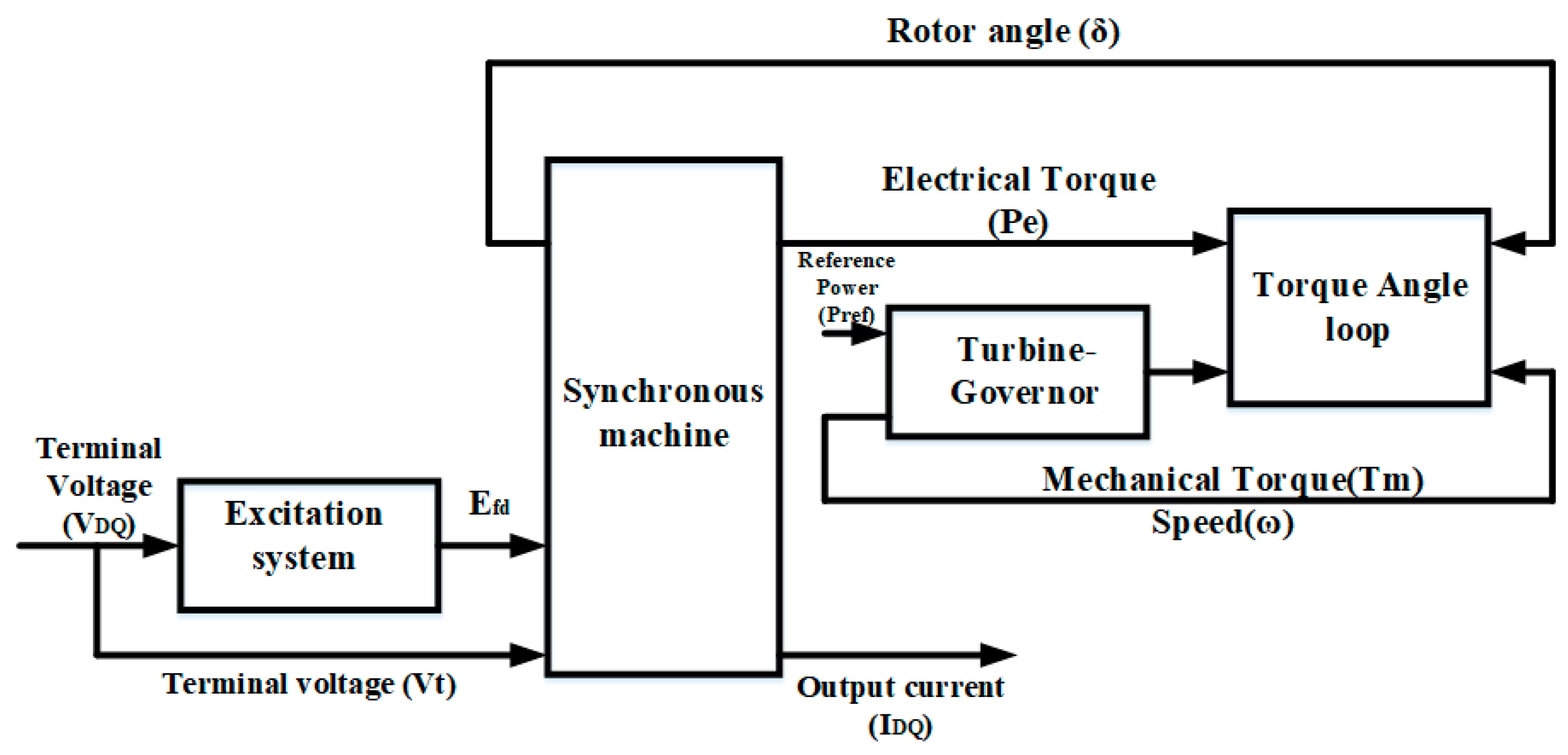
2.2. Conventional Power System

The synchronous generators comprise the conventional power test system, which consists of an excitation system, synchronous generators, turbine/governor system, and torque angle loop. Synchronous generators primarily divide into the stationary part, known as the stator with armature windings, and a rotating part known as the rotor (which can be a salient pole or cylindrical rotor) with field windings. In between these two parts is a small air gap separating them. Symmetries (dq and DQ axis) also exist, which, as recommended by the IEEE, are the reference axes. The reference axes are for easy analysis and representation of the three-phase balanced voltage produced in the synchronous generators. As the rotor rotates with respect to the stator circuits and inductances, time-varying fluxes are induced between the armature stator circuits and the rotor. These time-varying fluxes tend to complicate the analysis and modeling of synchronous generators, but reference axes and symmetries provide a simplified path for easier analysis. Differential algebraic equations (DAEs) are used to describe the conventional power system dynamic models; these DAEs are modeled in Matlab/Simulink, which in turn use ordinary differential equations (ODEs) to obtain the solutions loop. Figure 3 shows a schematic of the solution loop of a conventional power test system.

This schematic diagram can be referred to as the solution loop of the synchronous generator system, which consists of two sides: mechanical and electrical. The torque angle loop represents the mechanical side, while the synchronous generator block represents the electrical side. The governor and an excitation control block are also part of the system. The different parts of the solution loop in Figure 3 were modeled by their DAEs adopted from reference [7]. Equations (1)–(12) were adopted from reference [7] as well. The excitation system is represented in Equation (1) as follows:

$$\frac{d{E}_{fd}}{dt}=\frac{1}{T_a}\left(K_a{V}_{ref}-K_a{E}_t-E_{fd}\right)$$

(1)

In Equation (1), $E_t$ represents the magnitude of the generator voltage, $E_{fd}$ is the voltage in the field winding, $K_a$ represents the static excitation gain, $V_{ref}$ is the reference voltage, and $T_a$ is the static excitation time constant. In the excitation system represented in Equation (1), the field or generator voltage helps to adjust the generator’s excitation system, and in turn, regulates the synchronous generator bus voltage.

The torque angle loop represented in Equation (2) describes the rotor angle and rotor speed change when there is a mismatch between the torques in the synchronous generator mechanical system.

$$\frac{d\delta }{dt}={\omega }_b\left({\omega }_r-{\omega }_s\right)$$

(2)

where $\delta$ represents the rotor angle of the generator, ${\omega }_s$ is the generator’s synchronous speed, ${\omega }_r$ is the generator rotor speed, and ${\omega }_b$ is the base speed value of the generator.

The turbine/governor expressed in Equation (3) helps to regulate the power system’s grid frequency, especially during changes in generation and load balancing; this is achieved by adjusting the generator input torque.

$$\begin{gathered} \frac{d{\omega }_r}{dt}=\frac{1}{2H}\left(T_m-T_e-D\left({\omega }_r-{\omega }_s\right)\right) \\ \frac{d{T}_m}{dt}=\frac{1}{T_g}\left(T_{m2}-T_m-\frac{{\omega }_r-{\omega }_s}{R_{gov}}\right) \end{gathered}$$

(3)

H is the inertia, $T_e$ and $T_m$ are the electrical and mechanical torques, respectively, $D$ is the self-damping, $T_g$ is the time constant of the governor, $R_{gov}$ is the governor droop, and $T_{m2}$ is the generation load reference.

From the solution loop diagram in Figure 3, the synchronous generator itself is the remaining part of the model, and is divided into the electrical torque ($T_e$), the stator current components in the symmetry axis (dq), the symmetry axis (dq) damper coil flux linkage due to the transient EMF in the field, and the symmetry axis (dq) damper flux coil linkage due to the sub-transient EMF in the field. Equation (4) can be used to express the electrical torque. Equation (5) represents the stator current component’s symmetry axis (dq) in the q-axis, and Equation (6) shows it along the d-axis. The symmetry axis (dq) damper coil flux linkage due to transient EMF in the field is described in the q-axis by Equation (7), and in the d-axis by Equation (8). The symmetry axis (dq) damper flux coil linkage due to the sub-transient EMF in the field in the d-axis is expressed in Equation (9) and in the q-axis in Equation (10).

$$T_e=\frac{x_d^{\prime \prime }-x_{ls}}{x_d^{\prime }-x_{ls}}{E}_q^{\prime }{I}_q+\frac{x_d^{\prime }-x_d^{\prime \prime }}{x_d^{\prime }-x_{ls}}{\psi }_{1d}{I}_q+\frac{x_q^{\prime \prime }-x_{ls}}{x_q^{\prime }-x_{ls}}{E}_d^{\prime }{I}_d-\frac{x_q^{\prime }-x_q^{\prime \prime }}{x_q^{\prime }-x_{ls}}{\psi }_{2q}{I}_d+\left(x_q^{\prime \prime }-x_d^{\prime \prime }\right)I_d{I}_q$$

(4)

$$I_q=\frac{R_s}{R_s^2+x_d^{\prime \prime 2}}\left(E_q^{\prime }\frac{x_d^{\prime \prime }-x_{ls}}{x_d^{\prime }-x_{ls}}+{\psi }_{1d}\frac{x_d^{\prime }-x_d^{\prime \prime }}{x_d^{\prime }-x_{ls}}-V_q\right)+\frac{x_d^{\prime \prime }}{R_s^2+x_d^{\prime \prime 2}}\left(E_d^{\prime }\frac{x_q^{\prime \prime }-x_{ls}}{x_q^{\prime }-x_{ls}}-{\psi }_{2q}\frac{x_q^{\prime }-x_q^{\prime \prime }}{x_q^{\prime }-x_{ls}}-V_d\right)$$

(5)

$$I_d=\frac{R_s}{R_s^2+x_d^{\prime \prime 2}}\left(E_d^{\prime }\frac{x_q^{\prime \prime }-x_{ls}}{x_q^{\prime }-x_{ls}}-{\psi }_{2q}\frac{x_q^{\prime }-x_q^{\prime \prime }}{x_q^{\prime }-x_{ls}}-V_d\right)-\frac{x_d^{\prime \prime }}{R_s^2+x_d^{\prime \prime 2}}\left(E_q^{\prime }\frac{x_d^{\prime \prime }-x_{ls}}{x_d^{\prime }-x_{ls}}+{\psi }_{1d}\frac{x_d^{\prime }-x_d^{\prime \prime }}{x_d^{\prime }-x_{ls}}-V_q\right)$$

(6)

$$\frac{d{E}_q^{\prime }}{dt}=\frac{1}{T_{d0}^{\prime }}\left[-E_q^{\prime }+E_{fd}+\left(x_d-x_d^{\prime }\right)\left(I_d+\frac{x_d^{\prime }-x_d^{\prime \prime }}{{\left(x_d^{\prime }-x_{ls}\right)}^2}\left\{{\psi }_{1d}-E_q^{\prime }-I_d\left(x_d^{\prime }-x_{ls}\right)\right\}\right)\right]$$

(7)

$$\frac{d{E}_d^{\prime }}{dt}=\frac{1}{T_{q0}^{\prime }}\left[-E_d^{\prime }+\left(x_q-x_q^{\prime }\right)\left(-I_q+\frac{x_q^{\prime }-x_q^{\prime \prime }}{{\left(x_q^{\prime }-x_{ls}\right)}^2}\left\{-{\psi }_{2q}-E_d^{\prime }+I_q\left(x_q^{\prime }-x_{ls}\right)\right\}\right)\right]$$

(8)

$$\frac{d{\psi }_{2q}}{dt}=\frac{1}{T_{q0}^{\prime \prime }}\left(-{\psi }_{2q}-E_d^{\prime }+I_q\left(x_q^{\prime }-x_{ls}\right)\right)$$

(9)

$$\frac{d{\psi }_{1d}}{dt}=\frac{1}{T_{d0}^{\prime \prime }}\left(-{\psi }_{1d}+E_q^{\prime }+I_d\left(x_d^{\prime }-x_{ls}\right)\right)$$

(10)

where $T_e$ is the electrical torque, and $x_d, x_d^{,},x_d^{,,}$ represent the synchronous generator reactances in the d-axis, and the transient and sub-transient reactances, respectively. $x_q,x_q^{,},x_q^{,,}$ represent the synchronous generator reactances in the q-axis and the transient and sub-transient reactances, respectively. $I_q,I_d$ represent the symmetry (dq) axes of the stator current. ${\psi }_{1d},{\psi }_{2q}$ represent the symmetry (dq) axis of the subtransient EMF flux linkage. $x_{ls}$ gives the leakage armature reactance. $E_d^{\prime },E_q^{\prime }$ represents the symmetry (dq) axis transient EMF flux linkage. $R_s$represents the resistance in the armature, $V_q,V_d$ represent the symmetry (dq) components of the generator terminal voltage, and $T_{d0}^{\prime }, T_{d0}^{\prime \prime }$represent the symmetry (d) axis transient and sub-transient open-circuit time constants, respectively. $T_{q0}^{\prime },T_{q0}^{\prime \prime }$ represent the symmetry (q) axis transient and sub-transient open-circuit time constants, respectively.

To transfer the generated voltage and current from the synchronous generator to the network, transformation frames are required. The transformation frames transform the dq-frames to DQ-frames needed by the network. These transformations are very important, and are explained in detail in reference [7]. The following Equations (11) and (12) represent the voltage and current transformations, respectively:

$$V_q+j{V}_d=\left(V_Q+j{V}_D\right)e^{-j\delta }$$

(11)

$$I_q+j{I}_d=\left(I_Q+j{I}_D\right)e^{-j\delta }$$

(12)

The voltage $V_{qd}$ in the dq frame is transformed using Equation (11) to the DQ frame; likewise, the current from the generator is also transformed using Equation (12) to the network DQ frame. Equations (1)–(12) are coupled together, as shown in the schematic diagram of Figure 3, into a Simulink model that represents the conventional power test system model shown in Figure 4.

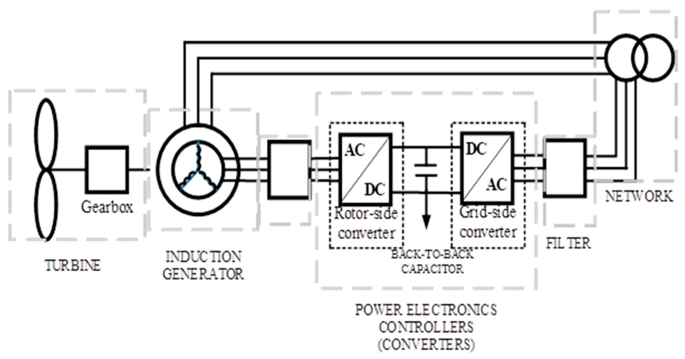
2.3. DFIG-WECS System

The DFIG-WECS consists of a gearbox, turbine, filter, induction generator, and power electronics converters. The power electronics converters include the AC/DC rotor side (machine side) converter and the DC/AC grid side converter. The gearbox converts the wind energy in the turbine to mechanical energy and connects the wind turbine to the induction generator, which utilizes mechanical energy input to generate electricity. The DFIG-WECS is very attractive for wind energy generation because it offers a wide range of variable-speed operations and reactive and active power control. The DFIG-WECS system is shown in Figure 5.

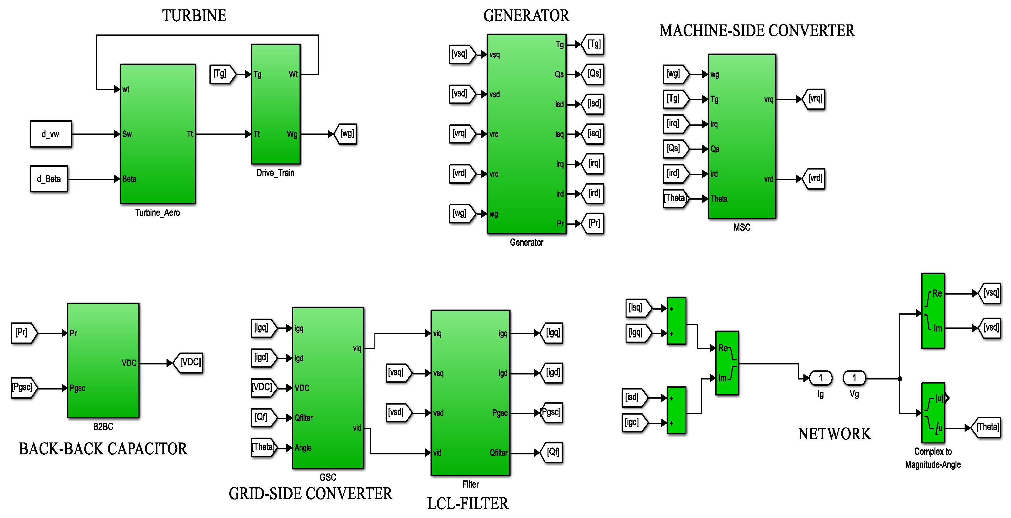
The DFIG-WECS Subsystems

The DFIG-WECS consists of gearbox, turbine, filter, induction generator, and power electronics converters subsystems.

1.

Turbine: It connects the wind speed to the induction generator rotor speed, and it consists of the wind aerodynamic model and the drive train models. The wind aerodynamic model represents the wind power extraction of the rotor, and is expressed in Equation (13); it provides the mechanical power output ($P_t$) fed to the drive train, which depends on the wind speed ($V_w$), blade length of the turbine (R), and power coefficient ($C_p$):

$$P_t=0.5\rho \pi R^2{C}_p\left(\beta ,\lambda \right)V_w^3$$

(13)

where $C_p\left(\beta ,\lambda \right)$ represents the blade power coefficient, which is the part of the wind energy that can be extracted from the turbine; it is a function of $\left(\beta ,\lambda \right)$. Practically, it is usually derived from the performance curve of the turbine obtained from tested field data. However, for simulation purposes, it is represented using numerical approximations, as in Equation (14), which is adapted from reference [7].

$$C_p\left(\beta ,\lambda \right)=0.5176\left(\frac{116}{\lambda +0.08\beta }-\frac{4.06}{1+{\beta }^3}-0.4\beta -5\right) e^{\left(\frac{-21}{\lambda +0.08\beta }+\frac{0.735}{1+{\beta }^3}\right)}+0.0068\lambda$$

(14)

The drive train, on the other hand, uses the mechanical output from the wind aerodynamic model to drive the induction generator, and is represented in Equation (15):

$$\begin{gathered} \frac{d}{dt}{\omega }_g=\frac{1}{2H_g}\left(T_s-T_g\right) \\ {T}_s=K_{tg}{\theta }_{tg}+C_{tg}\frac{d}{dt}{\theta }_g \\ \frac{d}{dt}{\theta }_{tg}=\omega elB\left({\omega }_t-{\omega }_s\right) \\ \frac{d}{dt}{\omega }_t=\frac{1}{2H_t}\left(T_t-T_s\right) \end{gathered}$$

(15)

where subscripts $g,s, \mathrm{and} t$ refer to the generator, shaft, and turbine, respectively. $\omega$ represents the rotor speed of the generator, ${\theta }_{tg}$ is the shaft angle twist of the generator, $H$ is the generator inertia, T represents the drive train shaft stiffness, $C_{tg}$ is the coefficient damping of the drive train, and $\omega elb$ is the electrical base speed.

2.

Induction generator: The generator takes the rotor speed from the turbine and the bus voltage of the generator from the network model as inputs; in turn, it generates the output current and electrical torque. The name DFIG means it has two feeds, the stationary stator part and the rotating rotor part. The stator windings are arranged such that the output stator currents produce a magnetic field that turns the rotor with angular speed in the air gap. The generator adopts the dq reference frames, just like the conventional power grid system. The stator currents in these reference frames are represented by Equation (16):

$$\begin{gathered} \frac{L_s^{\prime }}{\omega elB}\frac{d}{dt}{i}_{sd}=-{\omega }_s{L}_s^{\prime }{i}_{sq}-R_1{i}_{sd}+\frac{e_{sq}^{\prime }}{{\omega }_s{T}_r}+\frac{{\omega }_g{e}_{sd}^{\prime }}{{\omega }_s}+v_{sd}+K_{mrr}{v}_{rd} \\ \frac{L_s^{\prime }}{\omega elB}\frac{d}{dt}{i}_{sq}=-R_1{i}_{sq}+{\omega }_s{L}_s^{\prime }{i}_{sd}+\frac{{\omega }_g{e}_{sq}^{\prime }}{{\omega }_s}-\frac{e_{sd}^{\prime }}{{\omega }_s{T}_r}-v_{sq}+K_{mrr}{v}_{rq} \end{gathered}$$

(16)

where $i_{sd}$ and $i_{sq}$ represent the stator currents in the dq frames, $\omega elB$ is the electrical base speed, the subscripts $g,s$ refer to the generator and shaft, respectively; thus, ${\omega }_s$ is the speed of the generator shaft and ${\omega }_g$ is the generator speed; $L_s^{\prime }$ is the transient stator inductance, $v_{sq,}$ and $v_{sd}$ are the stator voltages in the dq frame, $v_{rd,}$ and $v_{rq}$ are the rotor voltages in the dq frame, $K_{mrr}$ is a transformational parameter derived from Park’s transformation, $e_{sq}^{\prime }$ and $e_{sd}^{\prime }$ represent the generator voltages behind the transient impedances and are represented in Equation (17):

$$\begin{gathered} \frac{1}{{\omega }_s\omega elB}\frac{d}{dt}{e}_{sd}^{\prime }=-R_2{i}_{sq}-\left(1-\frac{{\omega }_g}{{\omega }_s}\right)e_{sq}^{\prime }-\frac{e_{sd}^{\prime }}{{\omega }_s{T}_r}+K_{mrr}{v}_{rq} \\ \frac{1}{{\omega }_s\omega elB}\frac{d}{dt}{e}_{sq}^{\prime }=R_2{i}_{sd}-\frac{e_{sd}^{\prime }}{{\omega }_s{T}_r}+\left(1-\frac{{\omega }_g}{{\omega }_s}\right)e_{sd}^{\prime }-K_{mrr}{v}_{rd} \end{gathered}$$

(17)

where $e_{sq}^{\prime }$ and $e_{sd}^{\prime }$ relate the rotor flux ${\psi }_{rq}$ and ${\psi }_{rd}$, respectively, by Equation (18):

$$\begin{gathered} e_{sd}^{\prime }=-K_{mrr}{\omega }_s{\psi }_{rq} \\ {e}_{sq}^{\prime }=K_{mrr}{\omega }_s{\psi }_{rd} \end{gathered}$$

(18)

The rotor and stator fluxes themselves are given by Equation (19):

$$\begin{gathered} {\psi }_{rq}=L_r{i}_{rq}+L_m{i}_{sq} \\ {\psi }_{rd}=L_r{i}_{rd}+L_m{i}_{sd} \\ {\psi }_{sd}=L_s{i}_{sd}+L_m{i}_{rd} \\ {\psi }_{sq}=L_s{i}_{sq}+L_m{i}_{rq} \end{gathered}$$

(19)

where $L_r, L_m,L_s$ represent the rotor, mutual, and stator inductances, respectively; the generator rotor currents are given by Equation (20):

$$\begin{gathered} i_{rq}=-\left(\frac{e_{sd}^{\prime }}{X_m}\right)-K_{mrr}{i}_{sq} \\ {i}_{rd}=\left(\frac{e_{sq}^{\prime }}{X_m}\right)-K_{mrr}{i}_{sd} \end{gathered}$$

(20)

The generator rotor active and reactive power, the stator active and reactive power, and the electrical torque are described by Equation (21).

$$\begin{gathered} P_r=V_{rq}{i}_{rq}+V_{rd}{i}_{rd} \\ {Q}_r=-V_{rq}{i}_{rd}+V_{rd}{i}_{rq} \\ {P}_s=V_{sq}{i}_{sq}+V_{sd}{i}_{sd} \\ {Q}_s=-V_{sq}{i}_{sd}+V_{sd}{i}_{sq} \end{gathered}$$

(21)

3.

The filter: The filter links the rotor windings of the power grid system. An inductor–capacitor–inductor (LCL) type of filter was used in this study, which is made up of two inductors ($L_i,L_g$), a damping resistor ($R_c$), and a capacitor ($C_f$). The LCL model takes inverter voltage ($v_{iq},v_{id}$) and stator voltage ($v_{sq},v_{sd}$) as inputs, and provides the current injected into the grid through the filter ($i_{gq},i_{gd}$) as outputs. The currents entering the filter are represented by Equation (22):

$$\begin{gathered} \frac{L_i}{{\omega }_b}\frac{d}{dt}i{i}_q=v_{iq}-v_{cq}-\left(R_i+R_c\right)i{i}_q+{\omega }_g{L}_{i}i{i}_d+R_c{i}_{gq} \\ \frac{L_i}{{\omega }_b}\frac{d}{dt}i{i}_d=v_{id}-v_{cd}-\left(R_i+R_c\right)i{i}_d-{\omega }_g{L}_{i}i{i}_q+R_c{i}_{gd} \end{gathered}$$

(22)

The currents exiting the filter are given in Equation (23):

$$\begin{gathered} \frac{L_g}{{\omega }_b}\frac{d}{dt}{i}_{gq}=v_{cq}-v_{sq}-\left(R_g+R_c\right)i_{gq}+\omega L_g{i}_{gd}+R_{c}i{i}_q \\ \frac{L_g}{{\omega }_b}\frac{d}{dt}{i}_{gd}=v_{cd}-v_{sd}-\left(R_g+R_c\right)i_{gd}-\omega L_g{i}_{gq}+R_{c}i{i}_d \end{gathered}$$

(23)

The capacitor voltage of the filter is represented by Equation (24):

$$\begin{gathered} \frac{C_f}{{\omega }_b}\frac{d}{dt}{v}_{cq}=i{i}_q-i_{gq}-\omega C_f{v}_{cd} \\ \frac{C_f}{{\omega }_b}\frac{d}{dt}{v}_{cd}=i{i}_d-i_{gd}+\omega C_f{v}_{cq} \end{gathered}$$

(24)

Lastly, the reactive and active powers exiting the filter are represented by Equation (25):

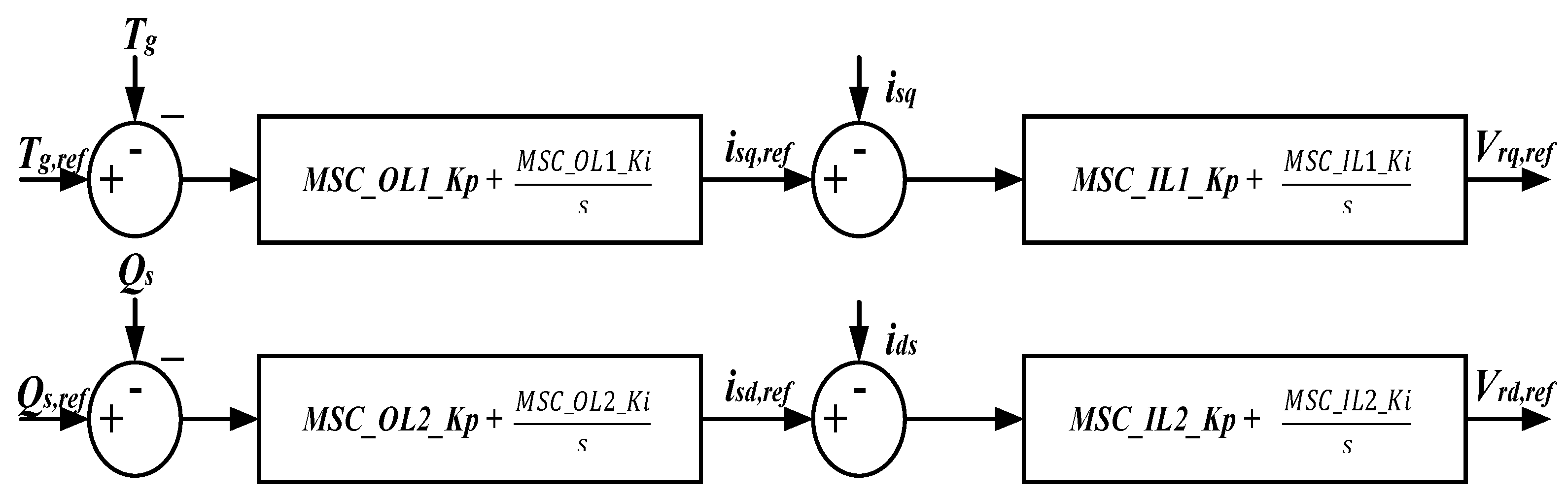
$$\begin{gathered} P_{gsc}=v_{iq}{i}_{iq}+v_{id}{i}_{id} \\ {Q}_{gsc}=-v_{sq}{i}_{gd}+v_{sd}{i}_{gq} \end{gathered}$$

(25)

4.

The power electronics converters: The systems developed so far either represent the mechanical or electrical subsystems of the DFIG power test system. They are quite different from the controllers or converters in the sense that the converters are power electronics converters that contain microcontrollers that are run by some software codes. The power electronics converters include the machine-side and the grid-side converters. The controllers adopted in this study have a simple two cascaded proportional integral (PI) model. The machine-side converter receives voltages, generator rotor speed, and current in the form of electrical signals, and produces corresponding switching signals for the converter. The block diagram of the machine-side converter is shown in Figure 6.

Like the machine-side converter, the grid-side controller also has two cascaded proportional integral (PI) controllers regulating the voltage capacitor and reactive power flow from the grid side at the wind turbine generator bus. Rotor power is transferred to the grid by regulating the capacitor voltage reference value. The block diagram representation of the grid-side converter is shown below in Figure 7.

All of the sub-systems explained so far were coupled together to form the DFIG-WEC system in Matlab/Simulink. The Simulink model is shown in Figure 8.

The conventional multimachine (Kundur’s IEEE) power test system model in Figure 4 and that of the DFIG-WECS in Figure 8 were integrated into a DFIG-WECS IEEE Kundur’s IEEE integrated power grid system, as shown in Figure 9. The bus selector blocks (Smachs and Dmachs) specify the numbers of buses.

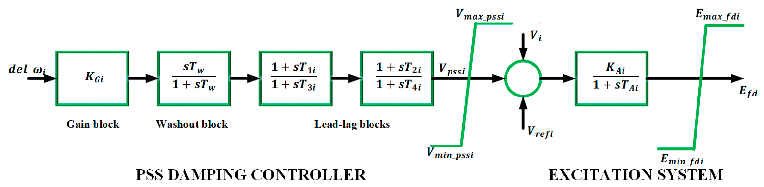
2.4. PSS Damping Controller Design

Electromechanical oscillations occur instantaneously in power grid systems. Hence, automated damping and detection schemes, such as a PSS damping controller, are important in power grid systems. The PSS damping controller, when operated as a compensator for the excitation system, compensates for the input phase lag error between the electrical and mechanical torque components of the generator rotor system [24]. The PSS damping controller, when introduced into a power grid system, also adds an extra input signal to the excitation system of the synchronous generator. It acts as a synchronizing torque that phase locks a synchronized torque signal onto the generator’s speed deviations. This operation improves the stability of the power grid system, and damps the electromechanical oscillations. This study adopted the lead-lag PSS damping controller, as shown in Figure 10, which is mathematically expressed in Equation (26).

$$G_i\left(s\right)=\frac{V_{PSSi}\left(s\right)}{del\_{\omega }_i\left(s\right)}=K_{Gi}\frac{s{T}_W}{\left(1+s{T}_W\right)}\frac{\left(1+s{T}_{1i}\right)\left(1+s{T}_{3i}\right)}{\left(1+s{T}_{2i}\right)\left(1+s{T}_{4i}\right)}$$

(26)

The PSS damping controller consists of the following:

• The control gain $K_{Gi}$: The control gain of the PSS determines the damping introduced by the PSS. The typical range of this value is between 0.1 and 50.
• The washout filter constant $T_W$: The washout filter is a high-pass filter, and is also called a signal washout. It is normally set at 10 s.
• The phase compensators are two lead-lag blocks with parameters $\left(T_{1i},T_{2i},T_{3i},T_{4i}\right)$: The phase compensators determine the phase lag present in the system without the PSS, and then compensates for the phase lag [25].

$V_{PSSi}$represents the output signal of the PSS damping controller, which is the input to the generator excitation system. $del\_{\omega }_i$ represents the PSS signal input, which is the generator rotor’s speed deviation.

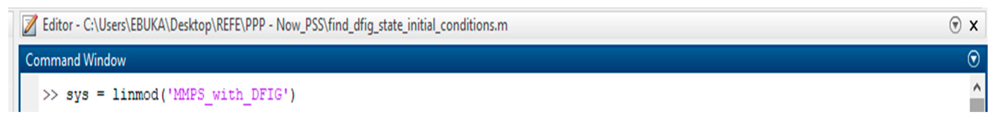
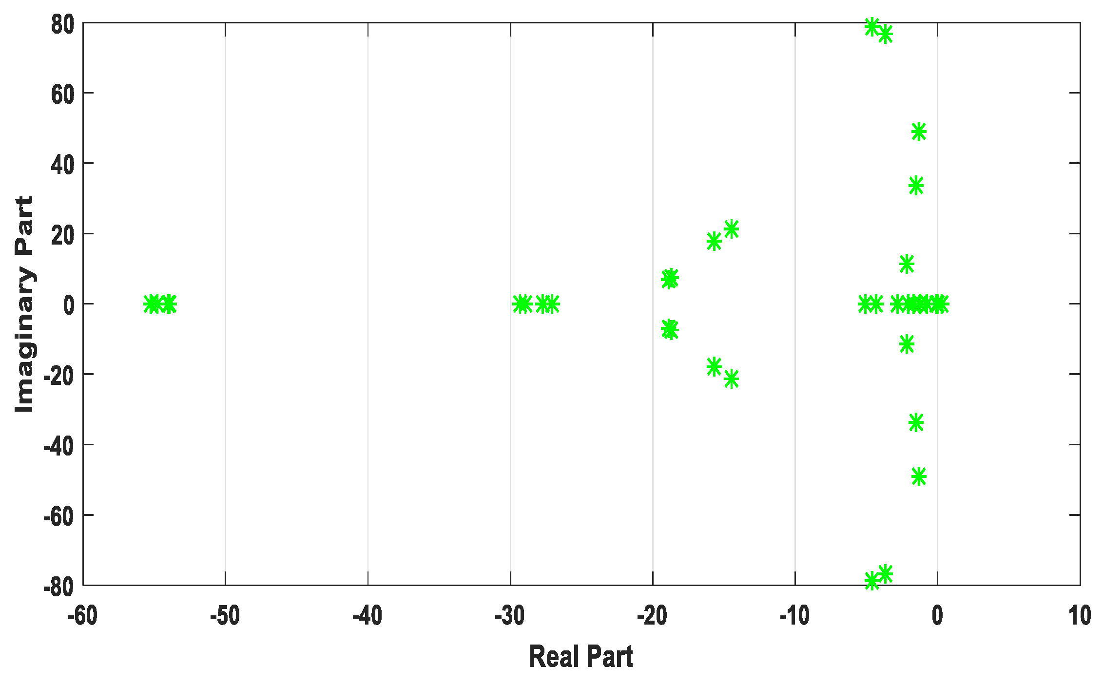
2.5. System Linearization

The power system is composed of various dynamic elements, and is modeled using mathematical DAEs, as shown in the power test system models. These power system DAEs are solved using the ODE solver in MATLAB/Simulink software. It is important to note that the power system model is a non-linear system with constant changes in load flow, power generation, impedances, reactances, and other power flow parameters. However, the PSS damping controller is designed based on the linear control theory; thus, the non-linear power system is linearized about an operating point. For research purposes, a fault was integrated into the Simulink model in Figure 9, by specifying an impedance of zero at Bus 8 from the bus to the ground. A large admittance was added at the diagonal entry that corresponded to the bus in the admittance matrix, and thus the inverse of the new admittance matrix was obtained which gave a post-fault impedance matrix. A screenshot of the program is shown in Figure 11.

In a faulty operating condition, the power system was linearized using a code on the Matlab Integrated Development Environment: [A, B, C, D] = linmod(‘system file name’) or sys = linmod(‘system file name’). Our system file was named MMPS_with_DFIG.slx; however, when inputting the code, the .slx is omitted and represented as sys = linmod(‘MMPS_with_DFIG’). A screenshot of the procedure is shown in Figure 12.

Thus, the non-linear power system was linearized and represented in the state-space form in Equation (27) as follows:

$$\begin{gathered} \Delta \dot{x}=A\Delta x+B\Delta u \\ \Delta y=C\Delta x+D\Delta u \end{gathered}$$

(27)

where $x$ represents the vector state of the system, $u$ is the vector input, and $y$ is the vector output. $A$ is the matrix state, $B$ is the matrix input, $C$ represents the matrix output, and $D$ is the feedforward matrix. The linearized system is shown in Figure 13.

2.6. Objective Function Formulation

The electromechanical oscillation amplitude determines the damping ratio of a system; hence, for the quick attenuation of these oscillations, the PSS damping controller parameters are obtained through optimization. The rotor speed’s deviation error results in electromechanical modes of oscillation. Therefore, to control and damp these electromechanical modes of oscillation, the rotor speed’s deviation error is minimized, which in turn improves the damping ratio. The eigenvalues of state matrix A and its position on a complex S-plane describe the stability of the linear system, which is in the form of Equation (28) as follows:

$${\lambda }_i={\sigma }_i+j{\omega }_i$$

(28)

where ${\sigma }_i$ is the real part that represents damping, and ${\omega }_i$ is the imaginary part that yields the oscillation frequencies of the eigenvalues. Complex conjugate eigenvalues are used to analyze the behavior of the oscillations, and a negative real part results in decreased oscillation, whereas a positive real part results in increased oscillation. In this study, an eigenvalue objective function was defined to damp the electromechanical modes (EMs) and improve damping in the power grid system by moving the eigenvalues to the region of stability (left plane of the complex S-plane). This oscillation behavior is expressed on the complex S-plane, as shown in Figure 14.

The defined objective function yields the PSS controller gains and lead-lag compensator parameters. Equation (29) expresses this objective function, which was adopted from the study in [26].

Minimize J 

 

$$J=minimize \left(max\left\{real\left({\lambda }_i\right)|real \left({\lambda }_i\right) ϵ EMs\right\}\right)+P_C{{\displaystyle \sum }}^{ }\left\{real\left({\lambda }_j\right)|real \left({\lambda }_j\right)>0\right\}$$

(29)

$$EMs=\left\{{\lambda }_k|0<\frac{im\left({\lambda }_k\right)}{2\pi }<5\right\}$$

Subject to $0.001\le K_{pssi}\le 50$ and $0.001\le T_{1i}\le 1,$ $0.02\le T_{2i}\le 1,$ $0.001\le T_{3i}\le 1, 0.02\le T_{4i}\le 1$.

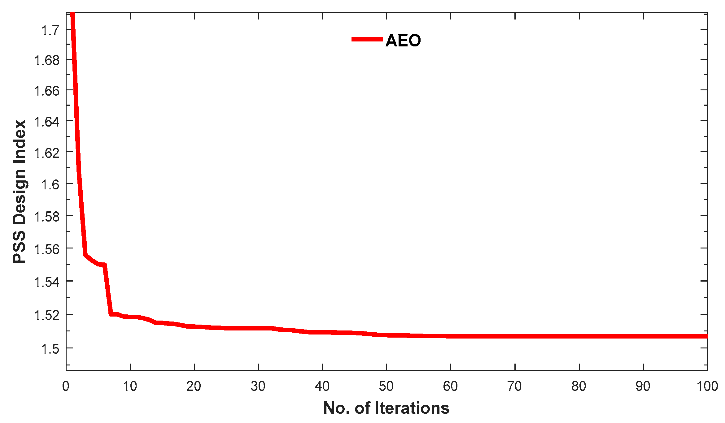
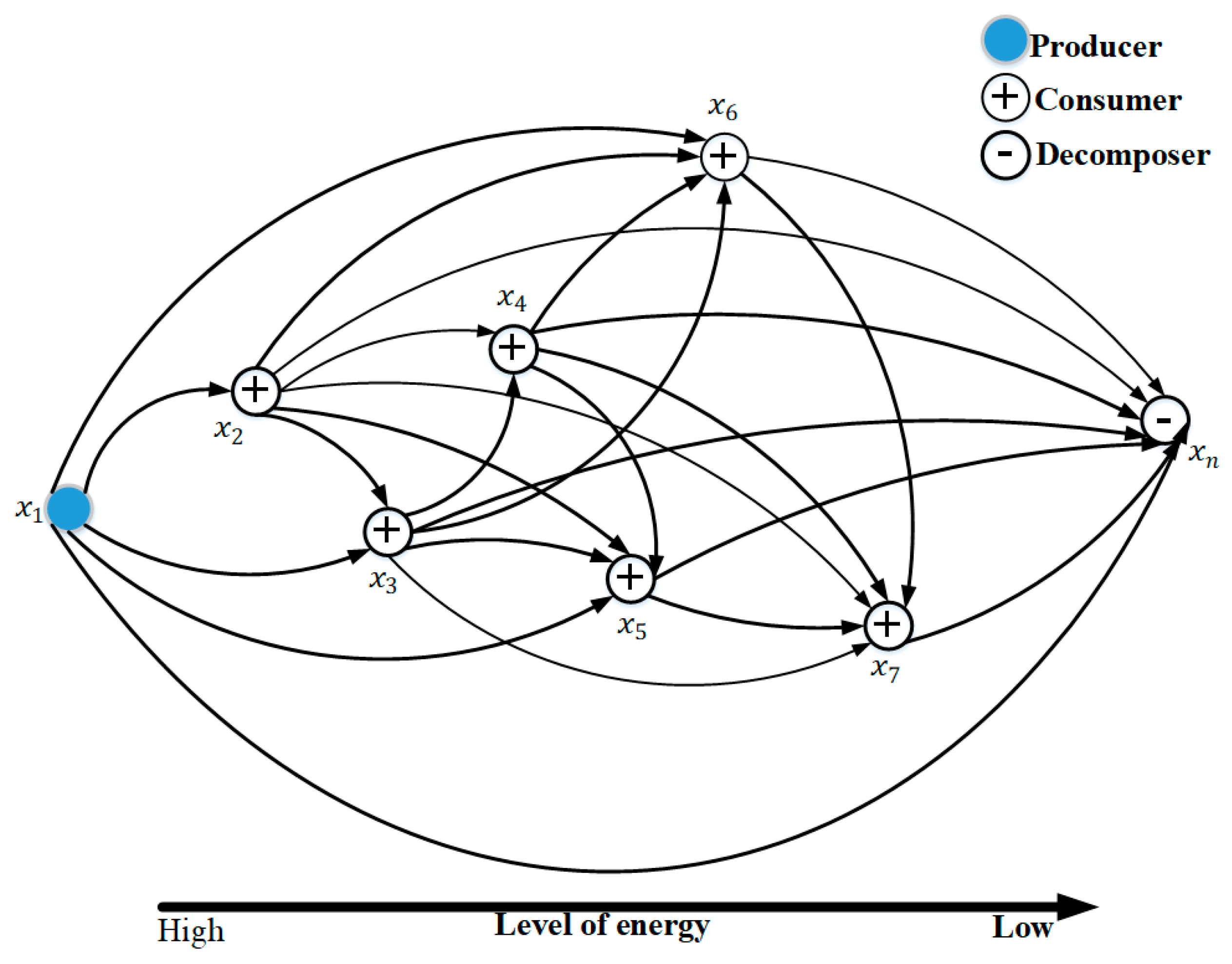
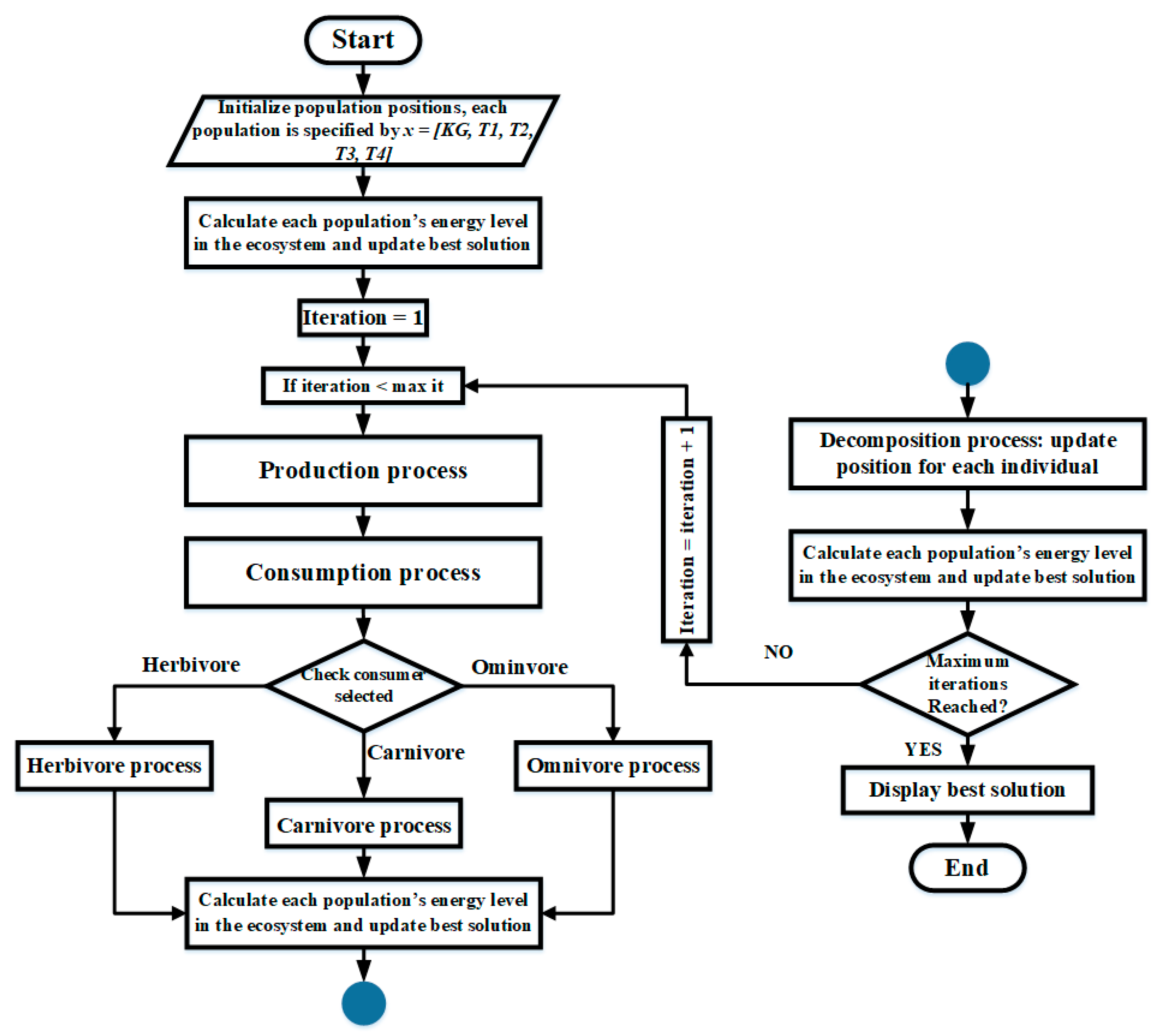
2.7. Artificial Eco-System Optimization (AEO)

The study in reference [27] developed artificial eco-system optimization, which is a metaheuristic algorithm inspired by nature. The AEO algorithm mimics production, consumption, and decomposition operations, which are three unique behaviors of living organisms in an ecosystem. An ecosystem is defined as the complex behavior of living organisms and the inter-relationships in their physical environment within a specific region of space. The two classes of ecosystems are abiotic (sunlight, water, and non-living elements) and biotic (all living elements). As per the metaheuristic algorithm, the AEO search procedure is based on two important features: exploration and exploitation. The production operation enhances the exploitation and exploration balance, the consumption operation improves the exploration ability of the algorithm, and the decomposition process improves exploitation in the algorithm. In a population, every organism’s energy level is accessed based on the defined objective function, and the objective function values are then used to sort individuals in the population into descending order. An individual from the population with the highest objective function value indicates the highest energy level, which forms a minimization problem for optimization. The mathematical modeling of the AEO algorithm is detailed in reference [27]. As previously mentioned, there are three behavioral processes in an ecosystem: production (producer), consumption (consumers are omnivores, carnivores, and herbivores), and decomposition (decomposer). It is assumed that in an ecosystem, there exists only one producer as an individual, and in the population, only one decomposer exists as an individual, as shown in Figure 15. Consumers represent the rest of the population of the ecosystem.

The producer in Figure 15 is the worst individual $x_1$, because it is assumed to have the highest objective function value (high energy), and the best individual is the decomposer ($x_n$), which is assumed to have the lowest objective function value (least energy). The others are consumers, and it is assumed that ($x_2 \mathrm{and} x_3$) are herbivores (animals feeding on plants only), ($x_5 \mathrm{and} x_6$) are omnivores (animals feeding on both plants and animals), and ($x_4 \mathrm{and} x_7$) are carnivores (animals feeding on animals only).

The steps of the AEO algorithm for optimal PSS tuning are as follows:

• Calculate each population’s energy level in the ecosystem via the objective function in Equation (29), and update the best solution.
• Production process: using the production process, update the position for individual $x_1$.
• Consumption process: Each consumer has the same probability for being selected; hence, for individuals $x_2\dots x_7$, their position is updated using the herbivore process if the selected individuals are herbivores. If the selected individual is a carnivore, its position is updated using the carnivore process, and if they were omnivores, the omnivore process is deployed.
• Calculate each population’s energy level in the ecosystem using Equation (29), and update the result as the best solution.
• Decomposition process: Each position of $x_n$ is updated using the production process.
• Calculate each population’s energy level in the ecosystem via the objective function in Equation (29), and update the best solution.
• Repeat steps 3–7 until the maximum number of iterations is reached.

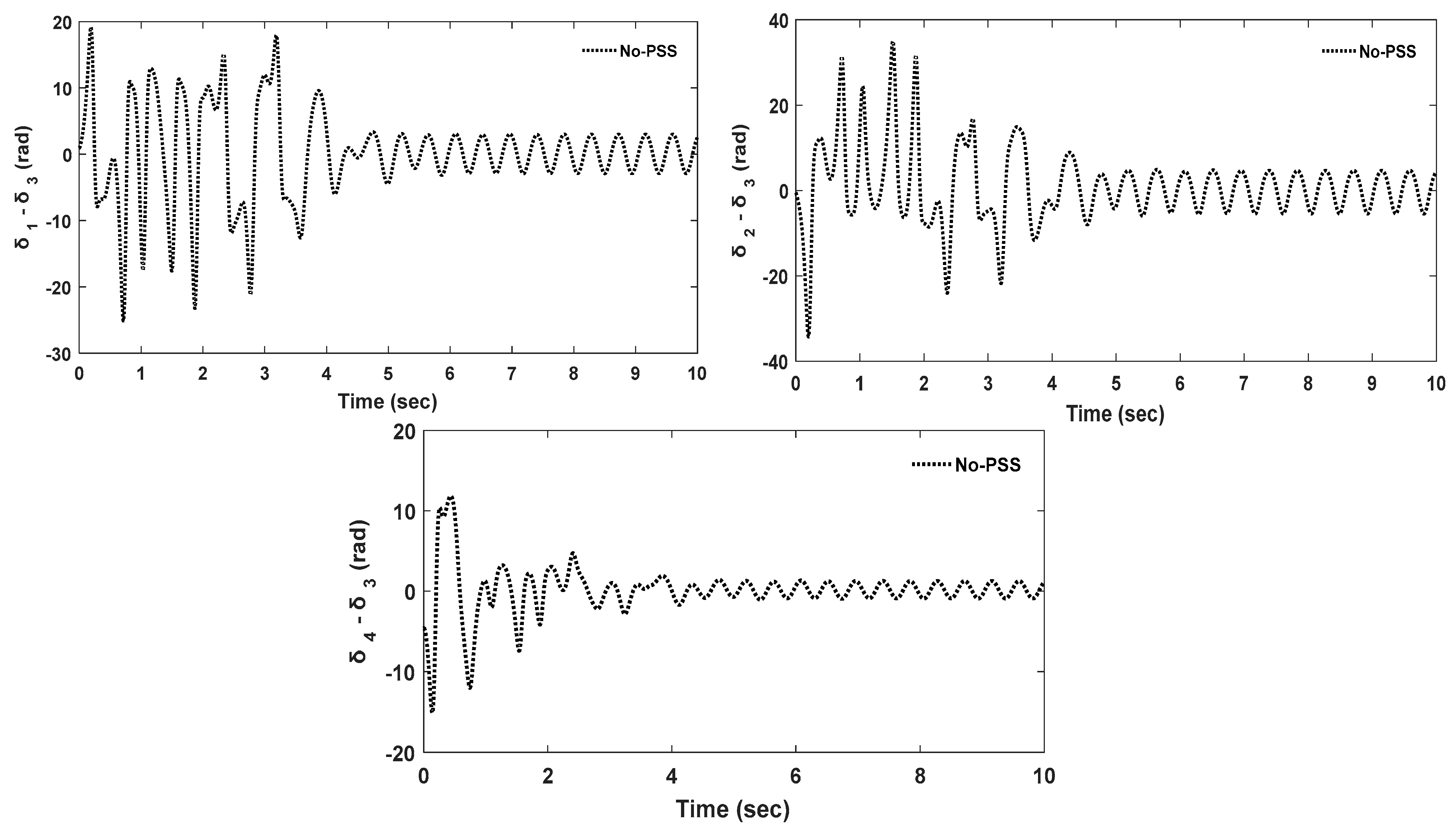
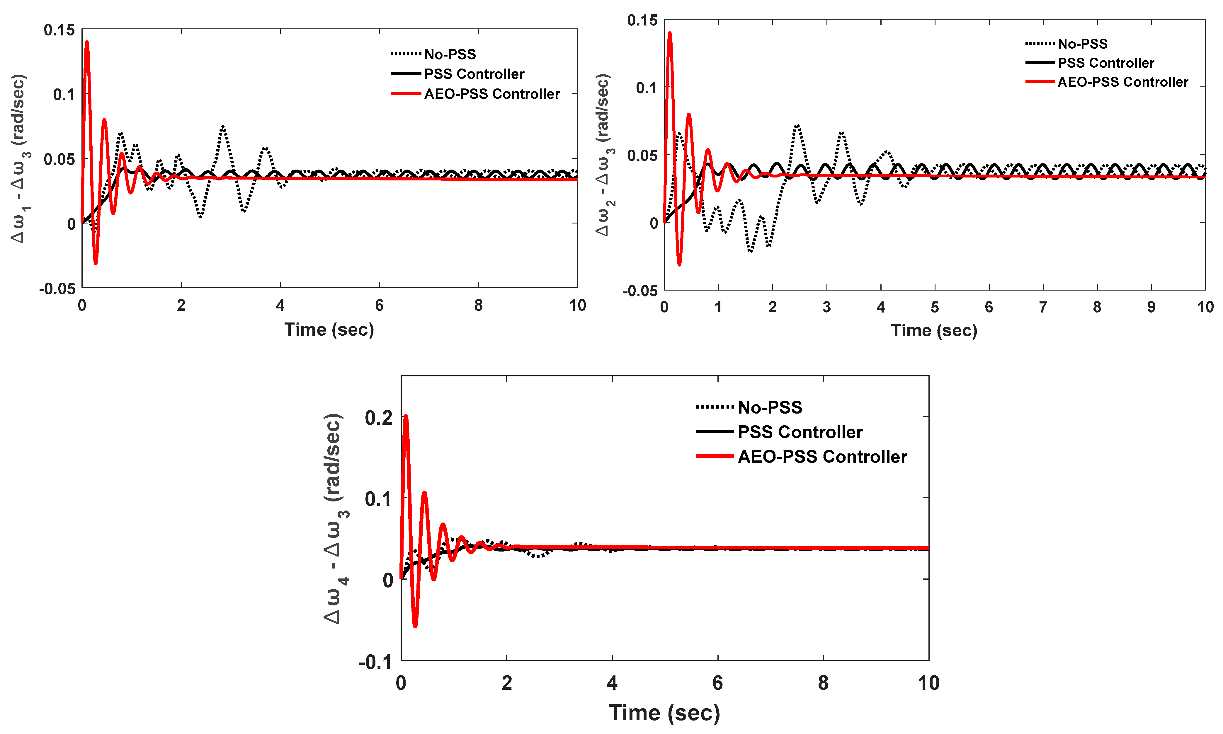
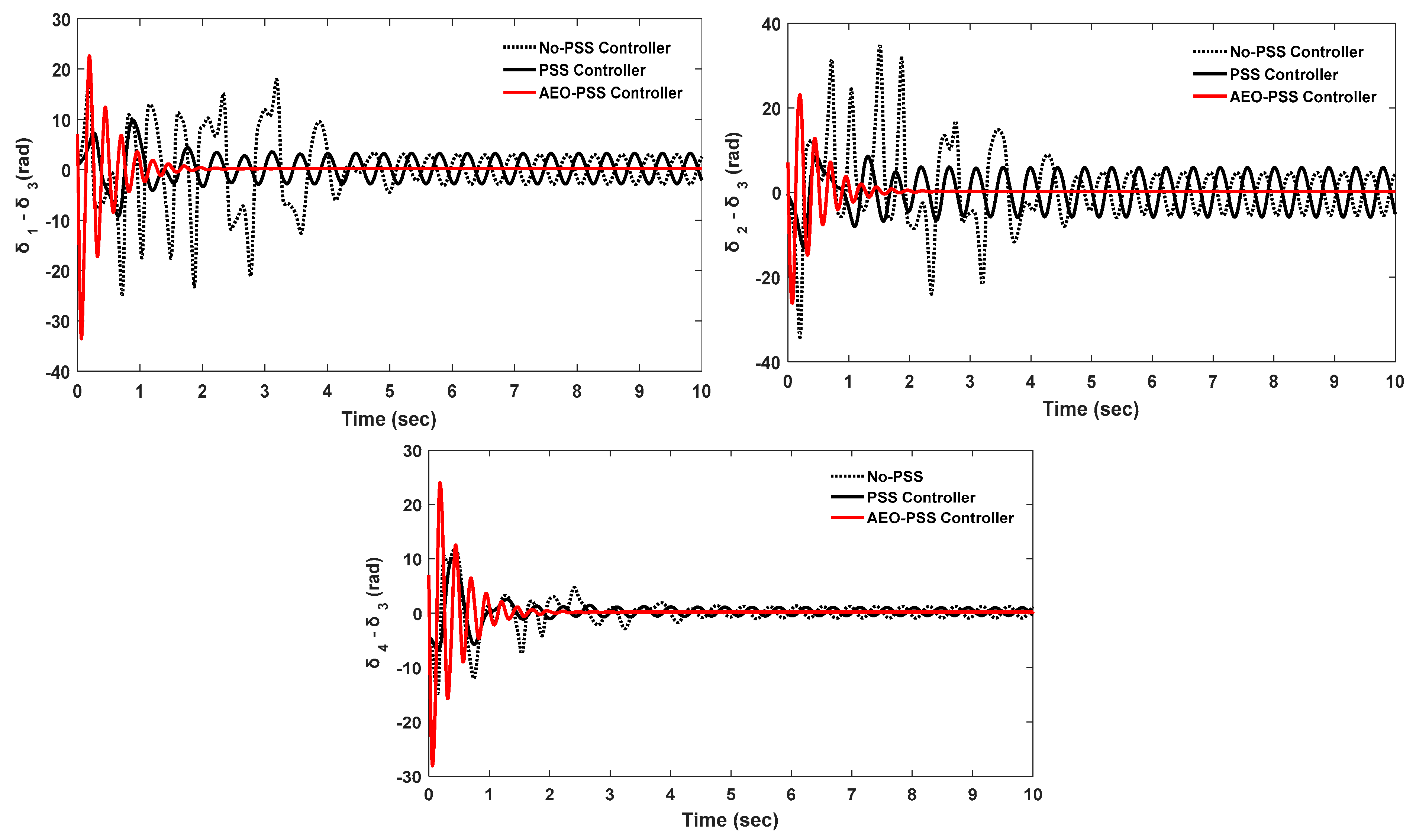
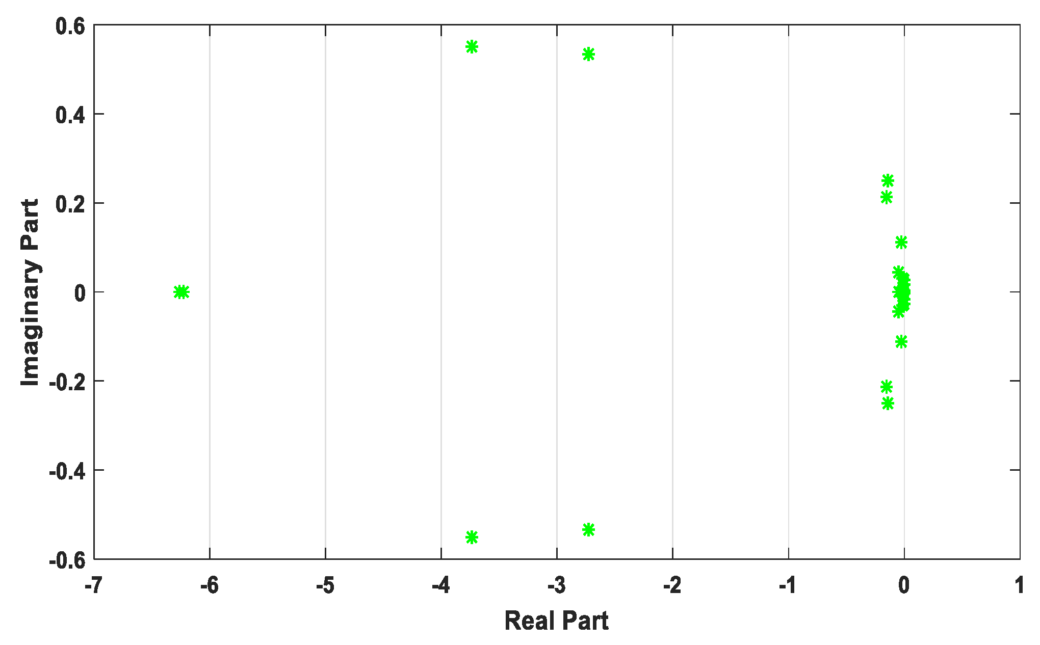
The procedures 3–7 is repeated till maximum iteration or the best/optimal solution is obtained. The flowchart of these steps is shown in Figure 16, while

Table 1. The parameters for the AEO method.

Algorithm	Parameter	Value
AEO	Population size	100
	Maximum size	100
	Number of runs	10
	Producer	$x_1$
	Decomposer	$x_n$
	Consumers	$x_2\dots x_7$

shows the parameters for the AEO optimization method.

3. Results

The IEEE benchmark power test system, as already mentioned, is Kundur’s two-area power test system comprising four (4) synchronous generators and eleven (11) buses. Synchronous generator number 3, which is attached to bus 3, was assumed as the reference/slack bus. The benchmark system was modified to a 14-bus network with the integration of the DFIG-WECS. The bus and line data used for simulation were adopted from reference [7]. Fault was introduced into the multimachine system by specifying a very large admittance at Bus 8. This fault caused electromechanical oscillations in the integrated power grid system. As mentioned in the Introduction section, electromechanical oscillations lead to a sequential event where the generator rotor’s speed change leads to generator rotor angle deviation and output power change. The rotor speed deviations of the generators ($\mathsf{\Delta }\omega$) with the introduction of fault into the multimachine system are shown in Figure 17 with respect to reference bus/generator 3, and are measured in radians per second.

As previously mentioned, rotor speed deviations in the generator lead to generator rotor angle deviations, as shown in Figure 18.

The uncontrolled electromechanical oscillations in the rotor speed and rotor angle of the synchronous generators, as shown in Figure 17 and Figure 18, clearly show that the power test system is unstable. The eigenvalue analysis was performed by linearizing the power test system in its current state-space form, and calculating the eigenvalues of state matrix A and input matrix B. The matrixes can be found at the github link (https:/github.com/Theoodoh/Data-for-Matrices, accessed on 31 March 2024).

Table 2. Eigenvalues of the uncontrolled power system and their corresponding damping ratios.

Mode	Eigenvalue	Damping Ratio
1	$-3.6317\pm 76.9313i$	0.0471
2	$-4.6223\pm 78.5987i$	0.0587
3	$-1.3308\pm 49.1518i$	0.0271
4	$-1.4860\pm 33.4840i$	0.0443
5	$-14.4563\pm 21.0604i$	0.6864
6	$-15.6891\pm 17.8324i$	0.8798
7	$-18.6974\pm 7.4663i$	0.9287
8	$-18.9055\pm 6.9837i$	0.9380
9	$-2.1654\pm 11.1759i$	0.1938
10	$-0.1265\pm 0.1665i$	0.7598
11	$-0.0001\pm 0.0162i$	0.0062
12	$-0.0001\pm 0.0154i$	0.0065
13	$0.0004\pm 0.0009i$	−0.4061

shows these eigenvalues, referred to as electromechanical modes, and their corresponding damping ratios.

A plot of the eigenvalues in Table 1 on the complex S-plane is shown in Figure 19.

In Mode 13 from Table 1, the eigenvalue has a positive real part and when plotted on the complex S-plane in Figure 19, it is positioned on the plane’s right-hand side; which is in the region of instability, as explained and shown in Figure 14 in the objective function formulation. The study in [7] states that even if one of the system eigenvalues appears on the right-hand side of the plane, the system is deemed unstable.

To control these electromechanical oscillations and move the unstable mode to the left side of the plane, PSS damping controllers were installed in synchronous generators 1, 2, and 4 of the power test system. For optimal performance, the AEO algorithm was adopted in designing the damping controllers, and it provided the parameters $\left(K_{Gi}, T_{1i}, T_{2i}, T_{3i}, T_{4i}\right)$. In total, 15 parameters were optimized (i.e., 5 for each PSS damping controller). The obtained parameters are listed in

Table 3. Optimized PSS damping controller parameters.

	${\mathit{K}}_{\mathit{G}\mathit{i}}$	${\mathit{T}}_{\mathbf{1}\mathit{i}}$	${\mathit{T}}_{\mathbf{2}\mathit{i}}$	${\mathit{T}}_{\mathbf{3}\mathit{i}}$	${\mathit{T}}_{\mathbf{4}\mathit{i}}$
$PS{S}_1$	5.1219	0.268	0.055	0.636	0.789
$PS{S}_2$	25.517	0.444	0.594	0.001	0.408
$PS{S}_3$	11.602	0.623	0.297	0.691	0.315

. The optimization curve, which shows the point of convergence to the optimal solution, is shown in Figure 20.

These optimized PSS damping controller parameters were used for time domain simulations in the power test system, in order to control and damp the oscillations. The rotors’ speed responses of the synchronous generators to the installed PSS damping controllers, in comparison with the uncontrolled synchronous generator rotors’ speed responses, are shown in Figure 21.

As already mentioned, controlling the synchronous generator’s rotor speed change leads to control of the synchronous generator’s rotor angle, as explained in the sequential events of electromechanical oscillations; thus, with control over the rotor speeds of the synchronous generators, the rotor angles of the synchronous generators are controlled as well. Figure 22 shows a comparison of the rotor angles of the controlled and uncontrolled synchronous generators.

To further improve the damping and control of electromechanical oscillations, the power test system was again linearized in its current state-space form described in Equation (27); state matrix A and input matrix B, which can be accessed via the github link (https://github.com/Theoodoh/Data-for-Matrices, accessed on 31 March 2024), were calculated, as well as the eigenvalues that show the state of the system.

Table 4. Eigenvalues of the controlled power system and their corresponding damping ratios.

Mode	Eigenvalue	Damping Ratio
1	$-3.7398\pm 0.5512i$	0.9893
2	$-2.7398\pm 0.5338i$	0.9813
3	$-0.1437\pm 0.2487i$	0.5004
4	$-0.1530\pm 0.2133i$	0.5829
5	$-0.0465\pm 0.0433i$	0.7313
6	$-0.0217\pm 0.1118i$	0.1902
7	$-0.0138\pm 0.0320i$	0.3958
8	$-0.0526\pm 0.0014i$	0.9997
9	$-0.0086\pm 0.0263i$	0.3108
10	$-0.0060\pm 0.0176i$	0.3226
11	$-0.0110\pm 0.0118i$	0.6819
12	$-0.0197\pm 0.0008i$	0.9991
13	$-0.0013\pm 0.0017i$	0.6075

shows the dominant eigenvalues and their corresponding damping ratios.

As seen from Table 4, all of the eigenvalues have negative real parts, which means that they all appear on the plane’s left-hand side, indicating that the power test system is stable. In particular, Mode 13 was moved to the plane’s left-hand side compared with what is shown in Table 2, with a damping ratio of 0.6075. The eigenvalue plots in Table 4 are shown in Figure 23.

4. Discussion

This study presented the integration of DFIG-WECS into Kundur’s two-area power test system, which is an IEEE benchmark test system. The two power test systems were modeled separately using DAEs, and the modeling is explained in detail in study [7], including the power flow programs and bus and line data for initialization. For the integration of the DFIG-WECS, bus 7 was extended to buses 12, 13, and 14. The DFIG-WECS was connected at bus 14, modifying the two-area test system into a 14-bus network. On the integrated system, a fault was injected into bus 8, which is the mid-bus of the two-area test system, by specifying a large admittance on the bus and calculating for the post-fault admittance matrix. In a faulty system electromechanical oscillation is evident from Figure 17 and Figure 18, and also in Table 2, which shows the uncontrolled eigenvalues. Mode 13 was identified as an unstable mode with a negative damping ratio, meaning that there was continuous oscillation in the power test system. Then, the PSS damping controller was introduced to control and damp the oscillation. Since the PSS works based on linear control theory, the power system was linearized and the PSS designed with the AEO algorithm was introduced into generators 1, 2, and 4. In all, 15 PSS parameters were optimized, 5 parameters for each PSS damping controller. Upon performing simulations with the optimized PSS values, the stability of the power system improved through an attenuating oscillation; moreover, all of the eigenvalues, particularly mode 13 that was identified as an unstable mode with a negative damping ratio, improved to a positive damping ratio. The aim of the study, which was according to study [7], resulted in the achievement of a stable system when all of the eigenvalues appeared on the left side of the complex S-plane, as shown in Figure 23 and Table 4 (all of the eigenvalues had negative real parts). This research also shows that even if one eigenvalue appears on the right side of the complex S-plane, the system is deemed unstable. See Figure 19 and Table 2 (Mode 13 has a positive real part).

5. Conclusions

Damping and controlling electromechanical oscillations in an integrated Kundur’s two-area network with a DFIG-WECS was presented. Upon integrating the DFIG-WECS system and introducing a fault into the power test system, eigenvalue analysis showed that the system became unstable. Mode 13, with a damping ratio of −0.4061, was identified as the unstable mode. PSS damping controllers that were designed using the artificial ecosystem optimization (AEO) algorithm were able to control electromechanical oscillations by controlling synchronous generator rotor speeds and rotor angle deviations. Again, eigenvalue analysis proved that the system became stable by moving unstable Mode 13 to the region of stability with a damping ratio of 0.6075. This study can further be improved by integrating the DFIG-WECS into a larger IEEE benchmark power test system like the thirty-nine (39) bus network known as the New England. FACTS devices such as a static compensator (STATCOM), interline power flow controller (IPFC), static VAR compensator (SVC), and a unified power flow controller (UPFC) with power oscillation dampers (PODs) can also be introduced to the system. Power system stabilizer (PSS), and FACTS device can be combined and introduced into the system to improve electromechanical oscillation damping. Fuzzy logic damping controllers and neural networks, such as the neuro-fuzzy controller, can also be introduced into the system.

References

1. Elkasem, A.H.A.; Kamel, S.; Khamies, M.; Kabalci, E.; Shahinzadeh, H. Frequency stability enhancement of hybrid multi-area power grid considering high renewable energy penetration using TID controller. In Proceedings of the 2022 4th Global Power, Energy and Communication Conference (GPECOM), Nevsehir, Turkey, 14–17 June 2022; pp. 322–327. [Google Scholar]
2. Sabo, A.; Kolapo, B.Y.; Odoh, T.E.; Dyari, M.; Abdul Wahab, N.I.; Veerasamy, V. Solar, Wind and Their Hybridization Integration for Multi-Machine Power System Oscillation Controllers Optimization: A Review. Energies 2023, 16, 24. [Google Scholar] [CrossRef]
3. Bhukya, J.; Mahajan, V. The controlling of the DFIG based on variable speed wind turbine modeling and simulation. In Proceedings of the 2016 IEEE 6th International Conference on Power Systems (ICPS), New Delhi, India, 4–6 March 2016; pp. 1–6. [Google Scholar] [CrossRef]
4. Bhukya, J.; Mahajan, V. Optimization of controllers parameters for damping local area oscillation to enhance the stability of an interconnected system with wind farm. Int. J. Electr. Power Energy Syst. 2020, 119, 105877. [Google Scholar] [CrossRef]
5. Rawal, M.; Nauityal, D.C.; Rawat, M.S. Analysis of small signal stability in DFIG integrated power system. In Proceedings of the 2021 International Conference on Advances in Electrical, Computing, Communication and Sustainable Technologies (ICAECT), Bhilai, India, 19–20 February 2021. [Google Scholar] [CrossRef]
6. Geng, H.; Xi, X.; Yang, G. Small-signal stability of power system integrated with ancillary-controlled largescale DFIG-based wind farm. IET Renew. Power Gener. 2017, 11, 1191–1198. [Google Scholar] [CrossRef]
7. Kunjumuhammed, L.; Kuenzel, S.; Pal, B.C. Simulation of Power System with Renewables; Academic Press: Cambridge, MA, USA, 2019; ISBN 0128112549. [Google Scholar]
8. Essallah, S.; Bouallegue, A.; Khedher, A. Integration of automatic voltage regulator and power system stabilizer: Small-signal stability in DFIG-based wind farms. J. Mod. Power Syst. Clean Energy 2019, 7, 1115–1128. [Google Scholar] [CrossRef]
9. Sabo, A.; Odoh, T.E.; Shahinzadeh, H.; Azimi, Z.; Moazzami, M. Implementing Optimization Techniques in PSS Design for Multi-Machine Smart Power Systems: A Comparative Study. Energies 2023, 16, 2465. [Google Scholar] [CrossRef]
10. Sabo, A.; Abdul Wahab, N.I.; Othman, M.L.; Mohd Jaffar, M.Z.A.; Beiranvand, H. Optimal design of power system stabilizer for multimachine power system using farmland fertility algorithm. Int. Trans. Electr. Energ Syst. 2020, 30, e12657. [Google Scholar] [CrossRef]
11. Sabo, A.; Wahab, N.I.A.; Othman, M.L.; Jaffar, M.Z.A.M.; Beiranvand, H. Farmland fertility optimization for designing of interconnected multi-machine power system stabilizer. Appl. Model. Simul. 2020, 4, 183–201. [Google Scholar]
12. Sabo, A.; Abdul Wahab, N.I.; Othman, M.L.; Mohd Jaffar, M.Z.A.; Beiranvand, H.; Acikgoz, H. Application of a neuro-fuzzy controller for single machine infinite bus power system to damp low-frequency oscillations. Trans. Inst. Meas. Control 2021, 43, 3633–3646. [Google Scholar] [CrossRef]
13. He, P.; Zheng, M.; Li, Z.; Fang, Q.; Wu, X. Research on improving low frequency oscillation characteristics of wind power system with DFIG-PSS-VI. E3S Web Conf. 2021, 252, 2001. [Google Scholar] [CrossRef]
14. Farah, A. A new design method of PSS for power system including DFIG-based wind turbines. In Proceedings of the 2021 12th International Renewable Engineering Conference (IREC), Amman, Jordan, 14–15 April 2021; pp. 1–6. [Google Scholar] [CrossRef]
15. Prasad, D.K. Analysis of Small Signal and Transient Stability under the Penetration of DFIG Integrated Wind Energy Conversion System. In Proceedings of the 2019 International Conference on Electrical, Electronics and Computer Engineering (UPCON), Aligarh, India, 8–10 November 2019; pp. 1–6. [Google Scholar]
16. Kamel, O.M.; Abdelaziz, A.Y.; Zaki Diab, A.A. Damping Oscillation Techniques for Wind Farm DFIG Integrated into Inter-Connected Power System. Electr. Power Compon. Syst. 2020, 48, 1551–1570. [Google Scholar] [CrossRef]
17. Shah, N.N.; Joshi, S.R. Utilization of DFIG-based wind model for robust damping of the low frequency oscillations in a single SG connected to an infinite bus. Int. Trans. Electr. Energy Syst. 2019, 29, e2761. [Google Scholar] [CrossRef]
18. Du, C.; Han, Y.; Li, S. Continuous twisting damping Control of DFIG-Based Wind Farm to Improve Interarea Oscillation Damping. In Proceedings of the 2021 China Automation Congress (CAC), Beijing, China, 22–24 October 2023; pp. 5432–5437. [Google Scholar] [CrossRef]
19. Tan, A.; Tang, Z.; Sun, X.; Zhong, J.; Liao, H.; Fang, H. Genetic Algorithm-Based Analysis of the Effects of an Additional Damping Controller for a Doubly Fed Induction Generator. J. Electr. Eng. Technol. 2020, 15, 1585–1593. [Google Scholar] [CrossRef]
20. Dhami, N.; Bhadu, M.; Bishnoi, S.K.; Sharma, K.G. Impact of PSS Tuning Methods on Grid Connected DFIG System. pp. 1–7. Available online: https://ssrn.com/abstract=3314844 (accessed on 2 April 2024).
21. Hannan, M.A.; Islam, N.N.; Mohamed, A.; Lipu, M.S.H.; Ker, P.J.; Rashid, M.M.; Shareef, H. Artificial intelligent based damping controller optimization for the multi-machine power system: A review. IEEE Access 2018, 6, 39574–39594. [Google Scholar] [CrossRef]
22. Kundur, P.; Paserba, J.; Ajjarapu, V.; Andersson, G.; Bose, A.; Canizares, C.; Hatziargyriou, N.; Hill, D.; Stankovic, A.; Taylor, C. Definition and classification of power system stability IEEE/CIGRE joint task force on stability terms and definitions. IEEE Trans. Power Syst. 2004, 19, 1387–1401. [Google Scholar]
23. Saadat, H. Power System Analysis, 2nd ed.; McGraw Hill Higher Education: New York, NY, USA, 2009. [Google Scholar]
24. Ekinci, S.; İzci, D.; Hekimoğlu, B. Implementing the Henry Gas Solubility Optimization Algorithm for Optimal Power System Stabilizer Design. Electrica 2021, 21, 250–258. [Google Scholar] [CrossRef]
25. Ekinci, S.; Demiroren, A.; Hekimoglu, B. Parameter optimization of power system stabilizers via kidney-inspired algorithm. Trans. Inst. Meas. Control 2019, 41, 1405–1417. [Google Scholar] [CrossRef]
26. Beiranvand, H.; Rokrok, E. General relativity search algorithm: A global optimization approach. Int. J. Comput. Intell. Appl. 2015, 14, 1550017. [Google Scholar] [CrossRef]
27. Zhao, W.; Wang, L.; Zhang, Z. Artificial ecosystem-based optimization: A novel nature-inspired meta-heuristic algorithm. Neural Comput. Appl. 2020, 32, 9383–9425. [Google Scholar] [CrossRef]
Figure 1. Sequential events in electromechanical oscillations.
Energies 17 01841 g001
Figure 2. Two-area (Kundur’s two-area IEEE) power test system single-line diagram augmented by the DFIG-WECS. 1–14 in the Figure represents the buses (bus bars) in the power grid system.
Energies 17 01841 g002
Figure 3. Schematic diagram of the solution loop for a conventional power test system.
Energies 17 01841 g003
Figure 4. Simulink model of the solution loop for the conventional power test system.
Energies 17 01841 g004
Figure 5. DFIG-WECS system.
Energies 17 01841 g005
Figure 6. Block diagram of the machine-side converter.
Energies 17 01841 g006
Figure 7. Block diagram of the grid-side converter.
Energies 17 01841 g007
Figure 8. Simulink model of the DFIG-WECS system.
Energies 17 01841 g008
Figure 9. Simulink model of the integrated conventional multimachine and DFIG-WECS power test systems.
Energies 17 01841 g009
Figure 10. PSS damping controller system.
Energies 17 01841 g010
Figure 11. Adding fault into the system.
Energies 17 01841 g011
Figure 12. Matlab linearization process.
Energies 17 01841 g012
Figure 13. The linearized system.
Energies 17 01841 g013
Figure 14. The complex S-plane.
Energies 17 01841 g014
Figure 15. AEO optimization process.
Energies 17 01841 g015
Figure 16. Flowchart of the AEO process.
Energies 17 01841 g016
Figure 17. Time domain simulation results of uncontrolled rotor speed deviations of the synchronous generators.
Energies 17 01841 g017
Figure 18. Time domain simulation results of uncontrolled rotor angle deviations of the synchronous generators.
Energies 17 01841 g018
Figure 19. Uncontrolled oscillations eigenvalue plot on the complex S-plane.
Energies 17 01841 g019
Figure 20. Optimization curve for the AEO-PSS damping controller.
Energies 17 01841 g020
Figure 21. Time domain simulations of the controlled synchronous generators’ rotor speed deviations.
Energies 17 01841 g021
Figure 22. Time domain simulations of the controlled synchronous generators’ rotor angle deviations.
Energies 17 01841 g022
Figure 23. Controlled power system eigenvalues plotted on the complex S-plane.
Energies 17 01841 g023