The Prediction of Medium- and Long-Term Trends in Urban Carbon Emissions Based on an ARIMA-BPNN Combination Model

Abstract

Urban carbon emissions are an important area for addressing climate change, and it is necessary to establish scientific and effective carbon emission prediction models to formulate reasonable emission reduction policies and measures. In this paper, a novel model based on Lasso regression, an ARIMA model, and a BPNN is proposed. Lasso regression is used to screen the key factors affecting carbon emissions, and the ARIMA model is used to extract the linear components of the carbon emission sequences, while the BPNN is used to predict the residuals of the ARIMA model. The final result is the sum of that from the ARIMA model and the BPNN. The carbon peak, carbon neutralization time, and emissions were analyzed under different scenarios. Taking Suzhou City as an example, the results show that the electricity consumption of the whole population is one of the key drivers of carbon emissions; the carbon emission prediction accuracy and stability of the ARIMA-BPNN combined model are better than those of the single model, which improves the reliability as well as the accuracy of the model’s prediction. However, under the constraints of the current policies, the goal of achieving carbon peaking by 2030 in Suzhou City may not be realized as scheduled. This novel carbon emission prediction model built was validated to provide a scientific basis for low-carbon urban development. This study presents an important reference value for predicting carbon emissions and formulating emission reduction measures in other cities.

1. Introduction

With the rapid development of the global economy, human activities have brought about more and more negative effects on the ecological environment, especially greenhouse gas emissions, leading to the intensification of global climate change [1]. Carbon dioxide is one of the most important greenhouse gases [2], and its emissions are closely related to global warming. Therefore, controlling and reducing carbon dioxide emissions are some important actions for dealing with climate change. China proposed the dual carbon goal of peaking by 2030 and achieving neutrality by 2060 in 2020. Cities are highly concentrated areas in terms of population and the economy and are one of the main sources of energy consumption and carbon dioxide emissions [3]. Prediction and analysis of carbon dioxide emissions in cities are essential to formulate reasonable emission reduction policies and measures and improve the level of low-carbon development in cities.

At present, the research on carbon emission prediction mainly focuses on the factors affecting carbon emissions and the methods of carbon emission prediction. The selection of appropriate influencing factors is the foundation for establishing carbon emission prediction models. The current research mostly considers factors such as population size, economic scale, energy structure, energy intensity, industrial structure, and urbanization level to establish carbon emission prediction models, including carbon emission assessments globally across six continents (Europe, North America, South America, Asia, Africa, and Oceania) [4] and in the Beijing–Tianjin–Hebei region [5], as well as Guangdong Province [6]. Meanwhile, the land use change rate, forest protection situation, biomass energy utilization efficiency, transportation mode, and renewable energy utilization rate were taken into account for Brazil’s carbon emissions by Pedreira [7]. Chen et al. [8] added the proportion of R&D investment as a variable affecting the carbon emissions in Beijing, while Mitchell et al. [9] considered the impact of automobile usage intensity, public transportation usage intensity, and climate factors such as season, temperature, and wind speed on the carbon emissions in 12 cities in the United States. Wu and Zhang [10] also examined the impact of foreign direct investment (FDI) on carbon emission efficiency. Gray correlation analysis was used to screen for factors such as energy consumption, industrial structure (proportion of tertiary industries), and dependence on foreign trade to predict China’s carbon emissions by Dong and Li [11]. However, this method cannot effectively address the issue of the collinearity between various influencing factors [12]. Qi et al. [13] utilized principal component analysis (PCA) to identify the five main components impacting agricultural carbon emissions for subsequent projections. This method, however, transforms the data into a new coordinate system through linear transformation, making the new coordinates (principal components) challenging to interpret, as they are linear combinations of the original data. Consequently, it is impossible to determine the specific contribution of individual influencing factors [14]. There are many factors that affect carbon emissions, and the current research mainly focuses on selecting the main factors mentioned above without considering regional differences in economic development and technological level, as well as differences in the impact of the same influencing factor on carbon emissions in different regions, resulting in significant deviations in the prediction results and difficulty in effectively explaining the carbon emission characteristics of different regions. At present, there is a lack of comprehensive analysis on the driving factors of carbon emissions at different scales. Liu et al. [15] employed Lasso regression to screen the key factors influencing electricity utilization and to decrease the dimensionality of the modeling data. Similarly, Liu et al. [16] used Lasso regression to discern the variables impacting China’s natural gas demand. A least absolute shrinkage and selection operator (Lasso) regression model performs well in processing data collinearity and has good robustness. It can screen out factors with a significant impact and select the appropriate carbon emission influencing factors based on regional characteristics.

The establishment of carbon emission prediction models is a key foundation and scientific basis for cities to draw up carbon reduction plans. In recent years, more and more scholars have begun to focus on using machine learning methods to predict carbon emission trends, among which back-propagation neural networks (BPNNs) are widely used due to their excellent self-learning, adaptive, and nonlinear mapping capabilities. Song and Zhang [17] were the first to use a BPNN model to predict China’s carbon emissions. Subsequently, scholars used various methods to optimize the BPNN. Wen and Liu [18] optimized the BPNN model using the improved particle swarm optimization (IPSO) algorithm to predict the carbon emissions in Beijing, with the IPSO-BPNN model having excellent predictive performance. Ren and Guo [19] used the logistic chaotic sparrow search algorithm (LCSSA) to optimize a BP neural network for predicting the carbon emissions in the Beijing–Tianjin–Hebei region. Chen et al. [20] used the tree structured parzen estimator (TPE) algorithm to optimize a BPNN model using Lasso regression to initially screen the variables and constructed a Lasso TPE-BPNN model to predict the carbon emissions in Guangdong Province. However, the difficulty of carbon emission prediction lies in the fact that carbon emissions are a complex system influenced by multiple factors, including economic, social, energy, and environmental aspects, which not only include nonlinear factors but also linear factors. Wen et al. [21] used an autoregressive integrated moving average–long short-term memory model (ARIMA-LSTM) to predict the carbon emissions in eastern, western, and central China, achieving good predictive results. Sun et al. [22] used an ARIMA model to predict the transportation carbon emissions across 30 provinces and cities in China. Egeh et al. [23] employed an ARIMA-TBATS (trigonometric seasonal decomposition of time series) model, a combination of ARIMA and TBATS, to predict the carbon emissions in drought-prone areas, achieving commendable results. Cheng et al. [24] constructed a combined ARIMA-BPNN model to predict the grain yield in China, finding that the sum of the squared errors of the combined model was significantly lower than that of the single ARIMA model and the BPNN. The ARIMA model is a classic time series model that can capture linear features well. An ARIMA-BPNN combined model is widely used to predict incidence rates [25], commodity prices [26], etc. It is also used to predict carbon-emission-related predictions, such as carbon emission intensity [27] and energy consumption [28], achieving excellent prediction results. At present, there are many studies using optimization algorithms to optimize BPNNs. However, although optimization algorithms alleviate the complex and time-consuming training process of BPNN models to some degree, they are prone to getting stuck in local optima or overfitting problems and cannot simultaneously consider the combined effects of linear and nonlinear factors on carbon emissions. The integration of BPNNs with other models is relatively scarce. Compared with a single model, a combined model can simultaneously reflect on both the linear and nonlinear factors affecting carbon emissions, give full play to their respective advantages, and improve the prediction accuracy and model robustness.

So far, there are few studies on urban carbon emission prediction. The carbon dioxide emissions in cities are affected by various factors, which makes urban carbon dioxide prediction highly complex and uncertain. In order to improve the accuracy and reliability of urban carbon emission prediction, a model based on a combination of a Lasso model, an ARIMA model, and a BPNN is proposed, namely the Lasso-ARIMA-BPNN model. Firstly, Lasso regression is used to initially screen the influencing factors for urban carbon emissions, eliminate irrelevant variables, and reduce the model’s dimensions. Then, the ARIMA model is used to extract the linear components of the urban carbon emission sequences, and the BPNN is used to predict the residuals of the ARIMA model. Finally, the output values of the ARIMA model and the BPNN are added to obtain the final result of urban carbon emission prediction.

The purpose of this paper is to build and verify the superiority of the Lasso-ARIMA-BPNN combined model for urban carbon emission prediction, which has a higher prediction accuracy, training speed, and stability compared to a single model. The main contributions of this work are as follows:

(1)

A novel carbon emission prediction model is proposed, which makes full use of the advantages of an ARIMA model and a BPNN and considers both linear and nonlinear variables to overcome the limitations of a single model and improve the accuracy and credibility of carbon emission prediction.

(2)

By using a Lasso model to screen the variables, the influencing factors for urban carbon emissions are preliminarily screened, eliminating redundant variables, solving the problem of difficult data collection and reducing the complexity of model prediction, avoiding overfitting and underfitting, and improving the generalization ability and stability of the model.

(3)

The variable of total social electricity consumption is taken into account as an influencing factor for urban carbon emissions, which is found as one of the main factors affecting carbon emissions based on Lasso regression analysis, while it has often been overlooked in previous studies.

(4)

Using scenario analysis methods, three scenario models are constructed to predict the future trend in carbon emissions in Suzhou City, analyzing the time of carbon peak and carbon neutrality under different scenarios and the emissions during that period. Suitable paths and suggestions for low-carbon development in Suzhou City are proposed based on the predicted results.

The other parts are distributed in this paper as follows. In Section 2, the details of the Lasso regression model, the ARIMA model, and the BPNN model and the combination mode of the combined model are presented. In Section 3, the Lasso model’s preliminary screening results and the precision and goodness of fit of the single model and the combination model are introduced. In Section 4, three paths are set based on the scenario analysis method to predict the future carbon emission trend in Suzhou. In Section 5, the main conclusions of this paper are demonstrated. Carbon reduction policies and corresponding measures for low-carbon development in Suzhou City are proposed based on the results of the scenario analysis. In Section 6, the shortcomings of the current research and potential future research directions are identified.

2. Model Principles

2.1. The Lasso Regression Model

The Lasso regression model is a compressed estimation method [29]. The Lasso model effectively compresses the coefficients of certain irrelevant variables to zero and removes them from the model by introducing penalty terms in the model estimation, achieving the goal of screening variables with high contribution rates in high-dimensional data and solving the problem of the multicollinearity between variables, achieving the goal of variable screening. Let (x_i, y_i) exist, x_i = (x_i1, x_i2, …, x_ip), where i = 1, 2, …, n, x_i, y_i are the independent and dependent variables, respectively. The Lasso regression model is represented by the following, Equation (1):

$$\widehat{\alpha },\widehat{\beta }=argmin\left\{\left[{{\displaystyle \sum }}_{i=1}^n{\left(y_i-\alpha -{{\displaystyle \sum }}_j{\beta }_j{x}_{ij}\right)}^2\right]+\lambda {{\displaystyle \sum }}_j\left|{\beta }_j\right|\right\}$$

(1)

In the formula, argmin represents the variable value that minimizes the objective function, ${\left(y_i-\alpha -{{\displaystyle \sum }}_j{\beta }_j{x}_{ij}\right)}^2$ represents the degree of model fitting, $\lambda \ge 0$ is the tuning parameter, and ${{\displaystyle \sum }}_j\left|{\beta }_j\right|$ is the penalty function.

2.2. The ARIMA Model

The ARIMA model is a classic time series model that captures the temporal dependencies and trends in time series data [30]. The ARIMA model consists of three parts: an autoregressive model (AR (p)), the differential process (I), and the moving average model (MA (q)). AR describes the relationship between the current values and historical values and predicts variables with their own historical data. p is the lag order of the AR model, representing the number of historical values included in the model. The ARIMA model requires the input data to be stationary, and the differential process (I) is used to perform differential processing of time series data to eliminate data trends and convert non-stationary time series into stationary time series. The differential order (d) is the number of different steps to make the time series stationary. MA describes the relationship between the current value and the white noise error, using a linear combination of historical white noise to predict the current value. q is the lag order of the MA model, representing the size of the moving average window. Therefore, the ARIMA model can be represented as ARIMA (p, d, q), using the lag order as the independent variable to construct the regression equation. The general form of the ARIMA model is expressed as Equation (2):

$$\begin{array}{l}{\mathrm{Y}}_{\mathrm{t}}=\mathrm{c}+{\mathsf{\phi }}_1{\mathrm{Y}}_{\mathrm{t}-1}+{\mathsf{\phi }}_2{\mathrm{Y}}_{\mathrm{t}-2}+\dots +{\mathsf{\phi }}_{\mathrm{p}}{\mathrm{Y}}_{\mathrm{t}-\mathrm{p}}+\\ {\mathsf{\theta }}_1{\mathrm{\epsilon }}_{\mathrm{t}-1}+{\mathsf{\theta }}_2{\mathrm{\epsilon }}_{\mathrm{t}-2}+\dots +{\mathsf{\theta }}_{\mathrm{q}}{\epsilon }_{\mathrm{t}-\mathrm{q}}+{\mathrm{\epsilon }}_{\mathrm{t}}\end{array}$$

(2)

The basic steps to build an ARIMA model are as follows:

(1)

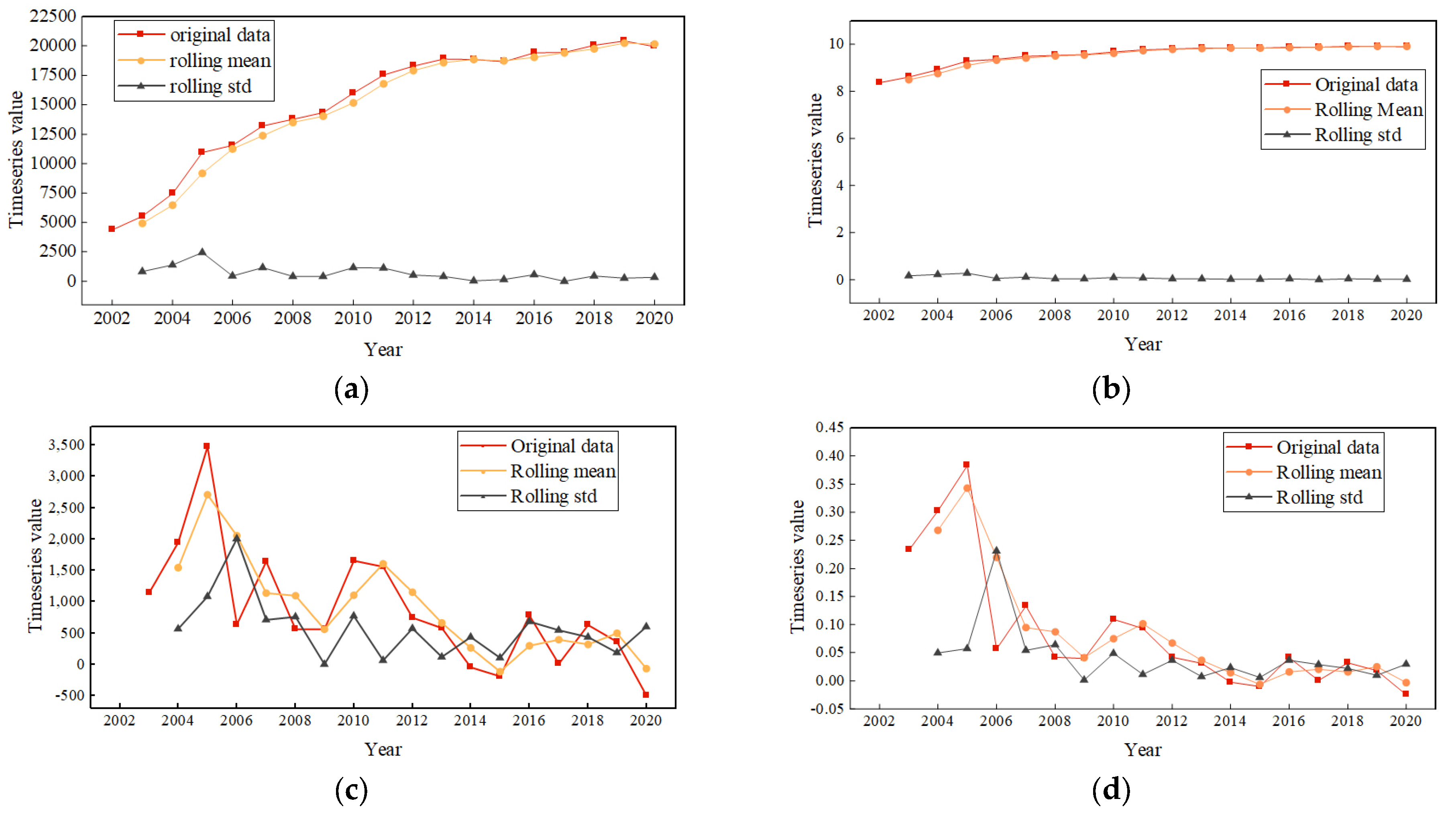
For time series drawing, perform a unit root test (such as the Dicky–Fuller test). The specific values should compare between the augmented Dickey–Fuller (ADF) statistic and the critical value. If the ADF statistic is less than the critical value at the corresponding significance level (usually 0.05), the data can be considered stable. For non-stationary sequences, first, perform differencing, or take the logarithm and then perform differencing. The d-value should be determined based on the difference order and converted into a stationary time series.

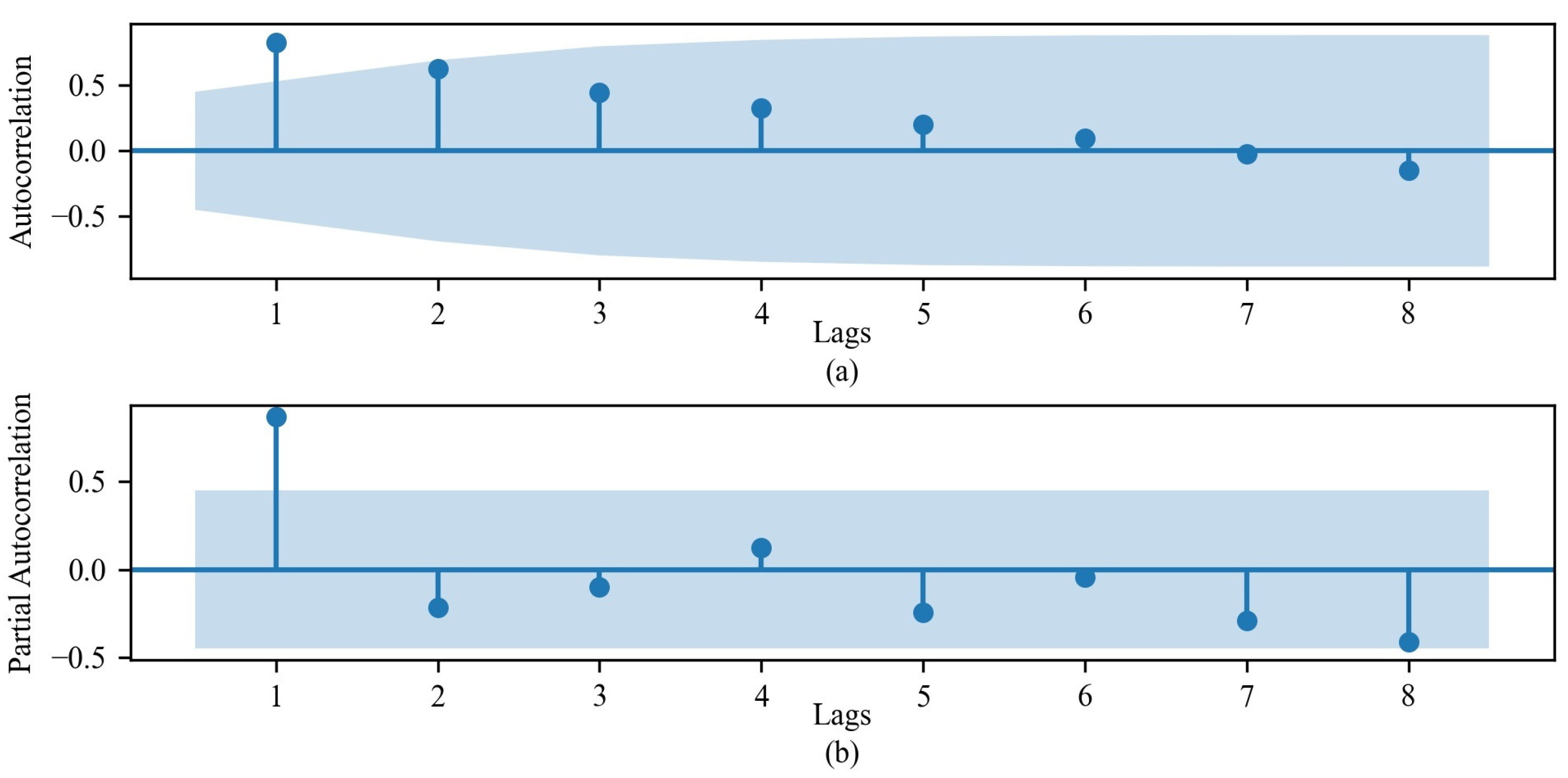
(2)

An autocorrelation coefficient and partial autocorrelation coefficient are obtained for the stationary time series, and the optimal order for p and q is estimated by analyzing the autocorrelation function (ACF) and partial autocorrelation (PACF), combined with the Akaike information criterion (AIC).

(3)

Based on the p, d, and q values obtained above, construct and fit the ARIMA models.

(4)

Check the residual of the model; the residual of a well-fitted model should be white noise. White noise means that the model captures most of the information in the data. For example, using the Ljung–Box test, if the p-value is greater than the significance level (0.05), the mean of the residuals is close to zero, the standard deviation is relatively stable, and the residuals are considered white noise. Successful modeling can be used for subsequent predictions.

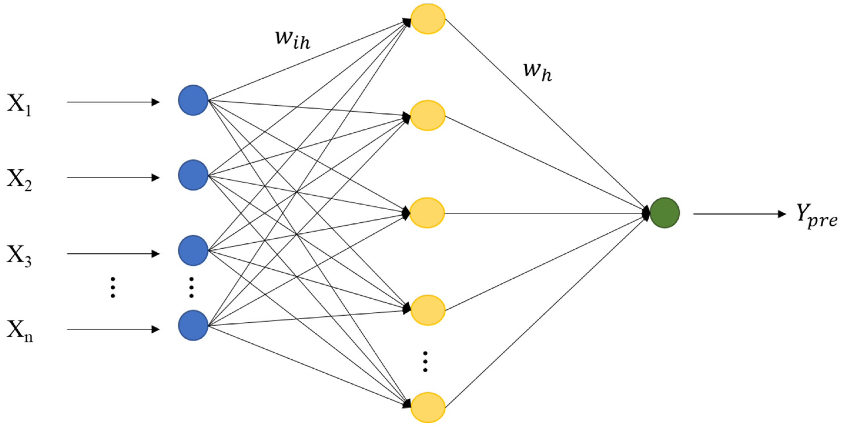
2.3. BPNN

The BPNN model is based on the error back-propagation algorithm and consists of an input layer, an output layer, and one or more hidden layers to form a multi-layer feed-forward neural network [31]. Each layer of neurons is connected to adjacent layers of neurons, allowing information to propagate forward and errors to propagate backward. The core idea of the BPNN algorithm is that the input layer first receives each neuron sample, calculates it layer by layer until the predicted value $Y_{pre}$ is generated in the output layer, calculates the error between the output layer $Y_{pre}$ and the true value, and then the error is reverse-propagated to the neurons of the neural network. Adjust the weights and biases within the neurons according to the direction of the error gradient descent to reduce errors. The training samples are calculated and adjusted in the adjusted neural network, and the cycle iteration is repeated until the error is below the threshold or enough iterations are reached that the iterations are stopped. The structure of the BPNN is shown in Figure 1.

In the figure, ${\omega }_{ih}$(i = 1, 2, …, n; h = 1, 2, …, m) are the connection weights between the input layer and the hidden layer; ${\omega }_h$ is the connection weight between the hidden layer and the output layer; n is the number of neurons in the input layer.

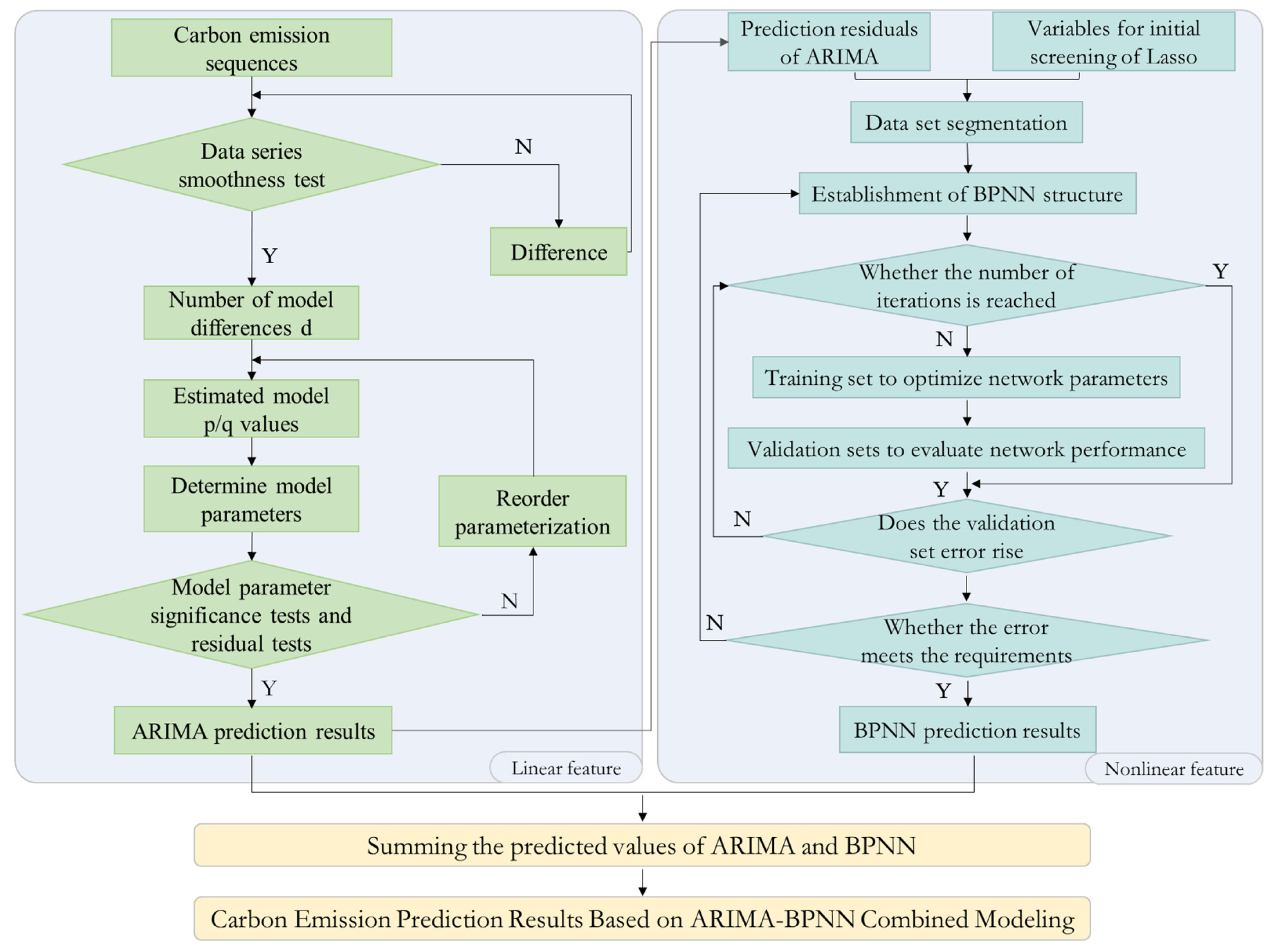
2.4. The Combination Model

The factors that affect carbon emissions include both linear and nonlinear factors, and using only an ARIMA or BPNN model may lead to significant errors. The ARIMA model is simple and easy to use, mainly suitable for linear relationships, but has limited ability in handling nonlinear and complex data. A BPNN can flexibly capture nonlinear relationships in data, which makes it mature and widely used. However, it is prone to fall into local optimal solutions and is sensitive to parameters such as the initial weights and learning rates. In large-scale networks and deep networks, the training time may be longer. For ARIMA models, coupling them with a BPNN model can compensate for the shortcomings of the ARIMA models related to nonlinear relationships. For BPNN models, although BPNNs may be able to achieve the desired accuracy on their own in some cases, the ARIMA models can preprocess the data before the BPNN and extract basic trend information, thus reducing the complexity of the model and making the neural network more focused on capturing nonlinear patterns. The calculation process is simplified by incorporating linear factors into the ARIMA model, which has a fast calculation speed and high accuracy, and compensates for the slow convergence speed of traditional neural networks, improving the overall generalization ability and robustness of the model.

In order to overcome the limitations of a single model, the ARIMA model and the BPNN are combined to give full play to the ARIMA model in fitting linear sequences and to the strong nonlinear mapping ability of the BPNN and thus improve the final prediction accuracy. As shown in Figure 2, the ARIMA model is first used to predict the carbon emissions, with the influencing factors obtained from the initial screening of the Lasso regression as the input variables for the BPNN model. The BPNN is used to predict the residual sequence of the ARIMA model, and the outputs of the two models are added as the final results on the carbon emissions, which can more accurately predict future carbon emissions.

3. Data and Empirical Research

3.1. Sources of the Data

The carbon emissions generated by energy consumption in the industrial sector, the electric power sector, the transportation sector, and the residential sector above a designated size in Suzhou from 2002 to 2020 represent the overall carbon emissions generated in Suzhou for the subsequent estimation. The electric power sector is generally classified as industrial in principle; with a relatively large amount of carbon emissions, its accounting is a bit different from that for other types of energy. Therefore, independent accounting is required for the power sector. The construction sector is also an important sector for carbon emissions. However, due to the fact that the carbon emissions generated by the construction sector mainly come from building material production and the transportation of and construction with building materials, the energy consumption of building material production is covered in the industrial sector, building material transportation is covered in the transportation sector, and building operation power consumption is included in the power sector accounting. The carbon emissions generated by construction are relatively small and almost negligible [32]. To avoid duplicate calculations, this study will no longer calculate the carbon emissions generated by the construction sector. The energy consumption data are sourced from the statistical yearbook of Suzhou City. The carbon emission factors of various energy sources mainly refer to the “Guidelines for the Compilation of Provincial Greenhouse Gas Inventories”. Some default values refer to the “2006 IPCC Guidelines for National Greenhouse Gas Inventory” (hereinafter referred to as the 2006 IPCC), and the carbon emission factors for electricity refer to the “Enterprise Greenhouse Gas Emission Accounting Methods and Reporting Guidelines for Power Generation Facilities (2022 Revised Edition)”. Based on the carbon emission factors for various energy sources, the carbon emissions of each department are calculated. The historical carbon emissions are shown in Figure 3. The carbon emission accounting for energy consumption is shown in Equation (3):

$$E={{\displaystyle \sum }}_{i}A{C}_i\times E{F}_i$$

(3)

where $A{C}_i$ is the activity level of i energy sources, and $E{F}_i$ is the emission factor for i energy sources.

3.2. The Lasso Regression Model

3.2.1. Lasso Regression Variable Selection

The factors that affect carbon emissions can be divided into population factors, economic factors, technological factors, and energy factors [33]. Based on previous research, 10 influencing factors are selected, including population size, urbanization rate, regional gross domestic product (GDP), regional per capita GDP, energy structure, industrial structure, energy consumption, overall social electricity consumption, energy consumption per unit of GDP, and carbon emission intensity. The main influencing factors are shown in

Table 1. Main influencing factors for carbon emissions.

Variable Type	Variables	Unit	Meaning of Indicators
Population factors	Population size	10,000	Total permanent resident population
	Urbanization rate	%	Urban population/permanent resident population
Economic factors	Regional gross domestic product (GDP)	Hundred million yuan	GDP
	Regional per capita GDP	10,000 yuan/person	Per capita GDP
Technical factors	Industrial structure	%	Value added of the secondary industry/GDP
Energy factors	Energy structure	%	Coal consumption/total energy consumption
	Energy consumption per unit of GDP	Tons of standard coal/10,000 yuan	Total energy consumption/GDP
	Total energy consumption	10,000 tons of standard coal	Total energy consumption
	Carbon emission intensity	Ton of carbon/10,000 yuan	Carbon dioxide emission/GDP
	Total electricity consumption	Ten thousand kilowatt-hours	Total electricity consumption

, and the data are sourced from the statistical yearbook of Suzhou.

The Lasso model was used to screen the key factors affecting carbon emissions from the 10 variables shown in Table 1, and the dependent variable was the annual carbon emissions in Suzhou City. Before selecting the variables, the data need to be standardized to eliminate the influence of dimensions. Considering the availability of predictive data and the degree of interpretation of influencing factors for carbon emissions, when the regularization parameter λ in the Lasso model takes a value of 0.0049 and the goodness of fit R² of the model is 0.998, 4 variables can be removed, which means that the 6 variables selected by the model can explain 99.8% of the changes in carbon emissions.

Table 2. Coefficients of various variables after compression.

Variables	Standardized Coefficient	R2
Total energy consumption	0.864	0.998
Carbon emission intensity	0.239
Total social electricity consumption	0.116
Total population	0.032
Energy structure	0.024
Energy consumption per unit of GDP	−0.207

shows the impact factors of the remaining 6 variables after compression.

3.2.2. Sensitivity Analysis of the Influencing Factors

As can be seen from Table 2, the degree of influence of the variables on carbon emissions is as follows: total energy consumption > carbon emission intensity > energy consumption per unit of GDP > total social electricity consumption > total population > energy structure. Among them, total energy consumption, carbon emission intensity, total social electricity consumption, permanent population, and energy structure have positive impacts on carbon emissions. When the other variables remain unchanged, with the total energy consumption increased by 1%, the carbon emissions increase by 0.864%. For an increase of 1% in the carbon emission intensity, carbon emissions increase by 0.239%. With an increase of 1% in electricity consumption in the whole population, carbon emissions increase by 0.116%. Meanwhile, an increase of 1% in the permanent population leads to a 0.032% increase in carbon emissions, and when the coal consumption share increases by 1%, carbon emissions increase by 0.024%. The standardization coefficient of energy consumption per unit of GDP is negative, indicating a negative correlation between energy consumption per unit of GDP and carbon emissions. This is different from most previous studies [34]. Although a decrease in energy consumption per unit of GDP indicates high energy utilization efficiency, it does not necessarily mean that carbon emissions will decrease, as the amount of carbon emissions also depends on factors such as total energy consumption [35], carbon emission intensity [4], and energy structure [36]. Due to Suzhou’s energy structure being mainly composed of high-carbon energy, with a large total energy consumption and a high carbon emission intensity, even if the energy consumption per unit of GDP is reduced, carbon emissions may still increase. From the historical data of Suzhou City from 2002 to 2020, it can be seen that the energy consumption per unit of GDP has decreased year by year, while the overall carbon emissions have increased year by year.

3.3. ARIMA Models

3.3.1. Determination of the ARIMA Model Parameters

The trend in carbon emissions with the rolling mean and variance in Suzhou from 2002 to 2020 is shown in Figure 4a. The carbon emissions show an upward trend over time, which belongs to a non-stationary sequence. In order to make the sequence stable, the logarithm of carbon emissions is first taken as shown in Figure 4b, and then the original sequence and the logarithmic sequence are differentiated separately, as shown in Figure 4c,d. Then, the unit root test is conducted, as shown in

Table 3. Unit root test results of carbon emissions.

Variable	p-Values	ADF Value	1% 1	5%	10%	Inspection Results
X	0.356201	−1.849451	−4.223238	−3.189369	−2.729839	Unstable
log(X)	0.760290	−0.980555	−4.223238	−3.189369	−2.729839	Unstable
Δlog(X)	0.000001	−5.634789	−4.223238	−3.189369	−2.729839	Stable

¹ 1%: A 1% level corresponds to a 99% confidence level, meaning there is only a 1% chance of incorrectly rejecting the null hypothesis (which states that the series has a unit root, implying non-stability). A 5% level corresponds to a 95% confidence level, and a 10% level corresponds to a 90% confidence level.

. After taking the natural logarithm of the carbon emission sequence and differencing it once, the p-value was 0.000001, which was less than the significance level (0.05), and the ADF test value was −5.634789, which was less than the critical value at the 99%, 95%, and 90% confidence levels, so they were judged to be relatively stable using the unit root test. Compared with Figure 4c,d, after one differencing, the data became more stable, and the rolling mean and rolling standard deviation of the data were also more stable. Therefore, first-order differencing was chosen, which is the parameter (d = 1) of the ARIMA model.

The values of p and q can be estimated by observing the ACF plot and the PACF plot of a stationary sequence as shown in Figure 5a,b, respectively. The ACF plot shows the correlation between the time series and different lag values, while the PACF shows the partial correlation between the time series and its lag values. As shown in the figure, the ACF plot is trailing after the first order, so q is 1. The PACF plot is truncated after the first order, so p is 1. However, based on the image, the values of p and q have a certain degree of subjectivity. After multiple experiments, the AIC was used to determine the optimal combination of the ARIMA model parameters. As the goal of the AIC is to find a balance between good fitting and model complexity, the smaller the AIC value is, the better the model is considered. When the model is ARIMA (1, 1, 1), the AIC value of the model is −30.39, which is relatively small. Then, Ljung–Box testing was used to test whether the residual was white noise. The results are shown in

Table 4. White noise test values for residuals.

p-Values
1	2	3	4	5	6	7	8
0.712339	0.789016	0.911048	0.116968	0.193629	0.286803	0.390002	0.412298

, and the p-values are all greater than the significance level (0.05), indicating it is white noise. The ARIMA (1, 1, 1) model is suitable and can effectively extract information.

3.3.2. ARIMA Model Prediction

Given that the ARIMA model has been effectively validated for predicting future carbon emissions in the previous part, the training and validation sets will no longer be divided here. Instead, data from Suzhou City 2002–2020 will be directly used as the samples to fit the ARIMA model. The prediction results are shown in Figure 6a. It is seen that the ARIMA model’s accuracy in predicting carbon emissions is not satisfactory, but the trend is consistent, indicating that the model grasps the information on the linear part of carbon emissions.

3.4. The BPNN

The six influencing factors selected using the Lasso regression model are used as inputs for the BPNN, and carbon emissions are used as the outputs. Considering the limited sample data, the mean of all the input and output data is standardized before modeling. The sample data from 2002 to 2017 are used as the training set, while the sample data from 2018 to 2020 are used as the validation set. The number of neurons in the input layer is set to 6, and the number of neurons in the output layer is set to 1. Since there is no authoritative method to determine the number of hidden layers and neurons, they are normally set based on multiple training and testing. After multiple training and testing stages, the hidden layer is set to 1, with 3 neurons. The activation function of the hidden layer is the tanh function, and the activation functions of the input and output layers are sigmoid and linear functions, respectively. The number of network learning epochs is set to 500 with a learning rate of 0.01. Upon completion of the 500-epoch training, the loss function reaches stability, and the model converges, requiring a total of 29.34 s. The root mean square error (MSE) of the loss function is calculated based on Equation (4). The fitting effect of the model after multiple training stages is shown in Figure 6b.

$$MSE=\frac{1}{n}{{\displaystyle \sum }}_{i=1}^n{\left(y_i-\widehat{y_i}\right)}^2$$

(4)

In the equation, n represents the number of samples; $y_i$ represents the i-th true value; i represents the index of the sample, i = 1, 2, …, n; $\widehat{y_i}$ represents the predicted value of the i-th true value.

3.5. ARIMA-BPNN

Firstly, the ARIMA (1, 1, 1) model is used to predict the carbon emission sequence y_t from 2002 to 2020. The original data sequence is Y. The residual sequence e of the ARIMA (1, 1, 1) model is e = Y − y_t, which serves as the output variable of the ARIMA-BPNN combination model. The residual sequence predicted using the combination model is e_t, and the final prediction sequence Y_t is the sum of the two, i.e., Y_t = e_t + y_t. The six variables selected using the Lasso model are used as inputs for the ARIMA-BPNN model. In the combination model, the number of neurons in the input layer of the BPNN is 6, the number of neurons in the output layer is 1, and the number of neurons in the hidden layer is 3. The sample data from 2002 to 2017 are used as the training set, and the sample data from 2018 to 2020 are used as the validation set. After preprocessing and multiple training and testing stages, the network parameters are determined to be linear functions for the activation functions of each layer, the number of learning epochs is 300, the learning rate is 0.01, and the MSE is used for the loss function. Upon the completion of 300 training epochs, the loss function stabilizes, taking 8.94 s. This represents a 69.53% improvement in the training speed compared to a standalone BPNN. The prediction results of the combination model are shown in Figure 6c.

3.6. Model Result Analysis

In previous studies, the percentage mean absolute error (MAE_P), mean absolute percentage error (MAPE), percentage root mean square error (RMSE_P), and goodness of fit R² have mainly been selected as the evaluation indexes for a model’s prediction accuracy. Besides the above indexes, this work also selects the absolute percentage error (APE) and residuals to measure the difference between the annual true value and the model’s predicted value to better evaluate the predictive performance of the model. The calculation formulas are shown in Equations (5) and (6). MAE_P represents the average magnitude of the model’s prediction error, which is not sensitive to outliers. The calculation formula is shown in Equation (7). MAPE is the average relative error between the true value and the predicted value, expressed as a percentage, as shown in Equation (8). When considering errors, RMSE_P gives a higher weight to larger errors and is more sensitive to larger values of prediction errors, as shown in Equation (9). R² represents the degree of explanation of the model for the dependent variable, ranging from 0 to 1. The closer the value is to 1, the better the model fits the true value, as shown in Equation (10). The smaller the MAE_P, MAPE, and RMSE_P values are, the better the performance of the model.

$$APE=\left|\frac{y_i-\widehat{y_i}}{y_i}\right|$$

(5)

$$\mathrm{Residuals}=y_i-\widehat{y_i}$$

(6)

$$MA{E}_P=\frac{\frac{1}{n}{{\displaystyle \sum }}_{i=1}^n\left|y_i-\widehat{y_i}\right|}{\overline{y}}$$

(7)

$$MAPE=\frac{1}{n}{{\displaystyle \sum }}_{i=1}^n\left(\frac{\left|y_i-\widehat{y_i}\right|}{y_i}\right)$$

(8)

$$RMS{E}_P=\frac{\sqrt{\frac{1}{n}{{\displaystyle \sum }}_{i=1}^n{\left(y_i-\widehat{y_i}\right)}^2}}{y_{max}-y_{min}}$$

(9)

$$R^2=1-\frac{{{\displaystyle \sum }}_{i=1}^n{\left(y_i-\widehat{y_i}\right)}^2}{{{\displaystyle \sum }}_{i=1}^n{\left(y_i-\overline{y}\right)}^2}$$

(10)

where n represents the number of samples; $y_i$ represents the i-th true value; i represents the index of the sample, i = 1, 2, …, n; $\widehat{y_i}$ represents the predicted value of the i-th true value; $\overline{y}$ represents the average value of true value, i.e., $\overline{y}=\frac{1}{n}{{\displaystyle \sum }}_{i=1}^n{y}_i$.

It can be seen from Figure 7 and Figure 8 that the error of the BPNN fitting results is the largest. Compared with the single model, the error of the ARIMA-BPNN combined model is reduced. As depicted in Figure 7, the APE of the ARIMA model ranges from a minimum of 0.003580 to a maximum of 0.99, with a mean of 0.115. The APE of the BPNN model ranges from a minimum of 0.00080 to a maximum of 1.15, with a mean of 0.123. The APE of the combined ARIMA-BPNN model ranges from a minimum of 0.000758 to a maximum of 0.62, with a mean of 0.081. All these indicators of the combined model are smaller than the single model. Additionally, the standard deviations of the APE of the ARIMA model, the BPNN, and the ARIMA-BPNN combination model were calculated to be 0.23, 0.30, and 0.14, respectively, indicating that the stability of the ARIMA-BPNN model surpasses that of the single model.

Table 5. Performance comparison between the single model and combined model.

Evaluating Index	ARIMA	BPNN	ARIMA-BPNN
MAEP	6.55%	5.66%	5.23%
MAPE	11.49%	12.32%	8.09%
RMSEP	9.02%	9.80%	6.88%
R2	91.56%	89.36%	95.09%

shows the prediction performance of the single model and the combined model. The MAE, MAPE, and RMSE of the ARIMA-BPNN combined model are 5.23%, 8.09%, and 6.88%, respectively, which are the lowest values of the three groups of models, 20.15%, 29.59%, and 23.72% lower than that of ARIMA model and 7.60%, 29.59%, and 23.72% lower than that of the BPNN. The combined model had the highest R² of 95.09%, which is 3.86% and 6.41% higher than that of the single ARIMA model and the BPNN, respectively, showing higher prediction accuracy and model robustness. From the above, it is noted that the ARIMA-BPNN combination model has higher prediction accuracy and can effectively predict carbon emissions. Given the variability in the prediction regions and data samples, fluctuations in the evaluation metrics are expected [21]. As shown in

Table 6. Results of different studies.

Model	R2	Reference
GA-BP	0.853	Peng, et al. [37]
SPNN-GNWR	0.89	Tang [38]
ARIMA-BP	0.951

, the ARIMA-BPNN combined model demonstrates a significant improvement in R², indicating a superior predictive accuracy over the study by Peng et al. [37], as well as by Tang [38].

4. Scenario Setting and Analysis of the Prediction Results

4.1. Scenario Descriptions

Based on the background of “carbon neutrality, carbon peak”, this study integrates the dual-carbon policy measures enacted by the national and Suzhou municipal governments, taking into account the main factors affecting carbon emissions. Three scenarios are established based on the rate of change in the influencing factors, the timing of peak emissions, and the quantity of emissions at peak: the baseline scenario, the low-carbon scenario, and the demonstration scenario.

Benchmark scenario: The benchmark scenario set in this article refers to the social and economic development status and future carbon emission trends of Suzhou City under the constraints of the existing policy measures. Due to the current introduction of relevant policies, such as the “Outline of the 14th Five-Year Plan and Long-term Goals of Suzhou City” (hereinafter referred to as the “The 14th Five-Year Plan”) and the Population Development Plan, in order to achieve these policy goals, the development of various influencing factors may no longer follow the historical trends but will undergo new changes. This scenario analyzes the future carbon emission trends of Suzhou City under the existing planning.

Low-carbon scenario: This scenario refers to the adoption of more proactive policy measures by Suzhou City on the basis of the benchmark scenario, accelerating energy structure adjustment; promoting low-carbon transformation in sectors such as industry, electricity, transportation, and construction; improving energy efficiency and clean energy utilization; reducing carbon emission intensity; and achieving the carbon peak and carbon neutrality goals by 2060.

Demonstration scenario: This scenario is based on a low-carbon scenario, where Suzhou City further increases its emission reduction efforts; fully leverages the demonstration and leading role of a strong industrial city; accelerates the promotion of advanced modes such as green manufacturing, intelligent manufacturing, and circular manufacturing; and not only achieves carbon peaking ahead of schedule but also achieves carbon neutrality ahead of schedule.

4.2. Parameter Settings

The core of the scenario analysis is to determine the influencing factors and parameters. Six indicators selected using Lasso regression are used as the main influencing factors for scenario analysis. Taking 2020 as the benchmark year, the total energy consumption (Supplementary Material File S1), carbon emission intensity (File S1), permanent population (File S1), energy structure (File S1), energy consumption per unit GDP (File S1), and total social electricity consumption (Supplementary Material File S2) of Suzhou City from 2021 to 2060 are predicted according to the relevant policies. A long-term forecast of the carbon emissions in Suzhou City from 2021 to 2060 is conducted. The prediction of each parameter in the three scenarios is shown in Supplementary Material Files S1 and S2.

4.3. Analysis of the Prediction Results

Based on the three scenario paths set above, the ARIMA-BPNN combination model is used to predict the carbon emissions of Suzhou City from 2021 to 2060. The CO₂ trends in Suzhou under different scenarios are shown in Figure 9. The analysis of the carbon emissions in Suzhou under various scenarios is as follows.

Benchmark scenario: Under the constraints of the existing policy planning, the economy maintains rapid development, and fossil fuels such as coal remain the main energy source. Suzhou’s CO₂ emissions cannot peak in 2030 but will peak five years later in 2035, an increase of 52.26 million tons compared to 2020, reaching 251.60 million tons. After reaching their peak, carbon emissions slowly decrease. By 2060, carbon emissions will decrease by 82.49 million tons compared to 2035, 52.26 million tons compared to 2020, and to 169.11 million tons.

Low-carbon scenario: Compared to the benchmark scenario, under the low-carbon scenario, economic development slows down, the proportion of clean energy increases rapidly, the electrification process accelerates, and Suzhou’s CO₂ emissions peak in 2030. The carbon emissions are 222.48 million tons, an increase of 23.14 million tons compared to 2020 and a decrease of 29.12 million tons compared to the peak of the baseline scenario in 2030. Subsequently, carbon emissions slowly decrease between 2025 and 2035, and after 2035, the rate of decline accelerates. By 2060, carbon emissions reach 105.90 million tons. Compared to 2020, they decrease by 903.44 million tons, and compared to the baseline scenario, the annual carbon emissions for carbon neutrality decrease by 63.21 million tons.

Demonstration scenario: Compared to the benchmark scenario, the demonstration scenario aims to achieve early peaking and carbon neutrality. In this scenario, the CO₂ emissions in Suzhou City reach their peak 5 years earlier, reaching 208.29 million tons in 2025, an increase of 8.95 million tons compared to 2020, and a decrease of 43.31 million tons and 14.19 million tons, respectively, compared to the peaks of the benchmark and low-carbon scenarios. Subsequently, carbon emissions rapidly decrease, reaching only 53.39 million tons by 2060, a decrease of 145.95 million tons compared to 2020 and a decrease of 115.72 million tons and 52.51 million tons, respectively, compared to the neutrality year in the benchmark and demonstration scenarios.

5. Conclusions and Policy Proposals

5.1. Conclusions

A Lasso-ARIMA-BPNN combination model is built to predict the medium-and long-term carbon emission trends in Suzhou City. Based on the Lasso regression model, the main factors affecting carbon emissions in Suzhou City are screened, and three scenario models are set up using scenario analysis methods to provide policy recommendations and inspiration for low-carbon development in Suzhou City. The main conclusions are as follows.

(1)

The variables obtained from the initial screening of the Lasso model are able to explain 99.8% of the carbon emissions in Suzhou, indicating that the variables obtained from the compression of the Lasso model are the main influencing factors for carbon emissions. The number of variables used in constructing the model is relatively small, simplifying the complexity of carbon emission analysis and prediction and improving the efficiency and accuracy of the model.

(2)

Based on the variable screening using the Lasso model, the six main factors affecting carbon emissions in Suzhou City are the total energy consumption, carbon emission intensity, total social electricity consumption, total population, energy structure, and energy consumption per unit of GDP. The impact of the total social electricity consumption on carbon emissions cannot be ignored.

(3)

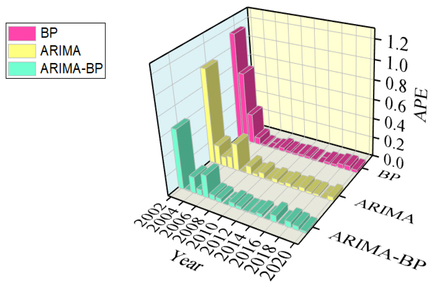
Based on the historical data of Suzhou City from 2002 to 2020, the single (ARIMA, BPNN) model and the ARIMA-BPNN combination models were established, respectively. Based on the fitting results, the ARIMA-BPNN combination model has a higher prediction accuracy. The linear fitting characteristics of the ARIMA model and the nonlinear mapping ability of the BPNN model are effectively utilized to improve the prediction ability for carbon emissions.

(4)

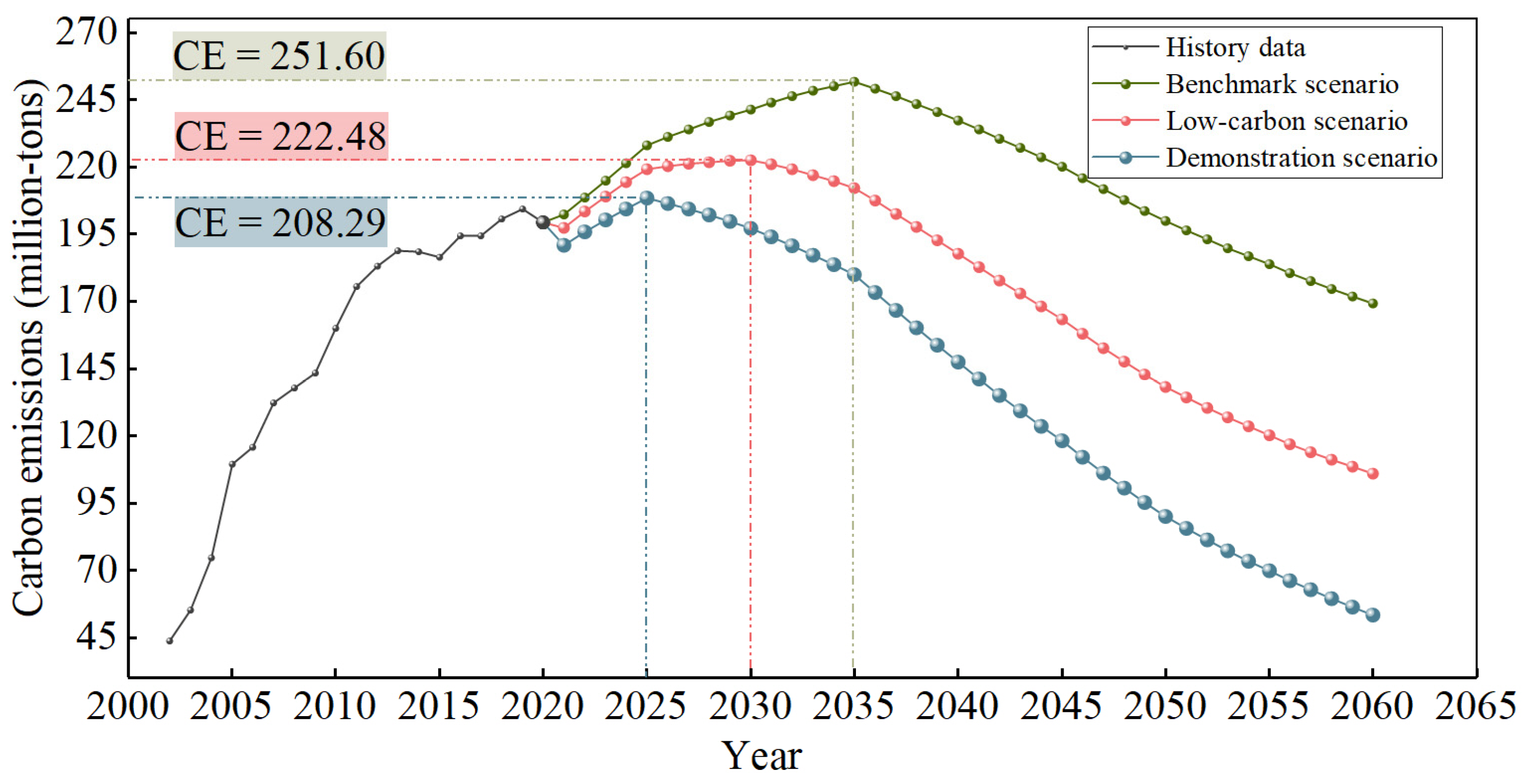
Under the constraints of the existing policy measures, Suzhou cannot achieve its carbon peak as scheduled. By adjusting the speed of economic development and the energy consumption structure, Suzhou City can achieve a carbon peak before 2030. This suggests that there is still significant room for optimization in the industrial and energy structures of Suzhou City.

5.2. Policy Proposal

Based on empirical analysis, suggestions are proposed for Suzhou City to achieve its carbon peak and carbon neutrality targets as scheduled for reference.

(1)

Speeding up the adjustment of the energy consumption structure. Based on the results of the Lasso regression analysis, total energy consumption, carbon emission intensity, and energy structure all have a positive impact on CO₂ emissions, with total energy consumption being the primary factor affecting carbon emissions. In Suzhou, the high proportion of high-energy-consuming industries, where coal consumption is the main energy source and the main source of carbon emissions, leads to a high carbon emission intensity. In this context, in order to control carbon emissions and achieve carbon peaking and carbon neutrality as scheduled, it is necessary for the government to increase its policy efforts on carbon reduction, control the total energy consumption, reduce the use of coal and other high-carbon fossil fuels, increase the proportion of non-fossil energy consumption, accelerate the elimination of an outdated production capacity, and promote green and low-carbon development in key industries.

(2)

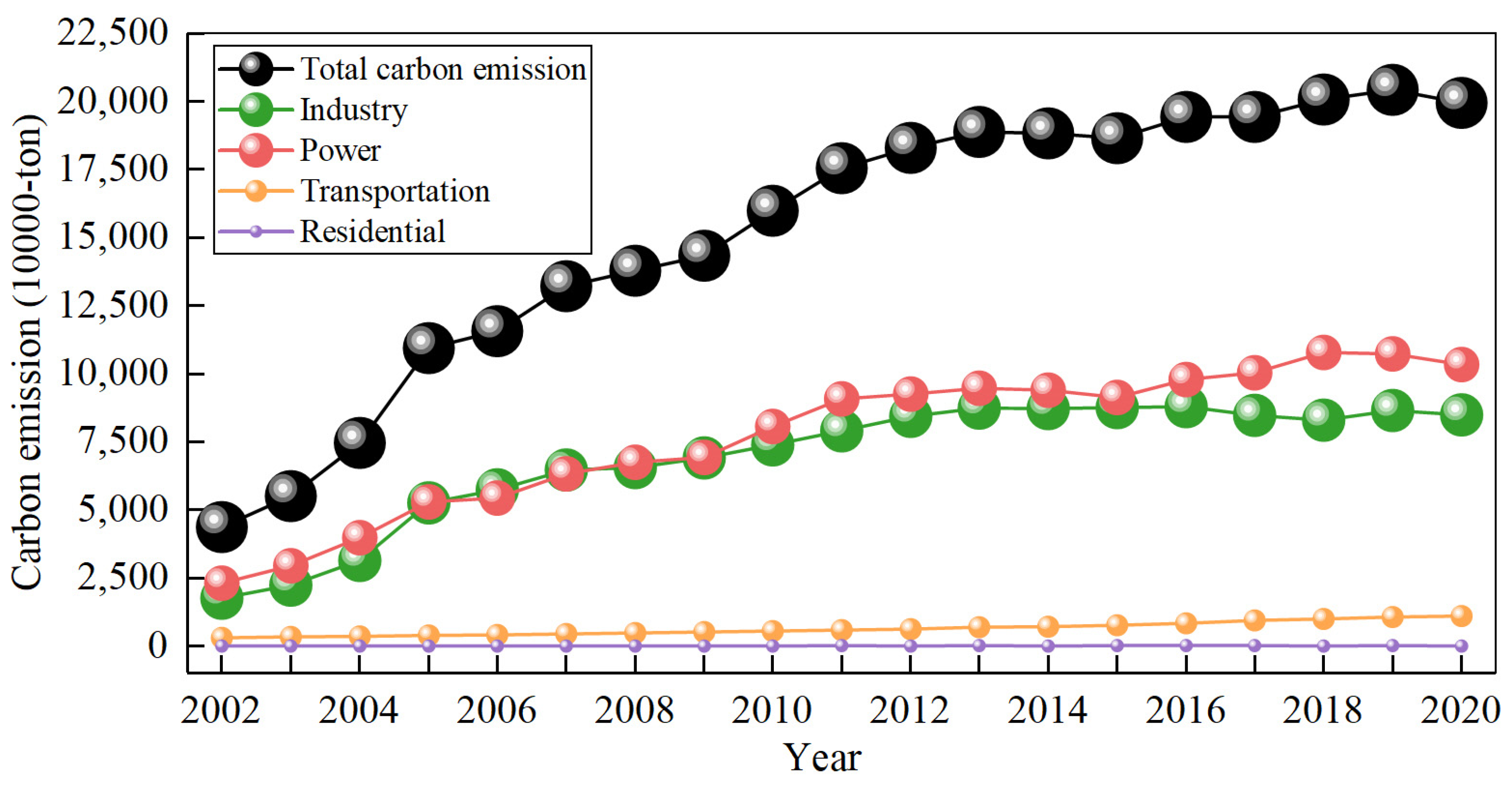
Promoting the cleanliness of electricity. The results of the Lasso regression indicate that the total electricity consumption has a significant positive impact on the increase in carbon emissions in Suzhou, with a standardized coefficient of 0.116. From 2002 to 2020, the total electricity consumption in Suzhou has seen an upward trend. As shown in Figure 3, the power sector is another major source of carbon emissions in Suzhou apart from the industrial sector. Therefore, it is necessary to promote the clean-up of electricity. The whole city should focus on the power supply side, with photovoltaic and wind power as the main sources, supplemented by biomass power generation. The situation of comprehensive electrification on the demand side, supplemented by hydrogen energy and coal as a guarantee, should be developed. Electrification does not emit carbon dioxide on the consumption side. The substitution of electricity for coal and oil should be vigorously promoted. The government should promote the development of clean electricity, improve the electrification level of the terminal electricity departments, and reduce carbon emissions.

6. Challenges and Prospects

Although certain wonderful results are achieved in carbon emission prediction, there are still shortcomings and challenges that need to be further improved and perfected in subsequent research.

(1)

The data used in this article come from statistical yearbooks and the relevant literature, which may have certain inaccuracies and incompleteness, affecting the predictive performance of the model. Attempt to use more data sources, such as satellite remote sensing data, social media data, etc., in future research may be able to improve the quality and coverage of the data.

(2)

Although the scenario analysis method used in this work can simulate different carbon emission paths, there is still a certain degree of uncertainty and subjectivity, such as the range of influencing factors, the setting and assumptions of scenarios, etc. Further research can attempt to use various scenario analysis methods, such as Monte Carlo simulation, system dynamics simulation, etc., to improve the reliability and scientificity of the scenario analysis.

(3)

The policy proposals in this paper may provide some references for the low-carbon development of Suzhou City, while limitations and difficulties still exist, such as the feasibility, coordination, and execution of the policies. An attempt to adopt policy evaluation methods, such as cost–benefit analysis, multi-criteria decision analysis, etc., would be able to improve the effectiveness and relevance of the policy recommendations.

References

1. Li, Q.; Sheng, B.; Huang, J.; Li, C.; Song, Z.; Chao, L.; Sun, W.; Yang, Y.; Jiao, B.; Guo, Z.; et al. Different climate response persistence causes warming trend unevenness at continental scales. Nat. Clim. Chang. 2022, 12, 343–349. [Google Scholar] [CrossRef]
2. Masson Delmotte, V.; Zhai, P.; Pirani, A.S.; Connors, L.; Péan, C.; Chen, Y.; Goldfarb, L.; Gomis, M.I.; Robin Matthews, J.B.R.M.; Berger, S.; et al. Climate Change 2021: The Physical Science Basis of Working Group I Contribution to the Sixth Assessment Report of the Intergovernmental Panel on Climate Change; Cambridge University Press: Cambridge, UK; New York, NY, USA, 2021. [Google Scholar] [CrossRef]
3. Wang, H.; Lu, X.; Deng, Y.; Sun, Y.; Nielsen, C.P.; Liu, Y.; Zhu, G.; Bu, M.; Bi, J.; McElroy, M.B. China’s CO2 peak before 2030 implied from characteristics and growth of cities. Nat. Sustain. 2019, 2, 748–754. [Google Scholar] [CrossRef]
4. Li, S.; Siu, Y.W.; Zhao, G. Driving Factors of CO2 Emissions: Further Study Based on Machine Learning. Front. Environ. Sci. 2021, 9, 721517. [Google Scholar] [CrossRef]
5. Zhang, P.L.; Du, Q.J. On Influencing Factors of Carbon Emissions in Beijing-Tianjin-Hebei Region: Based on the Extended STIRPAT Model. Sci. Technol. Manag. Land Resour. 2022, 39, 14–23. [Google Scholar] [CrossRef]
6. Ren, F.; Long, D. Carbon emission forecasting and scenario analysis in Guangdong Province based on optimized Fast Learning Network. J. Clean. Prod. 2021, 317, 128408. [Google Scholar] [CrossRef]
7. Neves Pedreira, V.; Lapa Brito, M.; Lobato dos Santos, L.C.; George, S. Modeling of Brazilian Carbon Dioxide Emissions: A Review. Braz. Arch. Biol. Technol. 2022, 65, e22210594. [Google Scholar] [CrossRef]
8. Chen, C.; Liu, C.; Wang, H.; Jing, G.; Chen, L.; Wang, H.; Zhang, J.; Li, Z.; Liu, X. Examining the impact factors of energy consumption related carbon footprints using the STIRPAT model and PLS model in Beijing. China Environ. Sci. 2014, 34, 1622–1632. [Google Scholar]
9. Mitchell, L.E.; Lin, J.C.; Bowling, D.R.; Pataki, D.E.; Strong, C.; Schauer, A.J.; Bares, R.; Bush, S.E.; Stephens, B.B.; Mendoza, D.; et al. Long-term urban carbon dioxide observations reveal spatial and temporal dynamics related to urban characteristics and growth. Proc. Natl. Acad. Sci. USA 2018, 115, 2912–2917. [Google Scholar] [CrossRef] [PubMed]
10. Wu, S.; Zhang, K. Influence of Urbanization and Foreign Direct Investment on Carbon Emission Efficiency: Evidence from Urban Clusters in the Yangtze River Economic Belt. Sustainability 2021, 13, 2722. [Google Scholar] [CrossRef]
11. Dong, F.; Li, X.-h. The influencing factors analysis of Chinese carbon emissions based on the co-integration analysis with the help of grey correlation analysis (GRA). In Proceedings of the 2011 IEEE International Conference on Grey Systems and Intelligent Services, Nanjing, China, 15–18 September 2011; pp. 149–153. [Google Scholar] [CrossRef]
12. Tsai, C.; Chang, C.; Chen, L. Applying Grey Relational Analysis to the Vendor Evaluation Model. Int. J. Comput. Internet Manag. 2003, 11, 45–53. [Google Scholar]
13. Qi, Y.; Liu, H.; Zhao, J.; Xia, X. Prediction model and demonstration of regional agricultural carbon emissions based on PCA-GS-KNN: A case study of Zhejiang province, China. Environ. Res. Commun. 2023, 5, 051001. [Google Scholar] [CrossRef]
14. Van Der Cam, A.; Adant, I.; Van den Broeck, G. The social acceptability of a personal carbon allowance: A discrete choice experiment in Belgium. Clim. Policy 2023, 23, 859–871. [Google Scholar] [CrossRef]
15. Liu, S.; Chen, H.; Liu, P.; Qin, F.; Fars, A. A novel electricity load forecasting based on probabilistic least absolute shrinkage and selection operator-Quantile regression neural network. Int. J. Hydrogen Energy 2023, 48, 34486–34500. [Google Scholar] [CrossRef]
16. Liu, H.; Liu, Y.; Wang, C.; Song, Y.; Jiang, W.; Li, C.; Zhang, S.; Hong, B. Natural Gas Demand Forecasting Model Based on LASSO and Polynomial Models and Its Application: A Case Study of China. Energies 2023, 16, 4268. [Google Scholar] [CrossRef]
17. Song, J.; Zhang, Y. Scene Prediction of China‘s Carbon Emissions Based on BP Neural Network. Sci. Technol. Eng. 2011, 11, 4108–4111. [Google Scholar] [CrossRef]
18. Wen, L.; Liu, Y. A research about Beijing’s carbon emissions based on the IPSO-BP model. Environ. Prog. Sustain. Energy 2017, 36, 428–434. [Google Scholar] [CrossRef]
19. Ren, F.; Guo, M. Research on net carbon emissions, influencing factor analysis, and model construction based on a neural network model in the BTH region. J. Renew. Sustain. Energy 2022, 14, 066101. [Google Scholar] [CrossRef]
20. Chen, R.; Ye, M.; Li, Z.; Ma, Z.; Yang, D.; Li, S. Empirical assessment of carbon emissions in Guangdong Province within the framework of carbon peaking and carbon neutrality: A lasso-TPE-BP neural network approach. Environ. Sci. Pollut. Res. 2023, 30, 121647–121665. [Google Scholar] [CrossRef]
21. Wen, T.; Liu, Y.; Bai, Y.H.; Liu, H. Modeling and forecasting CO2 emissions in China and its regions using a novel ARIMA-LSTM model. Heliyon 2023, 9, e21241. [Google Scholar] [CrossRef]
22. Sun, Y.; Yang, Y.; Liu, S.; Li, Q. Research on Transportation Carbon Emission Peak Prediction and Judgment System in China. Sustainability 2023, 15, 14880. [Google Scholar] [CrossRef]
23. Egeh, O.M.; Chesneau, C.; Muse, A.H. Exploring hybrid models for forecasting CO2 emissions in drought-prone Somalia: A comparative analysis. Earth Sci. Inform. 2023, 16, 3895–3912. [Google Scholar] [CrossRef]
24. Cheng, W.; Zhou, Y.; Guo, Y.; Hui, Z.; Cheng, W. Research on prediction method based on ARIMA-BP combination model. In Proceedings of the 2019 3rd International Conference on Electronic Information Technology and Computer Engineering (EITCE), Xiamen, China, 18–20 October 2019; pp. 663–666. [Google Scholar] [CrossRef]
25. Yan, W.; Xiao, J.; Ding, G. Application of ARIMA model and BP neural network model in prediction of tuberculosis incidence in Gansu Province. Chin. J. Dis. Control Prev. 2019, 23, 729–732. [Google Scholar] [CrossRef]
26. Dou, Z.; Ji, M.; Wang, M.; Shao, Y. Price Prediction of Pu’er tea based on ARIMA and BP Models. Neural Comput. Appl. 2022, 34, 3495–3511. [Google Scholar] [CrossRef] [PubMed]
27. Zhao, C.; Mao, C. Forecast of Intensity of Carbon Emission to China Based on BP Neural Network and ARIMA Combined Model. Resour. Environ. Yangtze Basin 2012, 21, 665–671. [Google Scholar]
28. Li, J.; Zhang, X. Beijing-Tianjin-Hebei Energy Demand Combination Forecast Analysis. IOP Conf. Ser. Earth Environ. Sci. 2021, 631, 012104. [Google Scholar] [CrossRef]
29. Tibshirani, R. Regression Shrinkage and Selection Via the Lasso. J. R. Stat. Soc. Ser. B (Methodol.) 1996, 58, 267–288. [Google Scholar] [CrossRef]
30. Box, G.E.P.; Jenkins, G.M.; Reinsel, G.C. Time series analysis forecasting and control. J. Time 2010, 31, 238–242. [Google Scholar] [CrossRef]
31. Rumelhart, D.E.; Hinton, G.E.; Williams, R.J. Learning representations by back-propagating errors. Nature 1986, 323, 533–536. [Google Scholar] [CrossRef]
32. Cai, W.; Wu, Y.; Ni, H.; Yu, Y.; Wu, J.; Fu, Y.; Wang, B.; Shao, Q.; Fu, Y.; Hu, S.; et al. 2022 Research Report of China Building Energy Consumption and Carbon Emissions; China Association of Building Energy Efficiency: Beijing, China, 2022; Available online: http://www.199it.com/archives/1568439.html (accessed on 14 September 2023).
33. Yang, P.; Liang, X.; Drohan, P.J. Using Kaya and LMDI models to analyze carbon emissions from the energy consumption in China. Environ. Sci. Pollut. Res. 2020, 27, 26495–26501. [Google Scholar] [CrossRef]
34. Naminse, E.Y.; Zhuang, J. Economic Growth, Energy Intensity, and Carbon Dioxide Emissions in China. Pol. J. Environ. Stud. 2018, 27, 2193–2201. [Google Scholar] [CrossRef]
35. Osobajo, O.A.; Otitoju, A.; Otitoju, M.A.; Oke, A. The Impact of Energy Consumption and Economic Growth on Carbon Dioxide Emissions. Sustainability 2020, 12, 7965. [Google Scholar] [CrossRef]
36. Yin, T. The diversity of energy consumption structure, energy efficiency and carbon emissions: Evidence from Shaanxi, China. PLoS ONE 2023, 18, e0285738. [Google Scholar] [CrossRef] [PubMed]
37. Peng, S.; Tan, J.; Ma, H. Carbon emission prediction of construction industry in Sichuan Province based on the GA-BP model. Environ. Sci. Pollut. Res. 2024, 31, 24567–24583. [Google Scholar] [CrossRef] [PubMed]
38. Tang, H. Research on Carbon Emission Prediction Based on Spnn and Gnnwr Models—Take the Yangtze River Delta as an Example. Master’s Thesis, Nanjing University of Posts and Telecommunications, Nanjing, China, 2022. [Google Scholar]
39. Liu, W.; Chen, Y. Economic development between the “two centuries”: Tasks, challenges and response strategies. Social Sciences in China 2021, 3, 86–102. [Google Scholar]
40. Wei, Y.; Yu, B.; Tang, B.; Liu, L.; Liao, H.; Chen, J.; Sun, F.; Runying, A.; Wu, Y.; Tan, J.; et al. Roadmap for Achieving China’s Carbon Peak and Carbon Neutrality Pathway. J. Beijing Inst. Technol. (Soc. Sci. Ed.) 2022, 24, 13–26. [Google Scholar] [CrossRef]
41. He, J.; Li, Z.; Zhang, X.; Wang, C.; Wang, H.; Wang, X.; Tian, Z.; Bai, Q.; Cong, J.; Du, E. China’s Long-term Low-carbon Development Strategies and Pathways Comprehensive Report. China Popul. Resour. Environ. 2020, 30, 1–25. [Google Scholar] [CrossRef]
42. Li, H.; Mao, X.; Zhu, L.; Yao, Y.; Tan, J. Saturation Load Forecasting Based on Long Short-Time Memory Network. In Proceedings of the 2018 2nd IEEE Conference on Energy Internet and Energy System Integration (EI2), Beijing, China, 20–22 October 2018; pp. 1–6. [Google Scholar] [CrossRef]
43. Zhai, X.; Tian, S.; An, Q.; Chen, W.; Li, J. Automatic Coordinated Control Technology of Incremental Distribution Network Based on Saturated Load Forecasting. Tech. Autom. Appl. 2022, 41, 123–127. [Google Scholar]
44. Tian, S.; Zhou, Q.; Cheng, H.; Liu, L.; Lu, L.; Jiang, S. Application of pigeon-inspired optimization algorithm based SVM in total power demand forecasting. Electr. Power Autom. Equip. 2020, 40, 173–181. [Google Scholar] [CrossRef]
45. Qin, H.; Luo, C.; Bao, Z.; Huang, L.; Li, K.; Chen, L. Medium-long term electricity consumption prediction considering future scenario constraints. Power Demand Side Manag. 2022, 24, 59–66. [Google Scholar] [CrossRef]
Figure 1. Three-layer BPNN structure diagram.
Energies 17 01856 g001
Figure 2. ARIMA-BPNN combination model flowchart.
Energies 17 01856 g002
Figure 3. Carbon emission trends in various departments in Suzhou City.
Energies 17 01856 g003
Figure 4. Data and their rolling mean and variance. (a) For original data; (b) for logarithm; (c) for original data after first difference; (d) for logarithmic data after first difference.
Energies 17 01856 g004
Figure 5. Autocorrelation and partial autocorrelation graphs of time series. (a) ACF plot; (b) PACF plot.
Energies 17 01856 g005
Figure 6. Fitting of the models. (a) ARIMA; (b) BPNN; (c) ARIMA-BPNN combination.
Energies 17 01856 g006
Figure 7. APE values fitted using three models.
Energies 17 01856 g007
Figure 8. Error bands for fitting three models.
Energies 17 01856 g008
Figure 9. Carbon emission prediction results under three scenarios.
Energies 17 01856 g009