Abstract
This paper presents a current control design for stabilizing an inductive-capacitive-inductive (LCL)-filtered grid-connected inverter (GCI) system under uncertain grid impedance and distorted grid environment. To deal with the negative impact of grid impedance, LC-type grid impedance is considered in both the system model derivation and controller design process of an LCL-filtered GCI system. In addition, the integral and resonant control terms are also augmented into the system model in the synchronous reference frame to guarantee the reference tracking of zero steady-state error and good harmonic disturbance compensation of the grid-injected currents from GCI. By considering the effect of grid impedance on the control design process, an incomplete state feedback controller will be designed based on the linear-quadratic regulator (LQR) without damaging the asymptotic stabilization and robustness of the GCI system under uncertain grid impedance. By means of the closed-loop pole map evaluation, the asymptotic stability, robustness, and resonance-damping capability of the proposed current control scheme are confirmed even when all the system states are not available. In order to reduce the number of required sensors for the realization of the controller, a discrete-time current-type full-state observer is employed in this paper to estimate the system state variables with high precision. The feasibility and effectiveness of the proposed control scheme are demonstrated by the PSIM simulations and experiments by using a three-phase GCI prototype system under adverse grid conditions. The comprehensive evaluation results show that the designed control scheme maintains the stability and robustness of the LCL-filtered GCI when connecting to unexpected grids, such as harmonic distortion and L-type and LC-type grid impedances. As a result, the proposed control scheme successfully stabilizes the entire GCI system with high-quality grid-injected currents even when the GCI faces severe grid distortions and an extra grid dynamic caused by the L-type or LC-type grid impedance. Furthermore, low-order distortion harmonics come from the background grid voltages and are maintained as acceptable limits according to the IEEE Std. 1547-2003. Comparative test result with the conventional one also confirms the effectiveness of the proposed control scheme under LC-type grid impedance thanks to the consideration of LC grid impedance in the design process.
1. Introduction
The growing global energy demand results in the energy transition, which increases the percentage of renewable energy sources (RESs) in the total energy generation. Solar and wind energy sources are mostly used around the globe thanks to their accessibility, affordability, and the fast development of power electronics to effectively integrate RES power into the utility grid [1]. Recently, the grid-connected inverter (GCI) has played the main role not only in injecting renewable energy into the main grid but also in improving the power quality in case there are several serious disturbances in the main grid environment [2].
Generally, to maximize the power conversion efficiency in the control of the GCI system, a pulse width modulation (PWM) scheme is deployed with a high switching frequency. Additionally, to meet the standard of power quality, such as the IEEE Std. 1547 [3], high switching frequency harmonics in the GCI output currents should be attenuated effectively by filters. For this aim, the inverter is connected to the main utility grid through a low pass filter such as L or LCL type filter. In comparison to the L-type filter, the higher order filter, like the LCL type, is preferred thanks to its excellent harmonic attenuation capability with smaller physical size and weight [4,5,6]. However, the LCL filter introduces the resonance phenomenon in the inverter operation, which should be mitigated by damping techniques [7].
Damping techniques to suppress the resonance caused by LCL filters can be commonly classified as passive and active damping techniques. The passive damping methods are implemented by attaching a physical resistor to the filter capacitor branch to reduce the resonance peak. Even though this method is simple and effective, it results in additional loss of power via passive resistance [8]. On the other hand, the active damping technique presented in [9] uses a virtual resistance concept to alleviate the resonance phenomenon without any extra power loss due to physical resistance. However, this active damping technique has the problem of increasing the complexity of the overall system configuration by requiring an extra number of sensors. As another active damping technique, a full-state feedback control scheme can compensate for the resonance caused by the LCL filter straightforwardly and flexibly [10,11]. Since this control scheme needs the information of all system states for the realization of the damping, full-state observers are commonly adopted to decrease the number of sensing devices in real operation.
Apart from the attenuation of the high switching frequency components, low order frequency components at orders of 5th, 7th, 11th, and 13th in the distorted grid voltages due to the non-ideal grid should also be considered in the design process of the current controller. Generally, the proportional-resonant (PR) controllers constructed in several forms are widely used to compensate for such distortions in the grid-side currents [12,13]. The study in [14] presented the full-state feedback current controller designed in the synchronous reference frame (SRF). In this study, the integral control and resonant control terms are augmented into the system model in the state space to obtain the control objectives of the reference tracking and grid voltage distortion attenuation. Another method to deploy the PR control was presented in [15], in which the PR control is represented in the form of the discrete-time transfer function. However, it is worth mentioning that those studies are not robust against the system uncertainty introduced by filter component variations or unexpected grid impedance.
Another challenge in the GCI system design is the additional impedance linking between the GCI and the main grid [16]. Since RES can be installed from various geographical regions, the renewable power is normally transferred to the main grid and loaded via a long transmission line, which forms an inevitable grid impedance. It is well known in numerous studies that the negative effects of grid impedance increase the complexity of RES system dynamics and raise a challenge to maintain the stability of the integration system and the power quality. Furthermore, the grid impedance variation also severely affects the performance of both the active damping and harmonic compensation [17].
In general, there are two types of grid impedance: L-type and LC-type. L-type impedance is caused by the long transmission line, which makes the point of the common coupling (PCC) become weak and influences the stability of the GCI system. The weak grid problem has been widely studied in [18,19], in which several current controllers have been presented to ensure the robustness of inverter operation against the L-type grid impedance variation. Particularly, the study in [18] presents an impedance-phased compensation control method to enhance the stability of GCIs with L-type grid impedance variation. However, the scheme in [18] requires prior knowledge of the grid inductance information. A control scheme for an LCL-filtered inverter under a non-ideal grid, such as a weak grid, is proposed by taking into consideration the parameter uncertainties [20]. The research work in [21] investigates the stability margins of the conventional current control methods under a weak grid.
The study in [22] presents a linear matrix inequality (LMI)-based model predictive current control for LCL-filtered GCIs under unexpected grid and system uncertainties. Impedance-based stability analysis is also investigated for a single-phase inverter [23]. However, the above control schemes cannot guarantee system stability under LC-type grid impedance. To further extend the robustness of parallel-connected GCIs against the weak, distorted grid conditions, a robust control scheme is presented in [24], which effectively attenuates the distortion harmonics in the main grid up to the 21st order.
Besides the impact of the inductance component in the main grid, the grid impedance may contain both inductive and capacitive components, which form the complex grid condition [25,26,27]. Recently, since more and more power electronic devices are integrated into the power grid, the grid condition has become more complex. The main grid contains not only an unknown inductance component caused by a long transmission line but also a capacitive component formed by the power factor correction, which harms the stability of the LCL-filtered GCI system. As compared to the studies regarding L-type impedance, only a few studies considering the LC-type impedance in the current control design process of GCI systems have not been conducted. In [25,26,27], the control schemes are designed based on the passivity-based stability criterion to enhance the stability of a GCI system under various grid conditions. In [25], the interconnection stability of the L-filter inverter connected with a complex grid has been fully assessed via the dissipative properties of inverter input admittance, in which the accuracy of the input-admittance model is improved by taking the PWM and sampling processes into consideration. Other research work in [26] investigates the passivity of the GCI system equipped with LCL filters, in which both converter-side current feedback control and grid-side current feedback control structures are evaluated to study the system stability regions when connecting to the complex grid. However, the grid background harmonics are not considered in this study. An inverter output impedance enhancing control mechanism realized by an additional hardware setup has been presented in [27] to guarantee sufficient passivity to grid disturbances. The robustness of the presented method against several grid conditions is guaranteed at the expense of an additional complex hardware setup.
From a different point of view, additional LC-type grid impedance can be considered as an extra LC-filter stage linked to the LCL-filtered inverter. A current control scheme should also be designed to drive the inverter system stably with an LCL filter connected to an extra LC filter stage caused by the complex grid. Even under LC-type grid impedance, all the system state variables introduced by the LCL-filtered GCI can be obtained by constructing a state observer, as mentioned in [19]. In addition, the PCC voltages serve as additional states for the capacitance of the LC-type grid impedance. However, the current flowing through the grid inductance cannot be measured. As a result, a full-state feedback current controller cannot be realized because of the absence of a state for grid inductance current when the grid has the LC-type grid impedance.
Inspired by the idea to design a controller by using the linear quadratic regulator (LQR) with incomplete state feedback for a tracking problem in [28], an LQR-based state feedback current controller is developed for an LCL-filtered GCI under the circumstance of the complex grid in this paper. When the grid has the LC-type grid impedance, the current flowing through the grid impedance is not possible to be measured or estimated. In this case, it is not possible to implement a full-state feedback control because the grid inductance current is not available. To overcome such a limitation, an incomplete state feedback control approach is implemented by removing the unmeasured state feedback control term for the state of the grid inductance current. Other control objectives of harmonic disturbance compensation and zero steady-state tracking error are achieved by augmenting the multiple internal control terms in the inverter system model.
To systematically obtain the gain set in the proposed current controller, the optimal gain is first derived from the standard LQR problem. For this purpose, the model of the LCL-filtered GCI with LC-type grid impedance is derived with the values of grid inductance and grid capacitance set to certain values. Then, the integral and resonant control terms are augmented into the system model, and the feedback control gain is derived from the standard LQR problem. Finally, the gain matrix to achieve the incomplete state feedback current control is derived from the optimal gain matrix by simply eliminating the columns corresponding to the state variables of grid inductance currents. By means of the closed-loop pole map evaluation, the asymptotic stability, robustness, and resonance-damping capability of the proposed current control scheme based on the incomplete state feedback are confirmed. The feasibility and effectiveness of the proposed current control scheme are demonstrated by the Powersim (PSIM) software (version 9.1) simulations and experiments by using a three-phase GCI prototype system under adverse grid conditions such as harmonic distortion, L-type, and LC-type grid impedances. The main contributions of this paper are summarized as follows:
- (i)
- To deal with the negative impact of grid impedance, LC-type grid impedance is considered in both the system model derivation and controller design process of an LCL-filtered GCI system. The proposed scheme ensures the reference tracking of zero steady-state error and good harmonic disturbance compensation of the grid-injected currents. By considering the effect of grid impedance on the control design process, an incomplete state feedback current controller is designed based on the LQR without damaging the asymptotic stabilization and robustness of the GCI system under uncertain grid impedance.
- (ii)
- By means of the closed-loop pole map evaluation, the asymptotic stability, robustness, and resonance-damping capability of the proposed control scheme are confirmed even when all the system states are not available. The proposed control scheme successfully stabilizes the entire GCI system with high-quality grid-injected currents even when the GCI faces severe grid distortions and an extra grid dynamic caused by the L-type or LC-type grid impedance.
- (iii)
- The comprehensive evaluation results show that the designed control scheme maintains the stability and robustness of the LCL-filtered GCI when connecting to unexpected grid such as the harmonic distortion, L-type and LC-type grid impedances. Comparative test result with the conventional one also confirms the effectiveness of the proposed control scheme.
2. System Model of a GCI with LC-Type Grid Impedance
2.1. Modeling of a GCI
To design the current controller and the state observer in the SRF, the phase variables in “abc” are transformed to DC variables in “dq” by the Park’s transformation as
where f represents the variables to be transformed and is the phase angle.
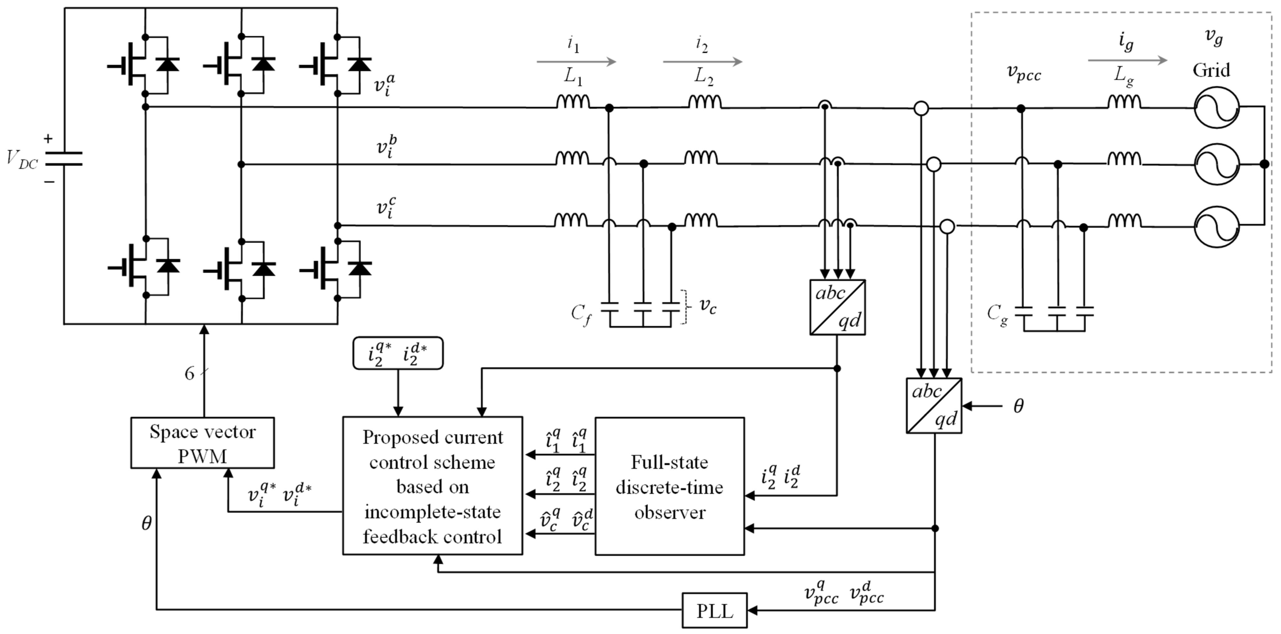
Figure 1 represents the configuration of an LCL-filtered GCI, which is connected to the grid with LC-type impedance, and the proposed scheme is based on incomplete state feedback control. In the proposed scheme, six states of the LCL-filtered GCI are estimated from the full-state observer. In Figure 1, i1, i2, and vc are the inverter-side current, the grid-side current, and the capacitor voltage, respectively, vpcc is the PCC voltage, vg is the utility grid voltage, VDC is the DC-link voltage, ig is the grid inductance current, and vi is the inverter output voltage. The PCC voltage vpcc is the same as the utility grid voltages vg if the grid impedance does not exist. The parameters and denote the filter inductances, denotes the filter capacitance, and and denote the inductance and capacitance caused by the LC-type grid impedance. The symbol ‘^’ denotes the estimated quantity, and ‘*’ denotes the reference quantity. The conventional phase lock loop (PLL) is employed to determine the phase angle of the grid voltage by using the PCC voltages at the SRF. The reference voltages generated by the proposed control scheme are applied by the space vector PWM.

Figure 1.
The proposed incomplete state feedback current control scheme.
The state equations of the LCL-filtered GCI system and LC-type grid impedance are expressed mathematically in the SRF as follows:
where the superscript “q” and “d” denote the q-axis and d-axis. Also, , are the inverter-side current, the grid-side current, and the grid inductance current; is the angular frequency of grid voltage.
Using (2)–(11), the inverter system is expressed in the continuous-time state-space as follows:
where is the system state vector, is the system input vector, is the grid voltage vector, and the system matrices A, B, C, and D are expressed as:
2.2. Discrete-Time System Model
The continuous-time state-space model in (12) and (13) can be discretized for a digital implementation as follows:
where , , , and are expressed as
where Ts is the sampling period.
When implementing the current controller for a GCI system in digital hardware, the controller output u(k) computed at the kth step time is modulated by the space vector PWM at the next sampling time to apply the reference voltages to the real system. In other words, the actual controller output applied to the system at the present time step is u(k − 1), which causes the one-step delay. The one-step delay is also included in the modeling of the system in (16) by considering u(k) as additional state variables of ud (k) as below [29]:
Equations (22) and (23) are combined to present the entire system model in the matrix form as below:
3. Proposed Control Scheme with Incomplete Observation under Grid Uncertainties
In this section, an incomplete state feedback current control scheme is designed to stabilize the LCL-filtered GCI under LC-type grid impedance. The control objectives of good harmonic compensation and reference tracking are realized by augmenting the multiple internal control components in the inverter system model in state space. To systematically obtain the gain set in the proposed current controller, the gain matrix is derived based on the standard LQR problem, considering the partial state feedback problem.
3.1. Current Controller Design Considering L-/LC-Type Grid Impedance
The integral and resonant control components are combined in the discrete-time inverter system model to achieve the reference tracking and harmonic compensation objectives, respectively. In continuous time, an integral control component is expressed as [30]:
where is the integral control state is the current error vector, is the current reference vector, , and .
To compensate for the harmonic distortion, resonant control components tuned at the orders of 6th and 12th in the SRF are designed as below [14,31]
where is the resonant control state, is the damping ratio, , and .
The state equations of the integral and resonant control components in (26) and (27) are combined as
where is the state variables for integral and resonant terms, is the state vector for the integral term, is the state vector for the resonant term in the order of 6th, is the state vector for the resonant term in the order of 12th
For the aim of digital implementation, the combined state equations for the integral and resonant terms in (28) can be discretized as
where and are expressed as
By combining (25) with (29), the entire system model for a GCI control under the existence of LC-type grid impedance can be represented as follows:
Or, Equation (32) is rewritten as
The entire system model consisting of 22 states in (32) has three terms, which are the inverter system model and LC-type grid impedance as expressed in (16), one-step delay of controller output in (23), and an integral-resonant controller embedded in the system in (29).
Generally, the full-state feedback control scheme can be successfully applied for stabilizing the system (32) when all system state variables are available, as expressed below:
where .
is a feedback gain, represents the component for state feedback control gain, represents the component for the delay step feedback control gain, and represents the component for the integral and resonant feedback control gain.
By the LQR approach, the optimal controller gain in (34) is attained by minimizing the cost function (35) as [32,33]
where is positive semi-definite matrix and is positive definite matrix. The optimal gain is obtained by selecting the weighting matrices and according to the relative importance of the state variables and expense of energy. In this study, the optimal controller gains are attained by the Matlab Control System Toolbox version 10.11 function “dlqr”.
By means of the optimal gain K, the closed-loop dynamic is expressed as
This system is asymptotically stable with the eigenvalues of closed-loop matrix maintained inside the unit circle.
However, the grid inductance current ig in (12) or (25) cannot be measured or estimated due to the fact that exact grid impedance information is rarely known in practice. Then, the available state variables are presented as follows:
where .
To overcome this limitation in this study, an LQR current controller based on the incomplete state feedback is presented. In the incomplete state feedback control, the number of available feedback states is less than the total number of system state variables. Particularly, in the case that the only available states given by (37) are fed back, the control output u(k) in (33) is generated in a different form as
In this case, the control output in (38) applied into the system (33) generates the closed-loop dynamic as
The gain matrix needs to be obtained to ensure the matrix in (39) is stable, or all eigenvalues lie inside the unit circle. Based on the study in [28], in this study, the gain set is obtained from the submatrix of gain as
As a result, the closed-loop dynamic system (33) is derived as
The incomplete state feedback control gain is presented as follows:
By using the incomplete state feedback control gain in (34), the control output is finally determined as
where represents the state feedback control that does not include the grid inductance current ig states. By means of the closed-loop pole map evaluation, the asymptotical stability of the incomplete state feedback control derived by the LQR concept in (38) will be confirmed in the next subsection.
3.2. LQR-Based Discrete-Time Observer
To implement the incomplete state feedback control, the state variables except for the grid inductance current ig should be available. For the aim of reducing the number of required sensors, a system model-based state observer is deployed to estimate the states of the LCL-filtered GCI system. Using (2)–(7), the LCL-filtered GCI model expressed as six state equations can be represented in the continuous-time as
where is the state, is the PCC voltage, and , , , and are obtained as
The inverter system in (44) and (45) is discretized as
where
There are several kinds of observer types such as the prediction observer, current observer, and reduced-order observer [29]. In this study, the full-state current-type observer is deployed in discrete time because of its superior performance in comparison with other observer types. From (48) and (49), the full-state current-type observer is constructed as [14,29]
where is the observer gain, is the estimated state from the system dynamics and input at . The eigenvalues of should be maintained within the unit circle to guarantee the stability of observer. By means of the LQR approach, the observer gains are selected by using the Matlab function “dlqr”.
3.3. Stability Analysis Considering Grid Impedance
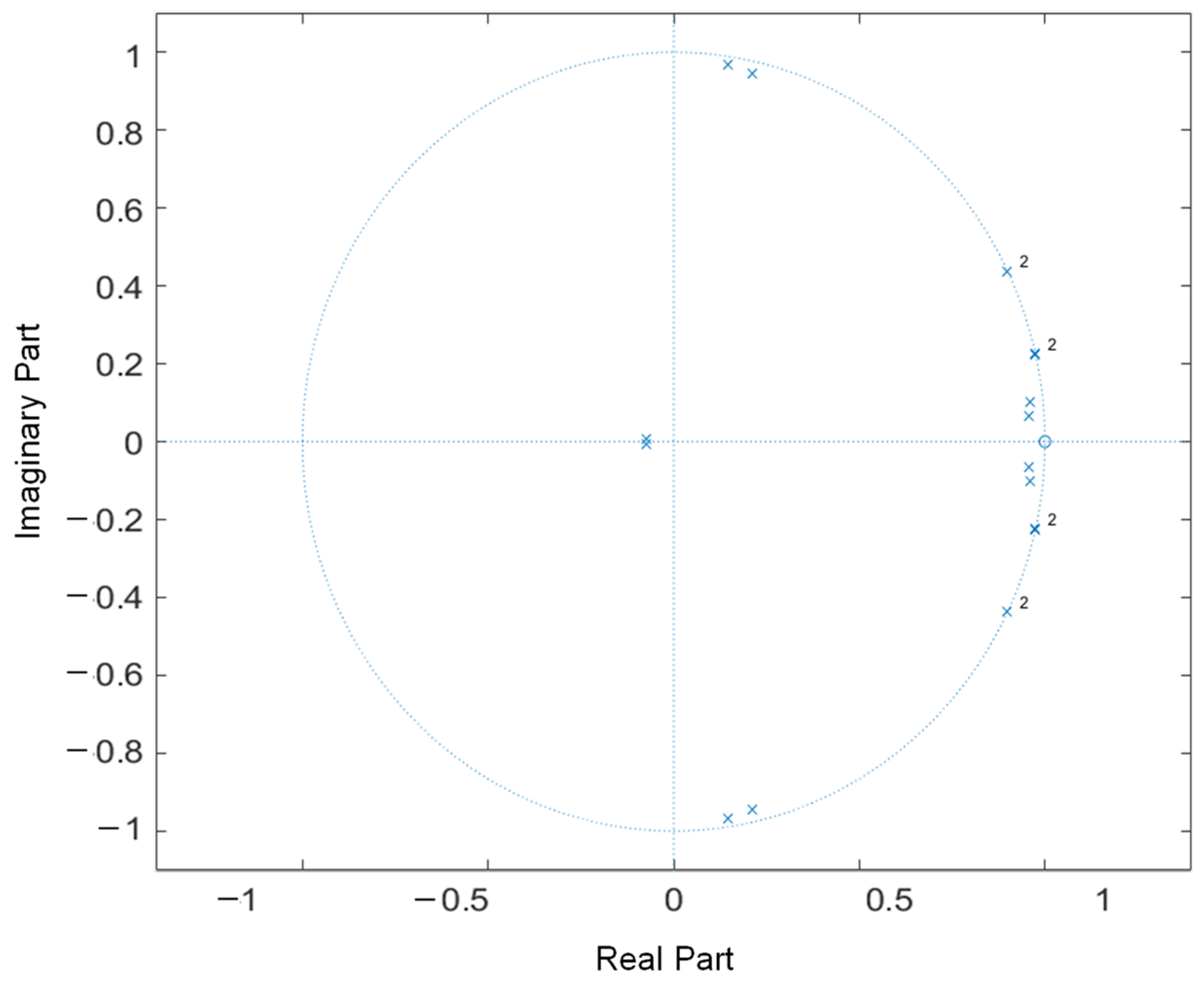
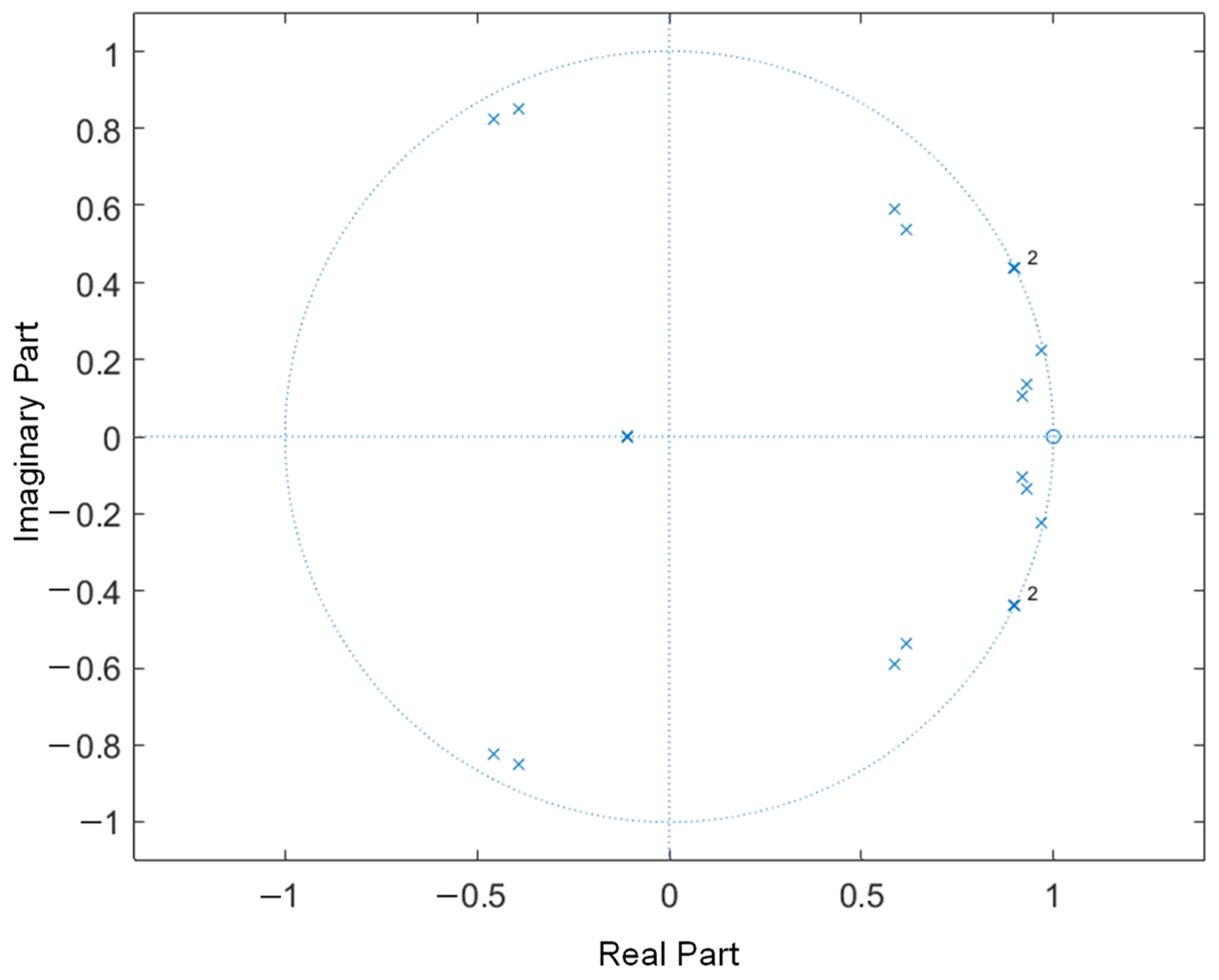
In this subsection, the closed-loop pole map of the LCL-filtered GCI system controlled by the proposed incomplete state feedback control is presented. To demonstrate the performance and robustness of the proposed scheme, all the eigenvalues of the matrix in (39) should lie inside the unit circle. Figure 2 represents the stability analyses when the grid impedance exists as an uncertain L-type with of 7 mH. Figure 3 represents the stability analyses for the complex grid setup, in which a grid inductance and a grid capacitance are selected as 3 mH and 10 µF, respectively. It is clear from Figure 2 and Figure 3 that even if the GCI system is faced with L-type or LC-type grid impedance, all eigenvalues are maintained inside the unit circle. These results effectively prove the stability of the LCL-filtered GCI controlled by the proposed incomplete feedback control scheme.
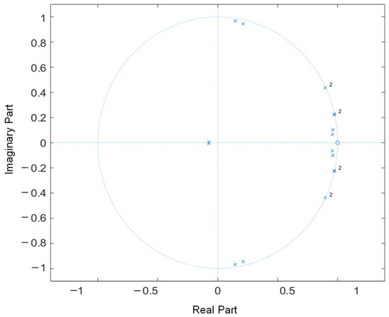
Figure 2.
Eigenvalues of the matrix when uncertain L-type grid impedance with of 7 mH exists.
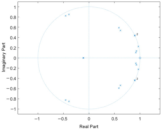
Figure 3.
Eigenvalues of the matrix when uncertain LC-type grid impedance (= 3 mH and = 10 µF) exists.
4. Simulation Results
In this section, the PSIM simulations have been conducted to verify the performance of the LCL-filtered GCI driven by the proposed current controller under stiff grid and uncertain grid impedances. The GCI system parameters and the grid impedance setup are shown in Table 1.

Table 1.
GCI System parameters and grid impedance setup.
4.1. Performance under Stiff Grid
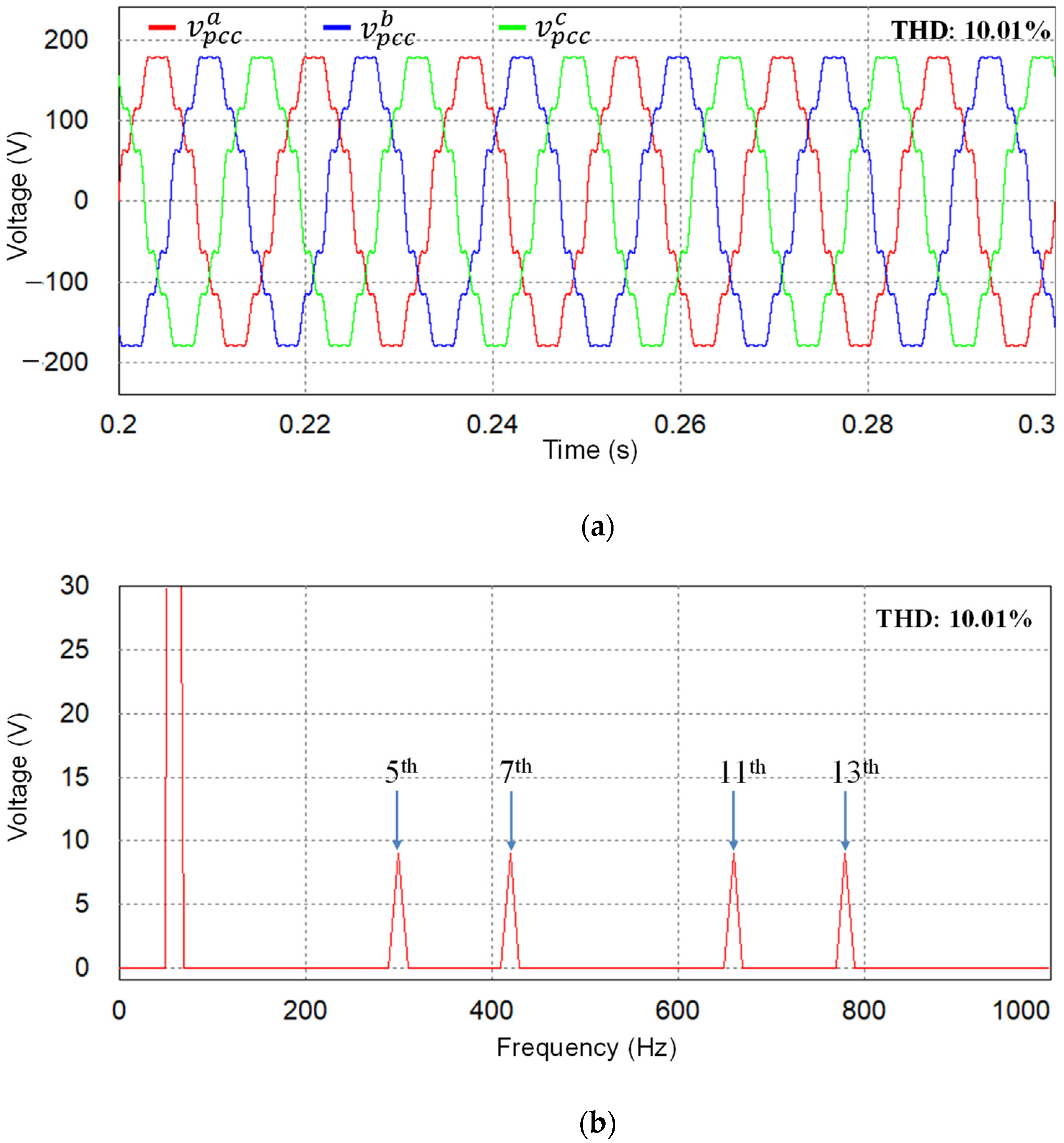
In the first test, the GCI is connected directly to the main grid without the existence of grid impedance. The three-phase distorted PCC voltages (same as the grid voltages in this case) are presented in Figure 4a with low-order distortion harmonics at the 5th, 7th, 11th, and 13th. The FFT analysis of a-phase PCC voltage in Figure 4b clearly highlights that the contaminated harmonic level of each component is set to 5% of the fundamental grid voltage magnitude, which produces the total harmonic distortion (THD) level of grid voltage to be 10.01%.
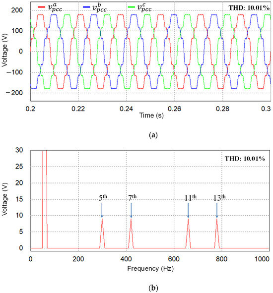
Figure 4.
Three-phase distorted PCC voltages under a stiff grid. (a) Distorted PCC voltages; (b) FFT result of a-phase PCC voltage.
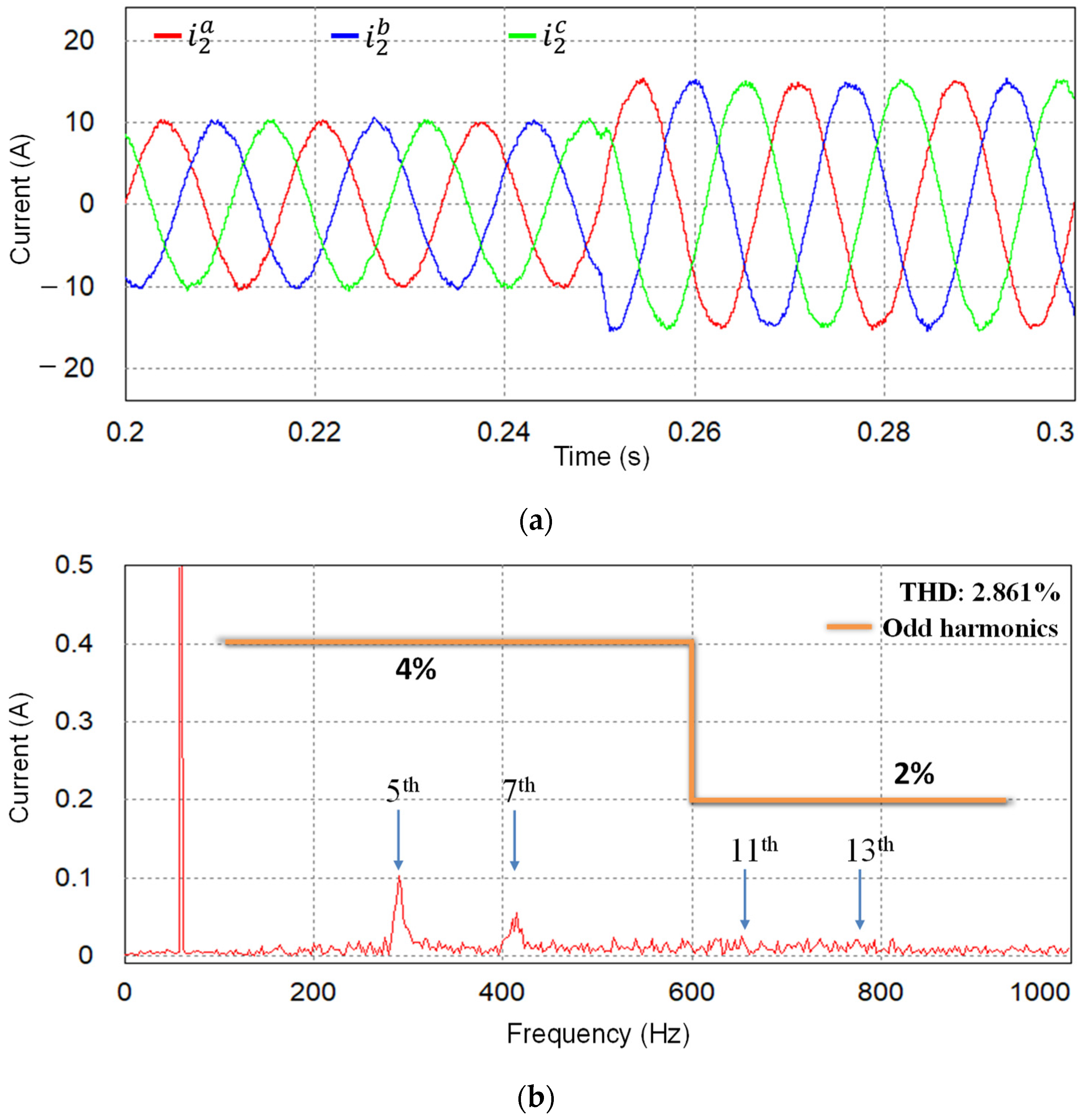
Under the stiff and distorted grid conditions, the grid-side current response of the proposed current controller is presented in Figure 5a. By means of the proposed controller, stable and high-quality grid-side currents can be produced in steady-state with a low THD level of 2.861%. The test result also demonstrates the effectiveness of active damping action realized by the state feedback controller and the harmonic compensation by resonant control terms augmented inside the controller. To verify the transient response, the grid-side current reference is changed from 10 A to 15 A at 0.25 s. The rapid reference tracking performance without any overshoot clearly shows a stable operation of the GCI controlled by the proposed control. The FFT result of grid a-phase current in Figure 5b also confirms that the individual harmonic distortion in grid-side current is maintained to be lower than the maximum limits specified in the IEEE Std. 1547-2003 [3] for a GCI system.
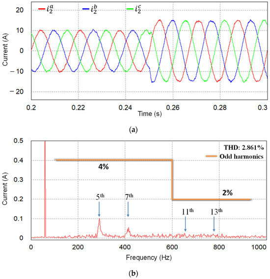
Figure 5.
Simulation results of transient current responses with the proposed scheme under stiff grid and q-axis current reference change at 0.25 s. (a) Grid-side currents; (b) FFT result of a-phase current.
4.2. Performance under Uncertain Grid Impedance
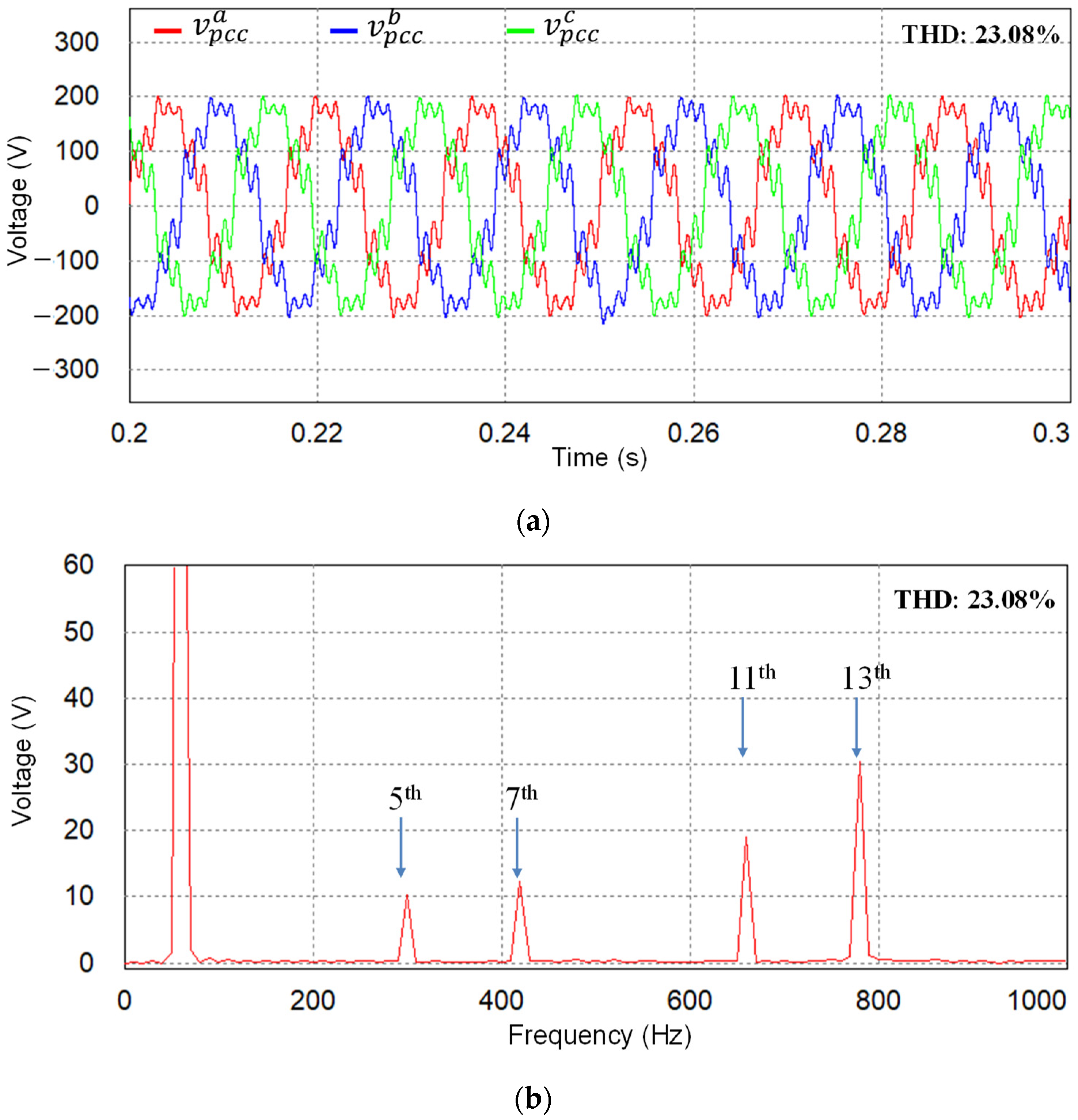
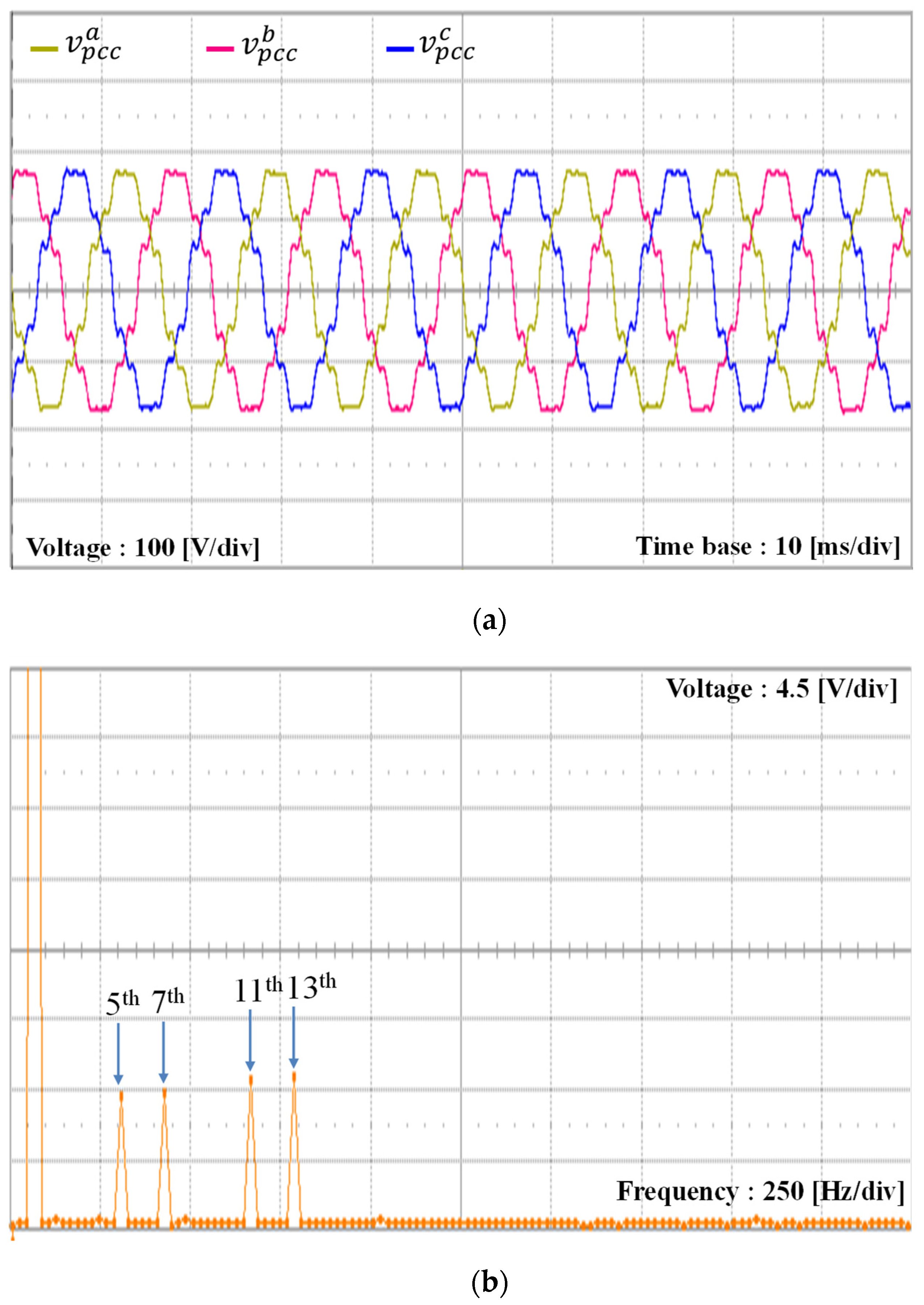
In the next simulations, the proposed scheme is tested under uncertain grid impedances and grid distortion, in which the LC-type and L-type grid impedances are taken into consideration. Figure 6a represents the three-phase PCC voltages when the LC-type grid impedance is linked between the GCI output and the main grid, as shown in Figure 1. As LC-type grid impedance, the grid inductance Lg of 3 mH and grid capacitance Cg of 10 µF are used. Due to the negative effect of the complex grid, the THD level of the PCC voltages increases by 23.08%, and the magnitudes of individual harmonic distortion are also increased, as shown in Figure 6b.
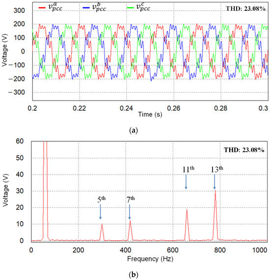
Figure 6.
Three-phase distorted PCC voltages with = 3 mH and = 10 µF. (a) Distorted PCC voltages; (b) FFT result of a-phase voltage.
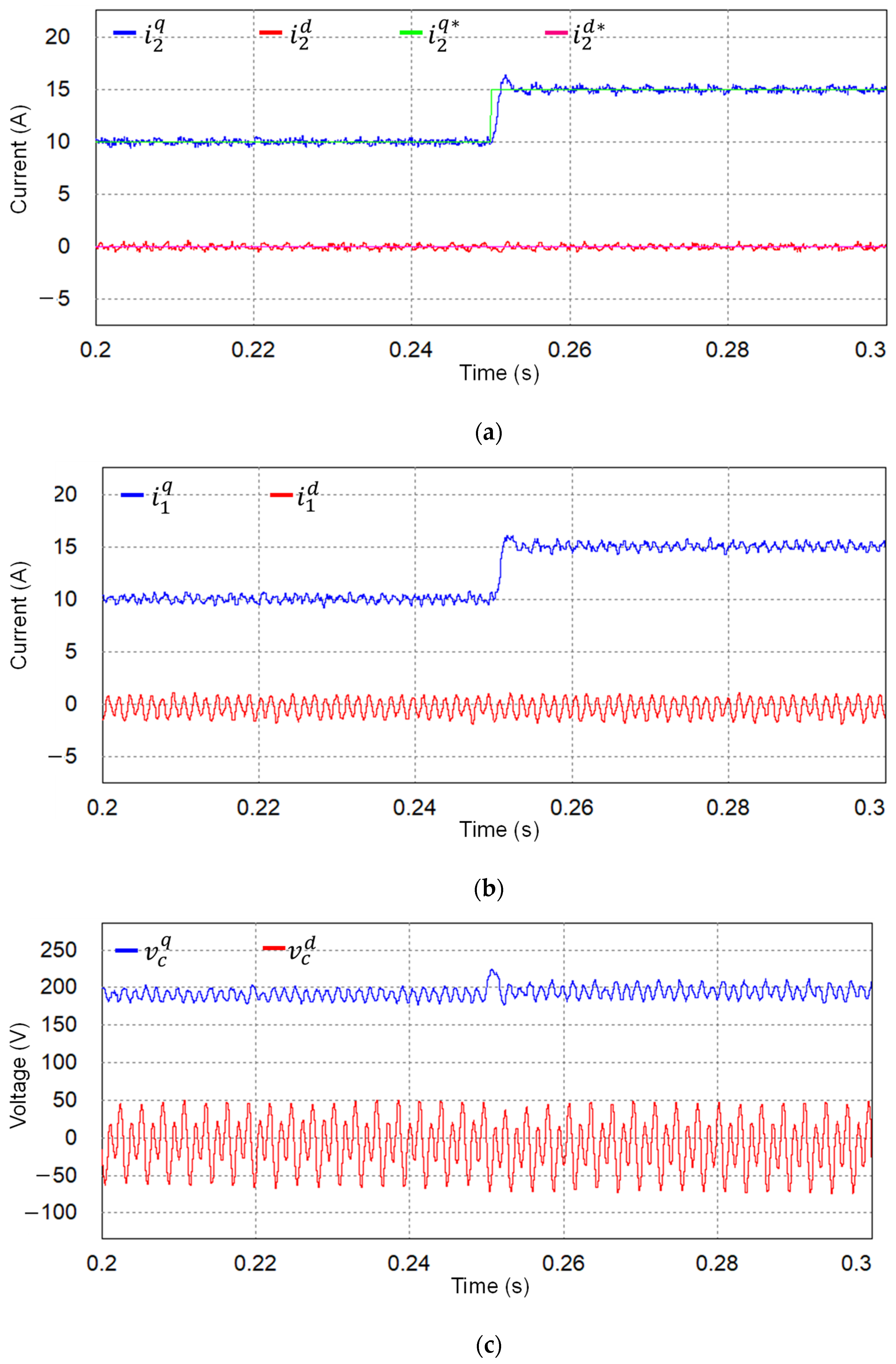
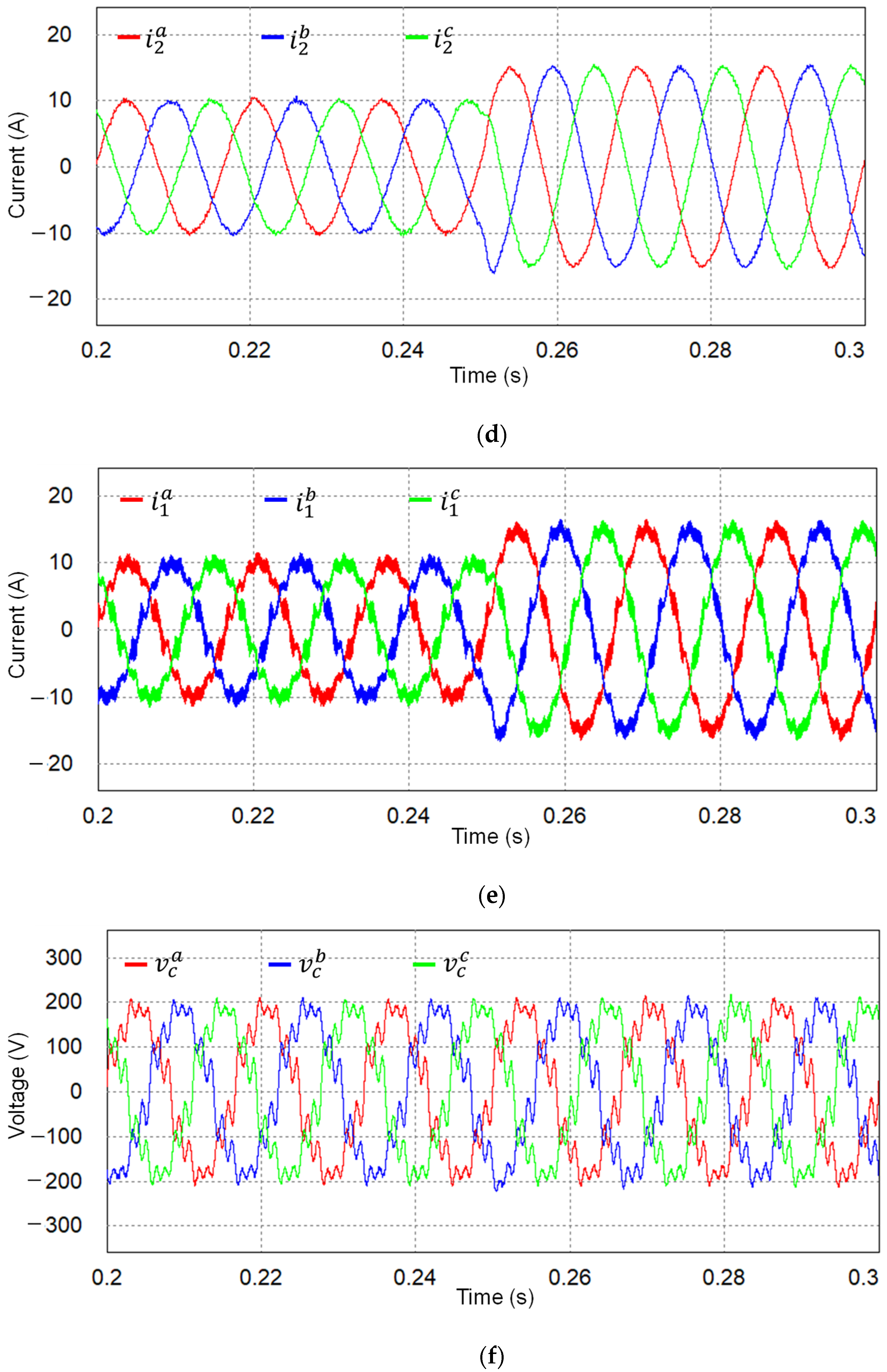
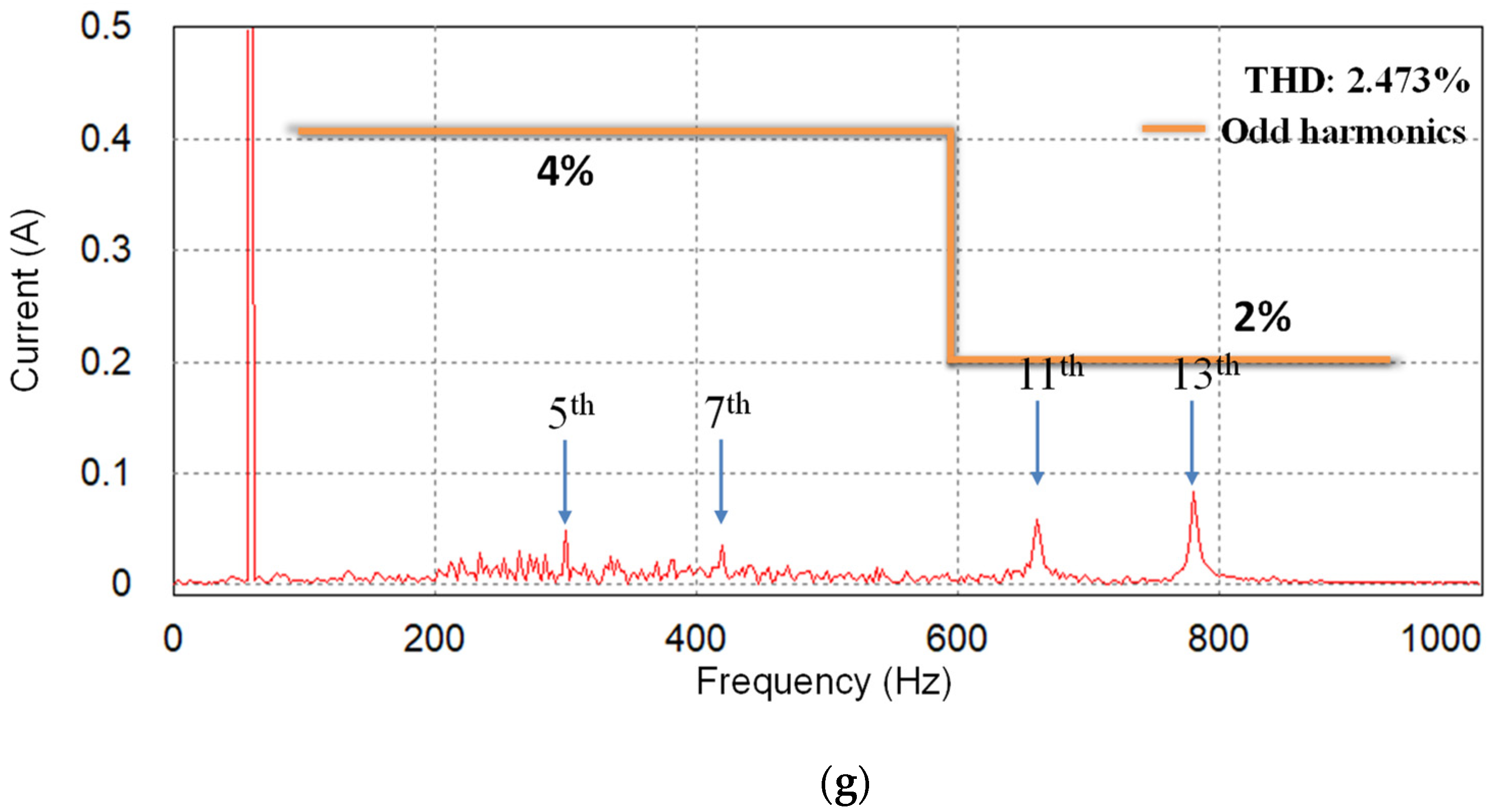
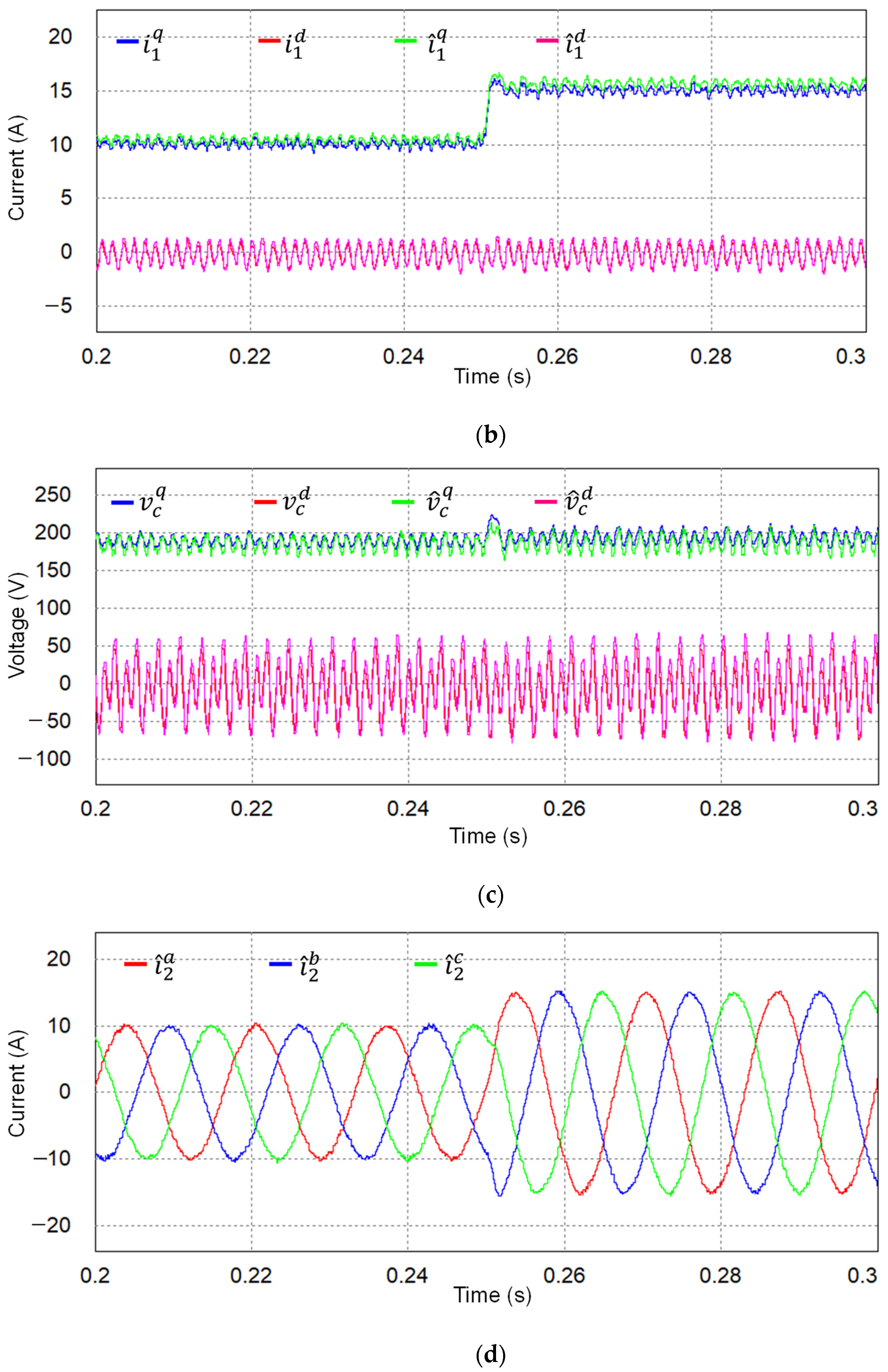
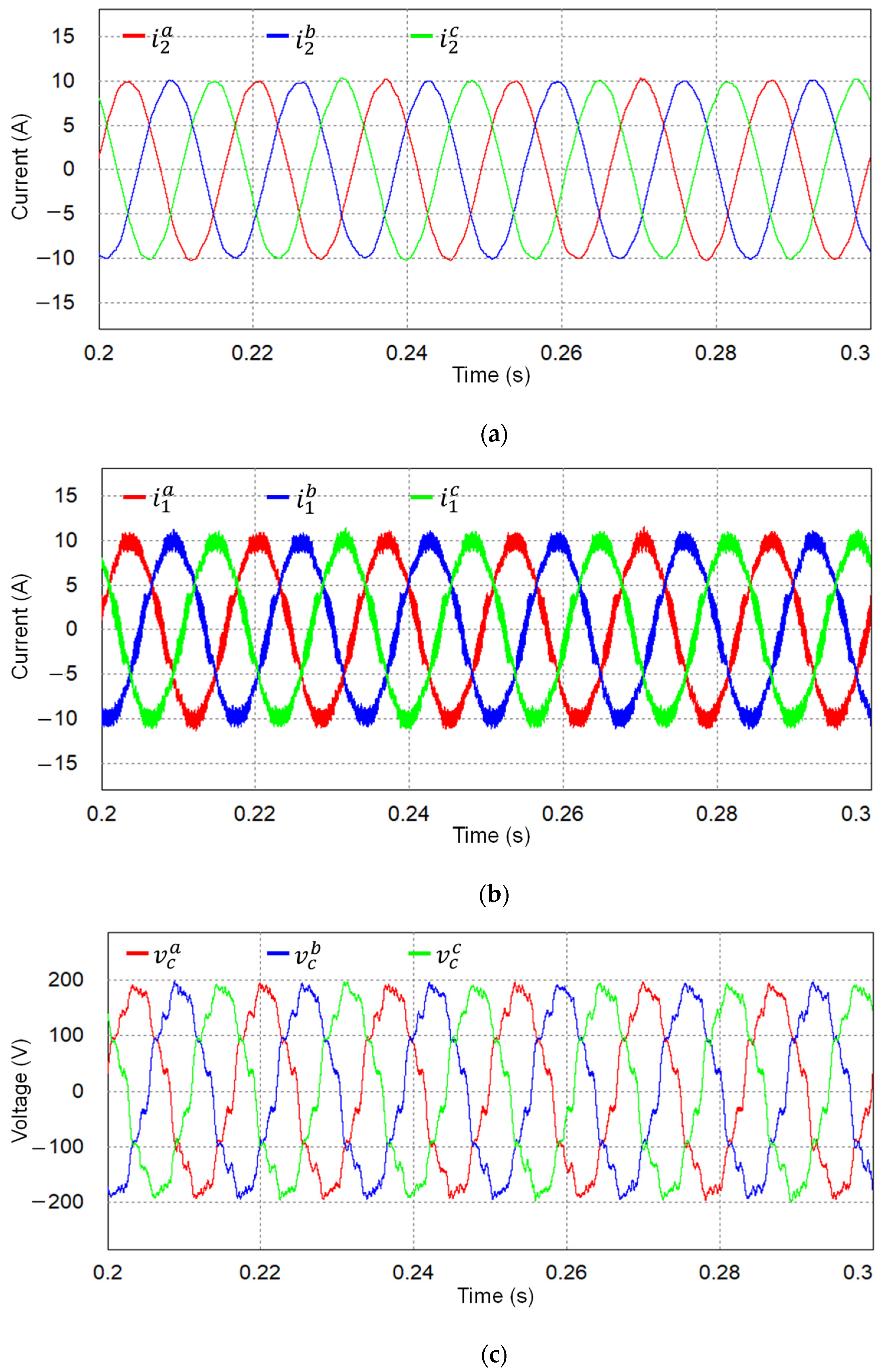
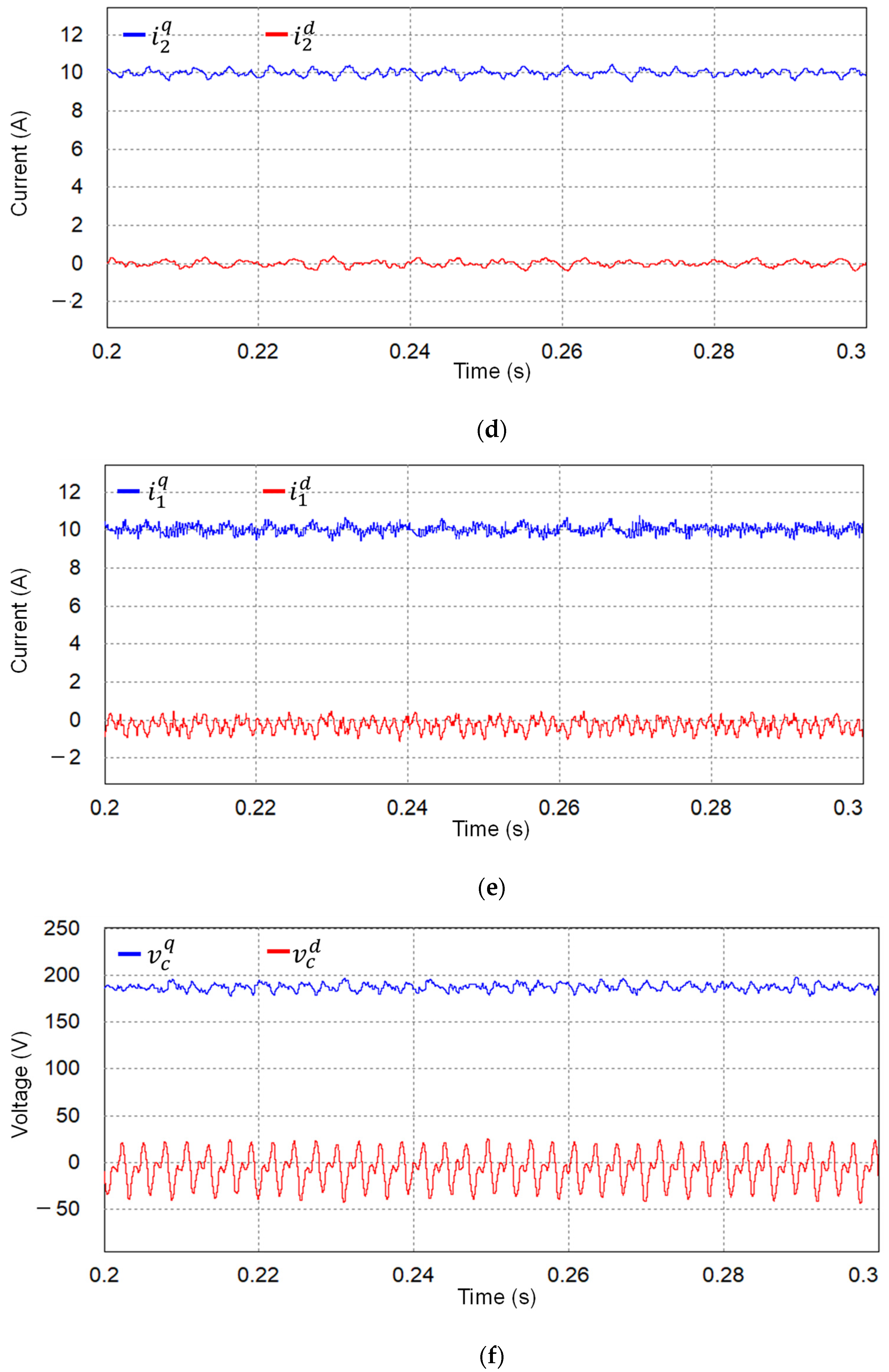
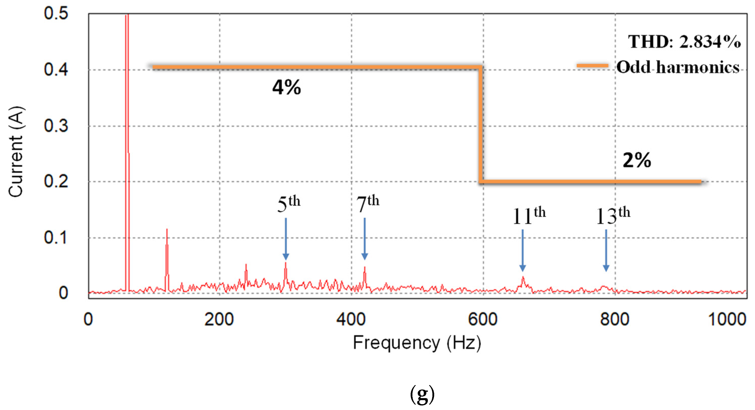
Generally, the grid resonance caused by the complex and distorted grid, as in Figure 6, may severely affect the stability of the GCI control system. To evaluate the performance of the proposed control scheme at steady-state and transient under such conditions, the q-axis current reference is changed at 0.25 s under complex grid conditions in Figure 7. The grid-side currents, inverter-side currents, and capacitor voltages in dq-axes are presented in Figure 7a and Figure 7c, respectively. It is obviously shown that all state variables of the GCI system are maintained stably even at the steady-state or transient stages under the complex grid condition. Also, the grid-side currents shown in Figure 7a follow the references well without a severe overshoot during the transient instant. Three-phase waveforms of state variables are shown in Figure 7d–f. These figures show the three-phase grid-side currents, inverter-side currents, and capacitor voltages, respectively. Lastly, Figure 7g presents the FFT result of a-phase grid-side current at steady-state to confirm the stability and quality of the GCI system under a complex grid. It can be observed that high-order harmonics caused by the LCL filter resonance and the complex grid are effectively damped. Furthermore, low-order distortion harmonics come from the background grid voltages and are maintained as acceptable limits according to the IEEE Std. 1547-2003 [3].
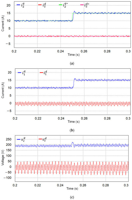
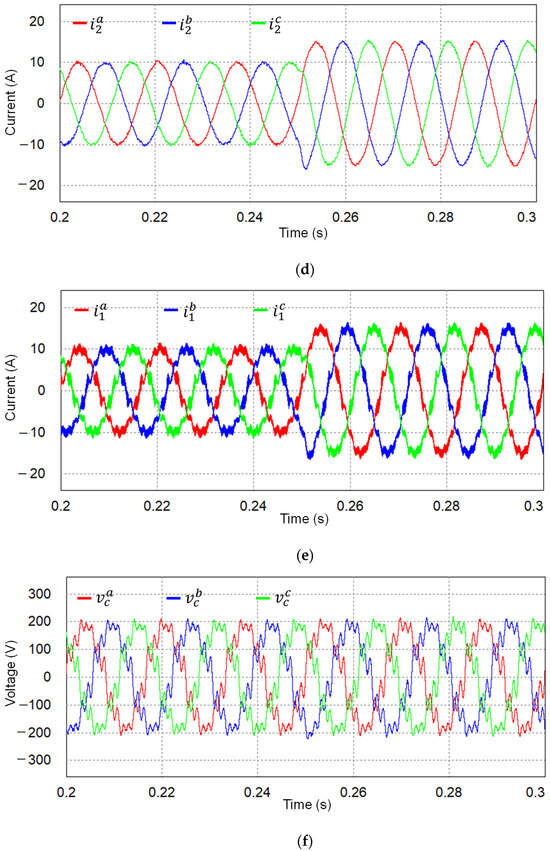
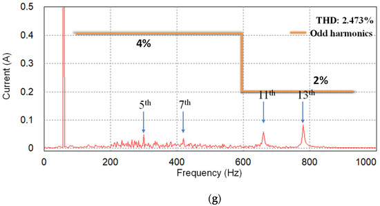
Figure 7.
Simulation results for transient current responses with the proposed scheme when is 3 mH and is 10 µF under q-axis current reference change at 0.25 s. (a) Tracking the performance of grid-side currents at SRF; (b) Inverter-side currents at SRF; (c) Capacitor voltages at SRF; (d) Three-phase grid-side currents; (e) Three-phase inverter-side currents; (f) Three-phase capacitor voltages; (g) FFT result of a-phase grid-side current at steady-state.
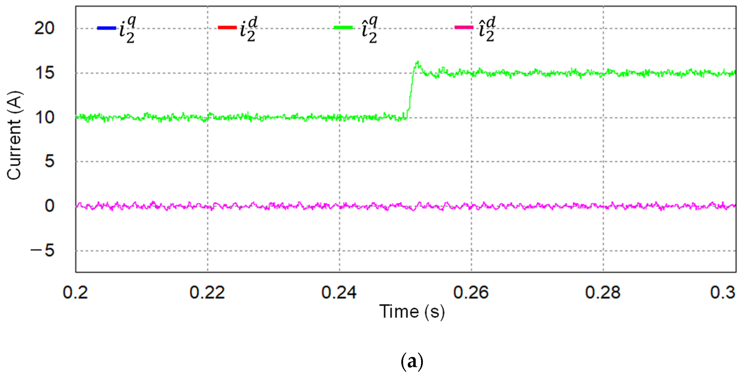
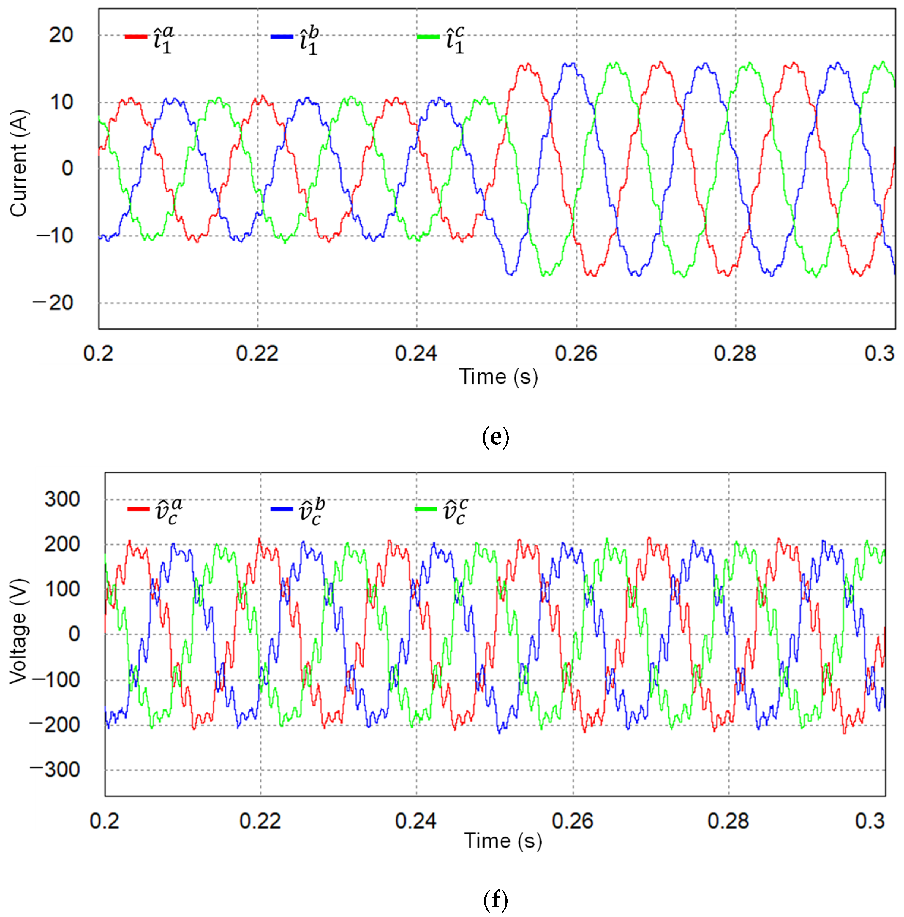
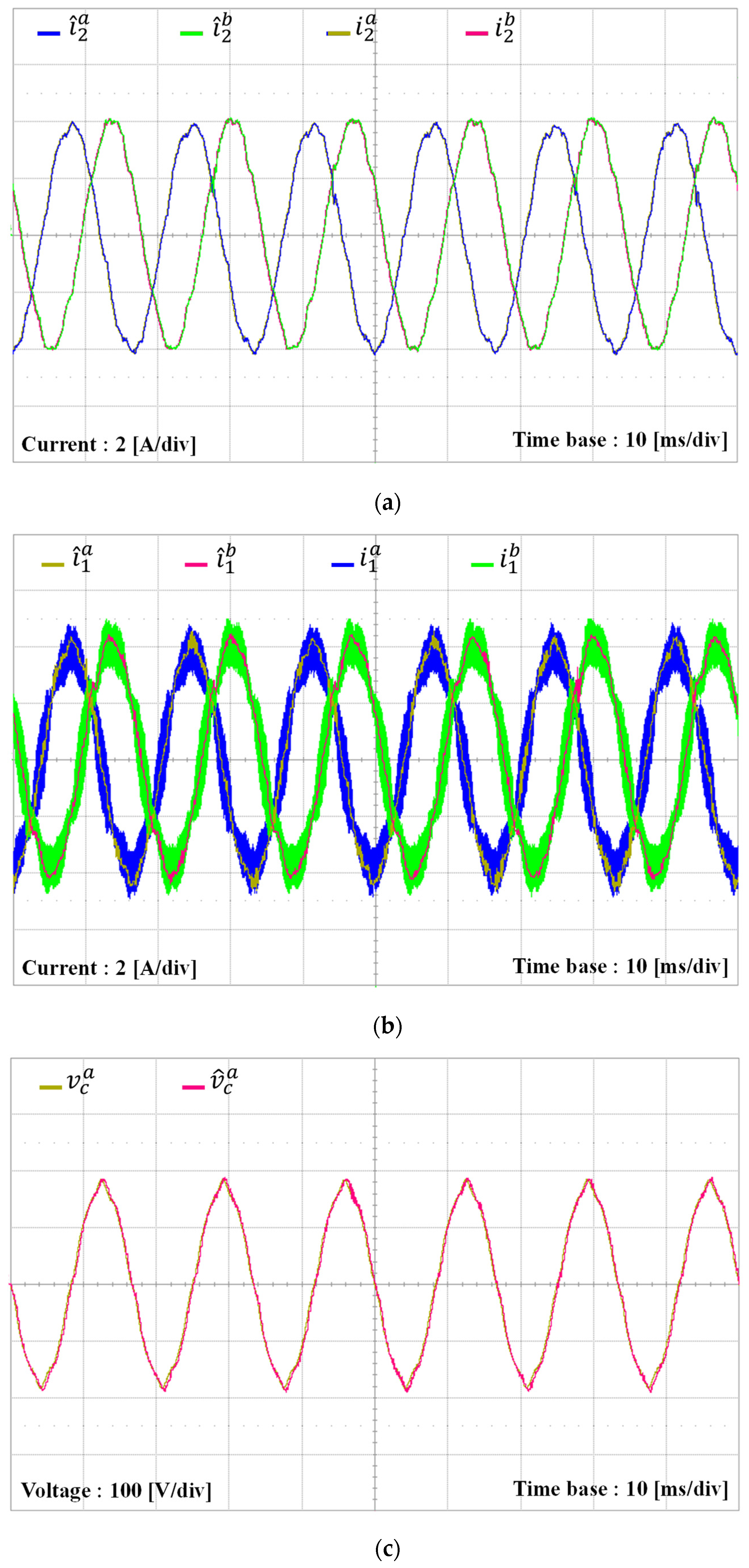
It is worth mentioning again that the proposed control scheme is realized by using only the measurement of the DC-link voltage (VDC), grid-side currents, and PCC voltages. Additional state variables, such as inverter-side current and capacitor voltages, are estimated to construct the proposed state feedback control. To validate the estimating performance of the observer, the simulations are conducted under the same complex grid as in Figure 6. Figure 8a shows the measured and estimated grid-side currents in SRF, in which the estimated state variables track the measured ones exactly. The estimated and measured quantities of inverter-side currents and capacitor voltages are shown in Figure 8b,c, respectively, in which only small steady-state errors are maintained. Thanks to the good performance of the observer, the proposed scheme can produce high-quality grid-side currents and stable operation even under severe grid conditions without the requirement to install full sensing devices. To visualize the estimated state variables in three-phase waveforms, those estimated quantities produced by the observer in SRF are transformed to the natural reference frame as presented in Figure 8d–f. These figures represent the estimated three-phase grid-side currents, inverter-side currents, and capacitor voltages, respectively.
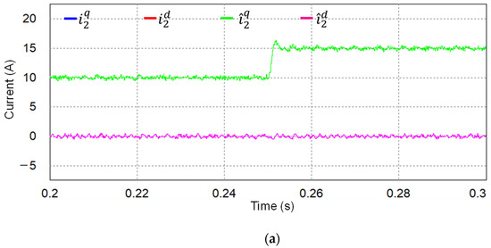
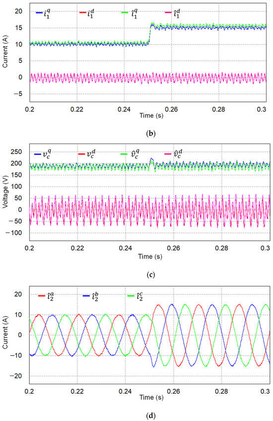
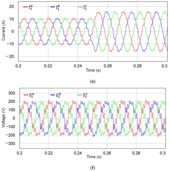
Figure 8.
Simulation results for estimating performance of discrete-time observer when is 3 mH and is 10 µF under q-axis current reference change at 0.25 s. (a) Grid-side currents and estimated states at SRF; (b) Inverter-side currents and estimated states at SRF; (c) Capacitor voltages and estimated states at SRF; (d) Estimated three-phase grid-side currents; (e) Estimated three-phase inverter-side currents; (f) Estimated three-phase capacitor voltages.
Finally, the proposed scheme is evaluated under a distorted grid and the presence of the L-type grid impedance with Lg of 7 mH in Figure 9. Figure 9a,d present high-quality grid-side currents in the natural reference frame and SRF. As is shown in these figures, the currents are injected stably into the main grid. Even though the additional grid inductance Lg affects the dynamics of the GCI system, the GCI still maintains stable operation and the control objectives, such as the reference tracking and disturbance rejection, well by means of the proposed controller. Similarly, the stable inverter-side currents in the natural reference frame and SRF are shown in Figure 9b and Figure 9e, respectively. The capacitor voltages in the natural reference frame and SRF are also plotted in which Figure 9c,f. The quality of injected grid-side currents produced by the proposed scheme is confirmed in Figure 9g, in which the FFT result of a-phase grid-side current is represented together with the harmonics limit specified by the grid code. According to the frequency analysis, all the harmonic components of the grid current are less than the limit, and the THD level is only 2.834%.
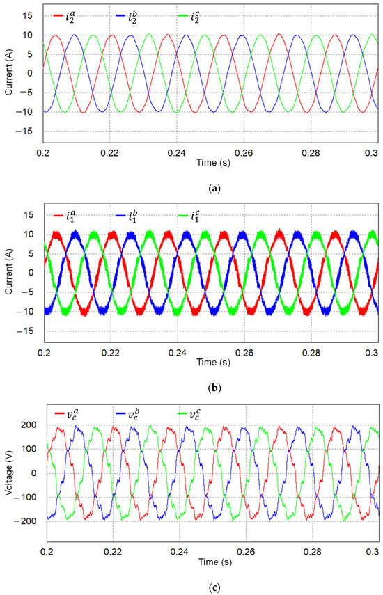
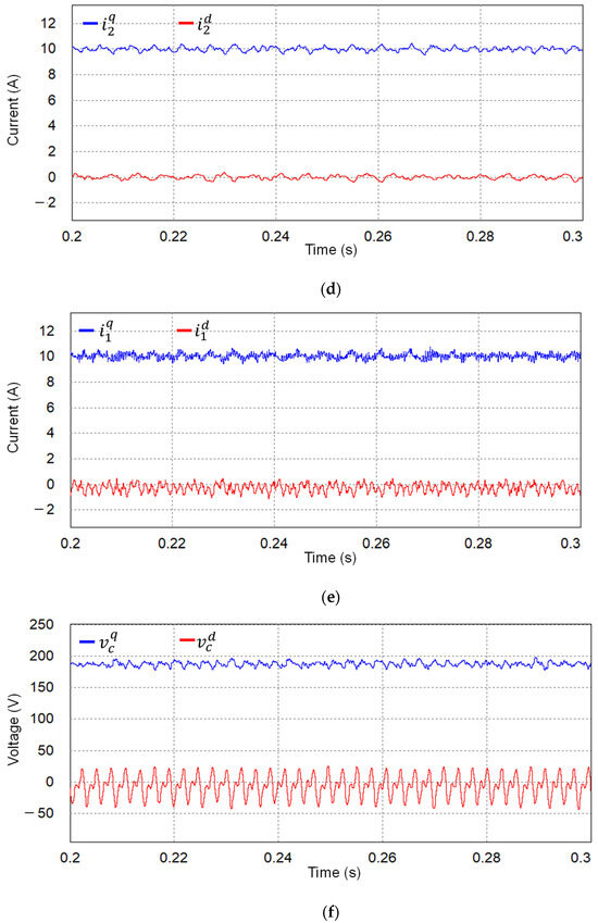

Figure 9.
Simulation results for the proposed scheme when is 7 mH. (a) Grid-side currents; (b) Inverter-side currents; (c) Capacitor voltages; (d) Grid-side currents at SRF; (e) Inverter-side currents at SRF; (f) Capacitor voltages at SRF; (g) FFT result of a-phase grid-side current.
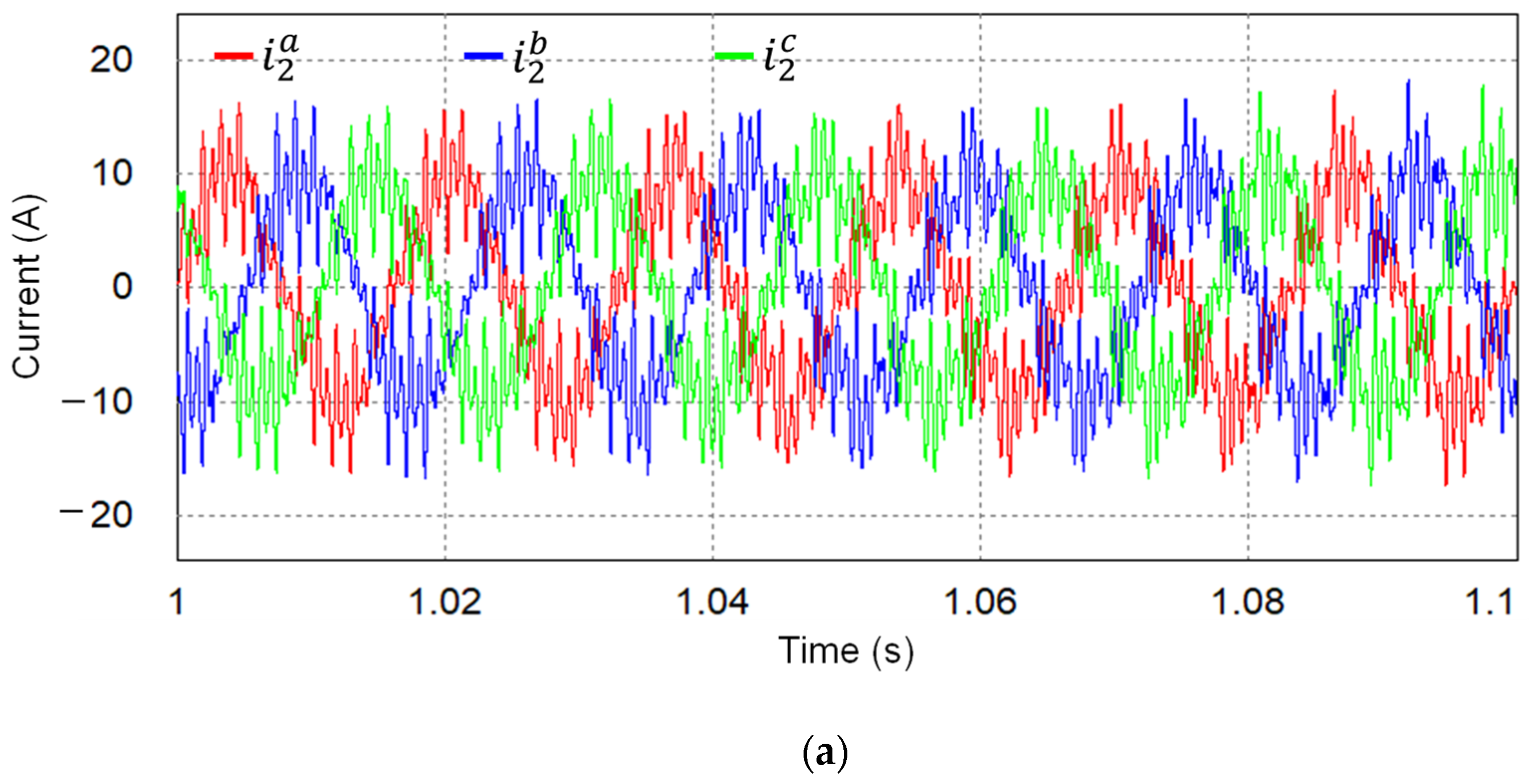
To demonstrate the effectiveness of the proposed control scheme as compared to the existing control scheme, the comparative simulations are performed by using the control scheme in [22] under the same conditions of the LC-type grid impedance and grid distortion as in Figure 6. Figure 10a,b show three-phase current responses and the FFT result of a-phase current by the controller in [22], respectively. Even if this control scheme shows a desirable performance initially, it becomes unstable with significant oscillation of currents and a high THD level of 69.94% as time goes on. On the contrary, Figure 11a,b represent three-phase current responses and the FFT result of the a-phase current by the proposed current controller with the same test condition as Figure 10. Thanks to the consideration of the LC grid impedance in the design process, stable injected currents can be maintained, as shown in Figure 11. The above fair comparison results clearly highlight the superior performance of the proposed current controller under LC-type grid impedance.
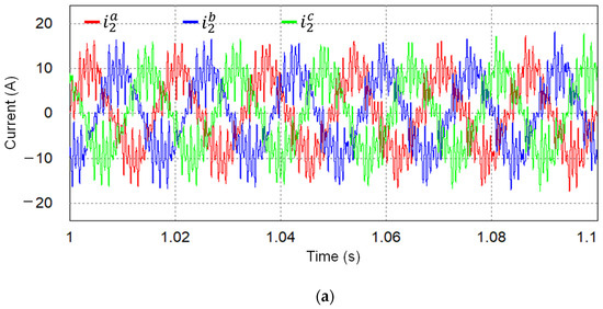
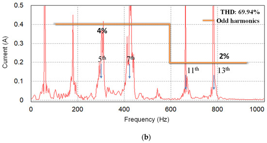
Figure 10.
Simulation results for the control scheme in [22] when is 3 mH and is 10 µF. (a) Grid-side currents; (b) FFT result of a-phase grid-side current.
Figure 11.
Simulation results for the proposed control scheme when is 3 mH and is 10 µF. (a) Grid-side currents; (b) FFT result of a-phase grid-side current.
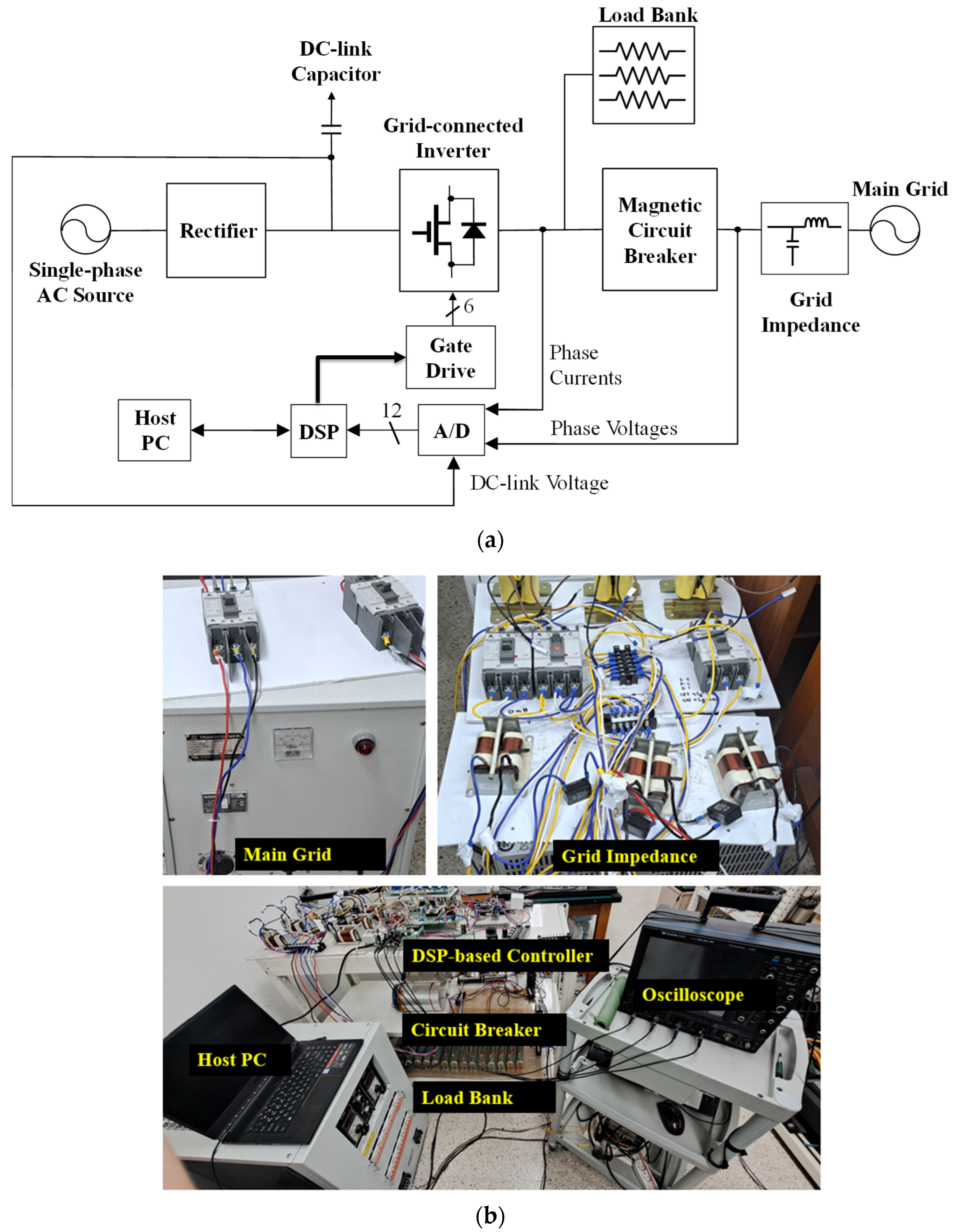
5. Experimental Results
To validate the feasibility of the proposed scheme, the experiments are conducted on a lab-based prototype system of three-phase GCI, as shown in Figure 12. To control the three-phase LCL-filtered GCI prototype, the proposed scheme is executed on the digital signal processor (DSP) TMS320F28335 (Texas Instruments, Dallas, TX, USA) with the measurements of the DC-link voltage, grid currents, and grid voltages. All the measurements from the sensors are processed with a 12-bit analog-to-digital (A/D) converter to send the information to DSP. The schematic of the overall system is shown in Figure 12a, in which the system parameters of the experimental prototype are listed in Table 1. The photograph of the experimental setup is also shown in Figure 12b.
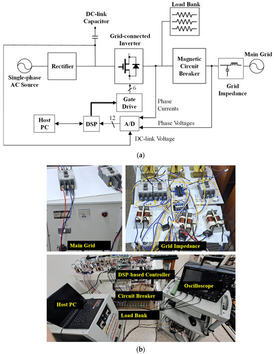
Figure 12.
Experimental configuration. (a) Schematic of the overall system; (b) Photograph of the experimental setup.
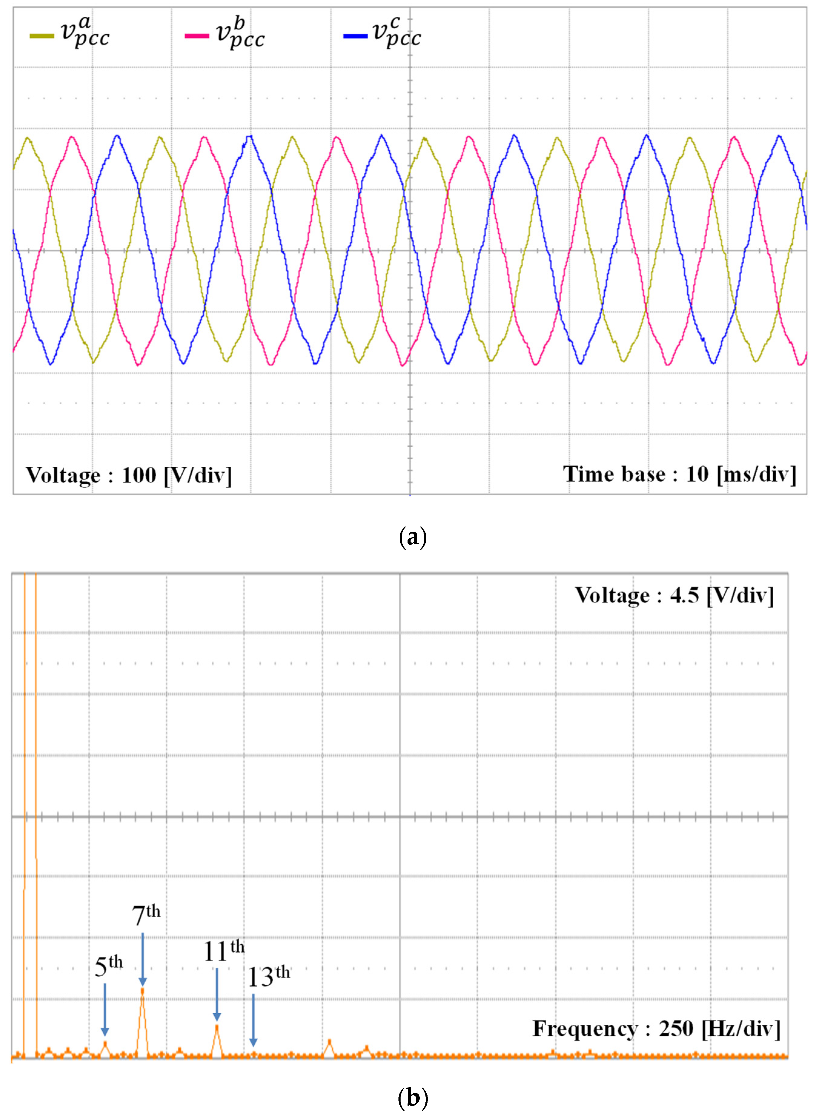
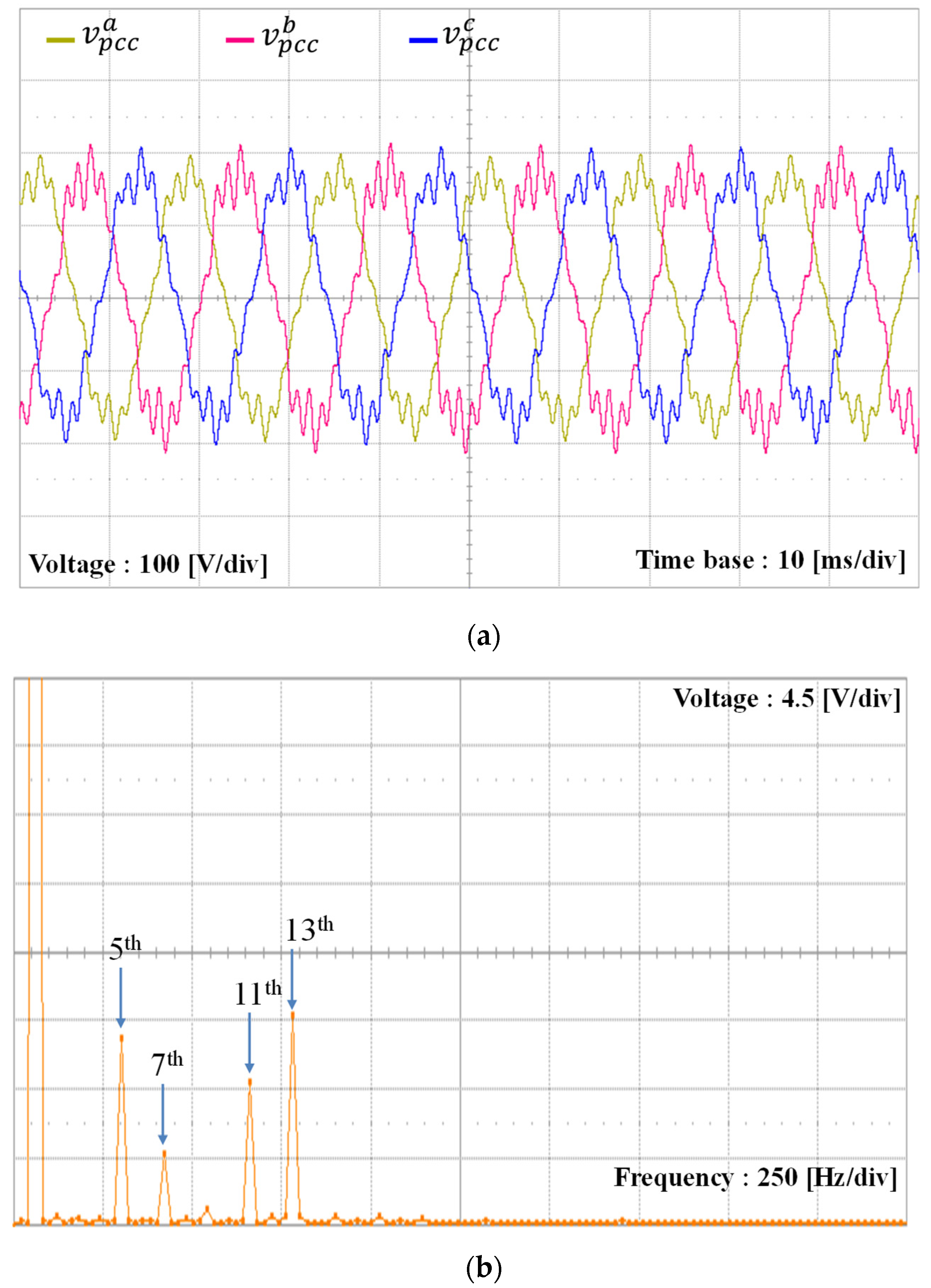
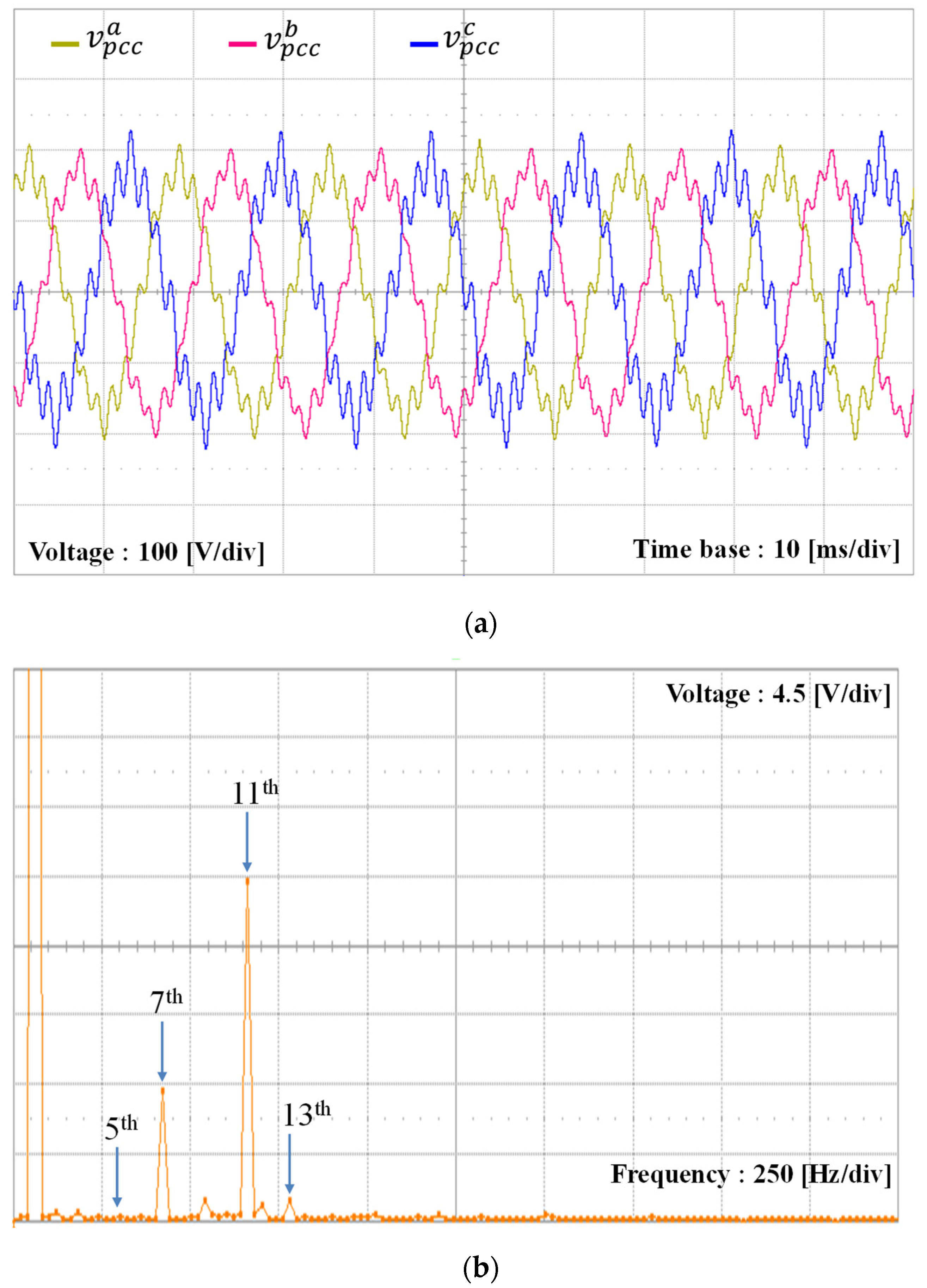
Figure 13a shows the three-phase main grid voltages used for the experiments. In this case, the grid voltages and PCC voltages are the same since there are no grid impedances. It is clearly shown that the real main grid inevitably includes harmonic distortions. The FFT result of a-phase PCC voltage (real grid voltage) shown in Figure 13b shows large harmonic components at 7th and 11th orders with small components in other low-order harmonics.
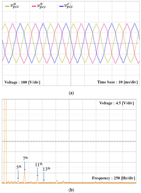
Figure 13.
PCC voltages were used for the experiments. (a) Distorted PCC voltages; (b) FFT result of a-phase PCC voltage.
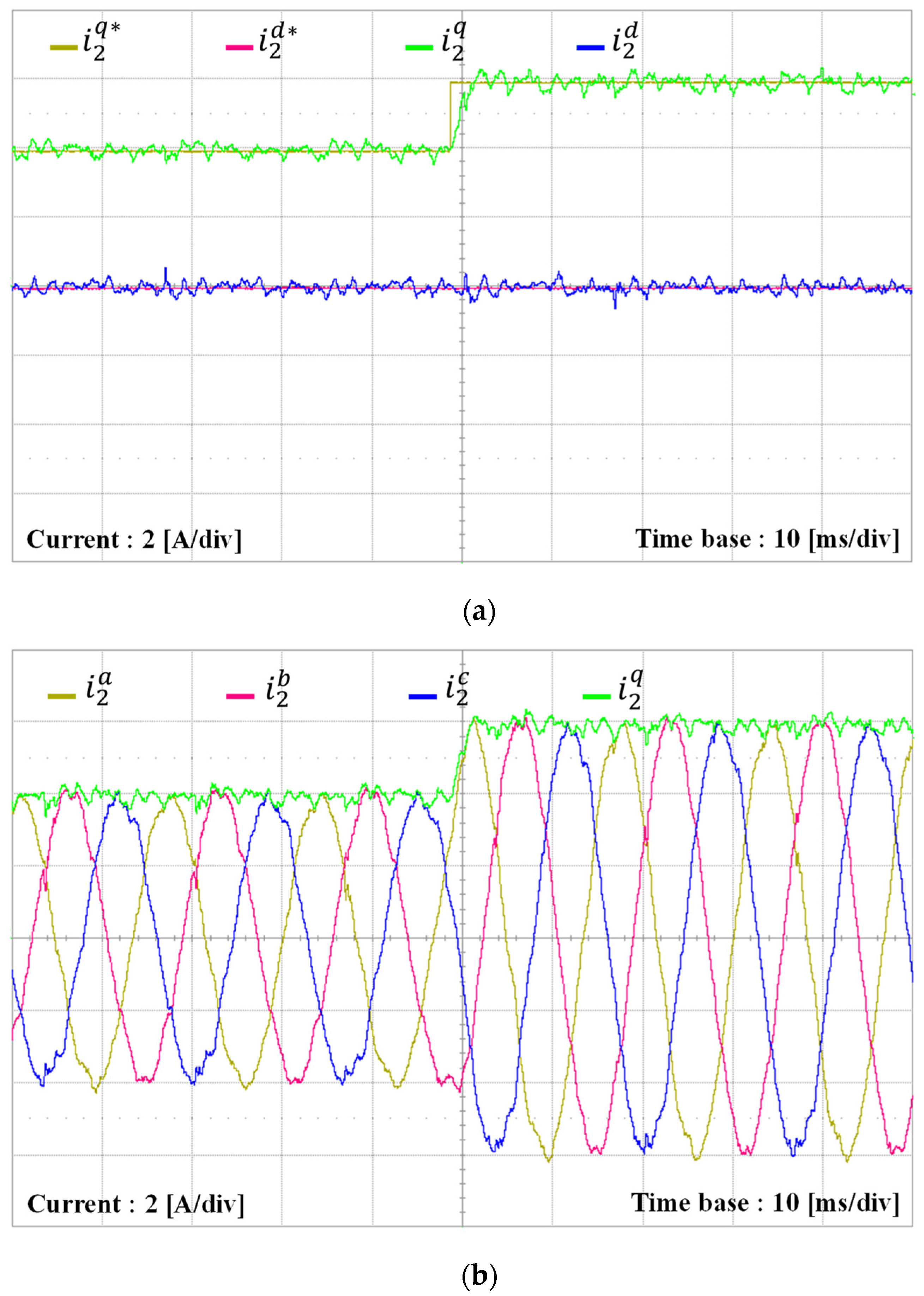
The first experiment is conducted to verify the tracking performance of the proposed control scheme in the SRF under a stiff grid. Figure 14 shows the experimental results for transient responses of grid-side currents under a distorted grid environment and the step change in q-axis current reference from 4 A to 6 A. The grid-side current waveforms in SRF and natural reference frames are presented in Figure 14a,b, respectively. It is obvious from this test result that the grid-side currents rapidly track new references with quite negligible overshoot, which agrees well with the simulation in Figure 5.
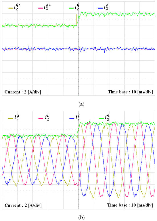
Figure 14.
Experimental results for transient responses with the proposed scheme under step change in q-axis current reference. (a) Tracking the performance of grid-side currents in SRF; (b) Grid-side currents.
Figure 15 shows the experimental results with the proposed scheme for grid-side current waveforms at steady-state under a distorted grid. It is observed that the effect from distorted harmonics in the background grid is well reduced on the injected currents, which yields considerably sinusoidal grid-side current waveforms, as shown in Figure 15a. To confirm that requirements for the harmonic limits of grid-side currents satisfy the IEEE Std. 1547, the FFT result for a-phase grid current is presented in Figure 15b. The FFT analysis result shows that the harmonic components are significantly attenuated in output currents.
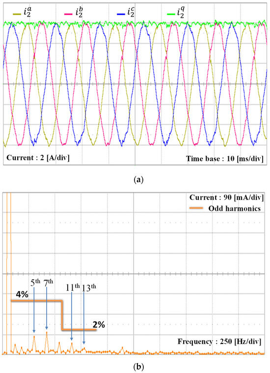
Figure 15.
Experimental results for steady-state responses with the proposed scheme. (a) Grid-side currents and q-axis current; (b) FFT result of a-phase grid-side current.
To validate the estimating performance of observer, estimated and measured quantities of each state variable are presented. Figure 16a–c show the comparison of the estimated and measured states for the grid-side currents, inverter-side currents, and capacitor voltages, respectively. Those experimental results clearly show that the estimated quantities track well their measured ones with a good accuracy.
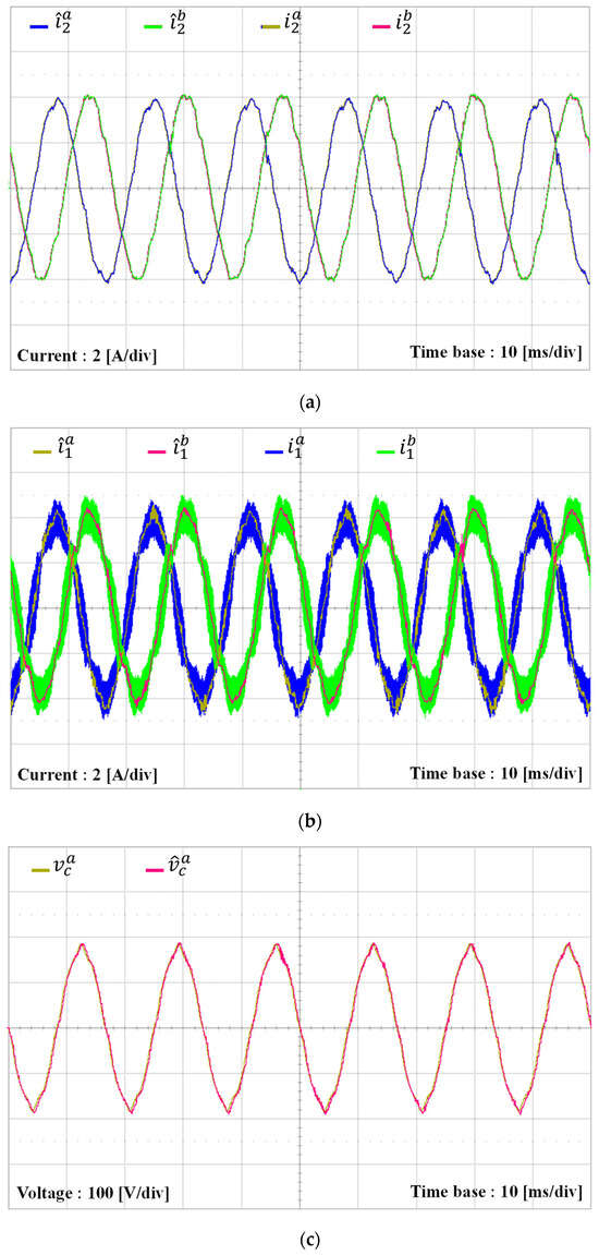
Figure 16.
Experimental results for estimating the performance of the observer. (a) Comparison of the estimated and measured grid-side currents; (b) Comparison of the estimated and measured inverter-side currents; (c) Comparison of the estimated and measured capacitor voltages.
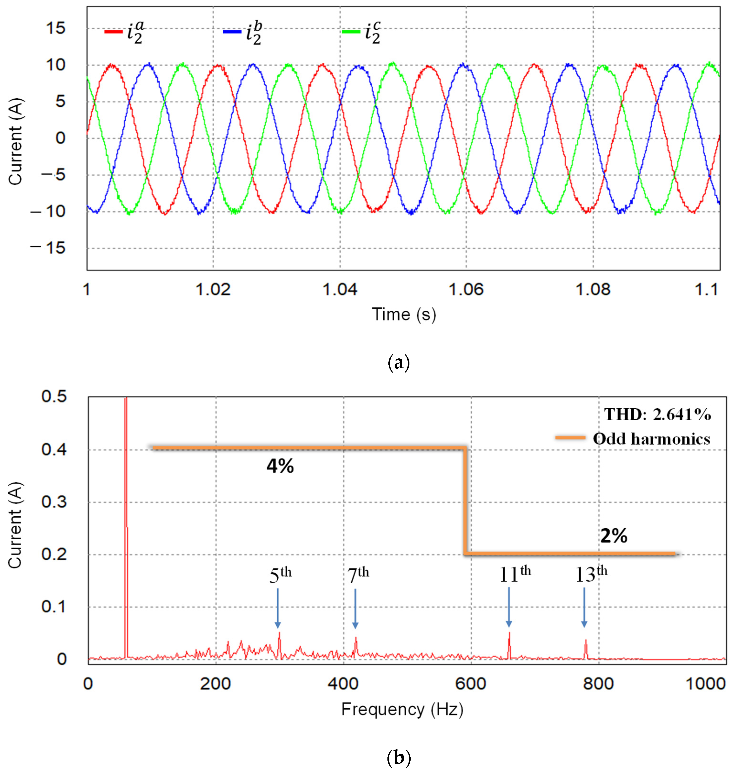
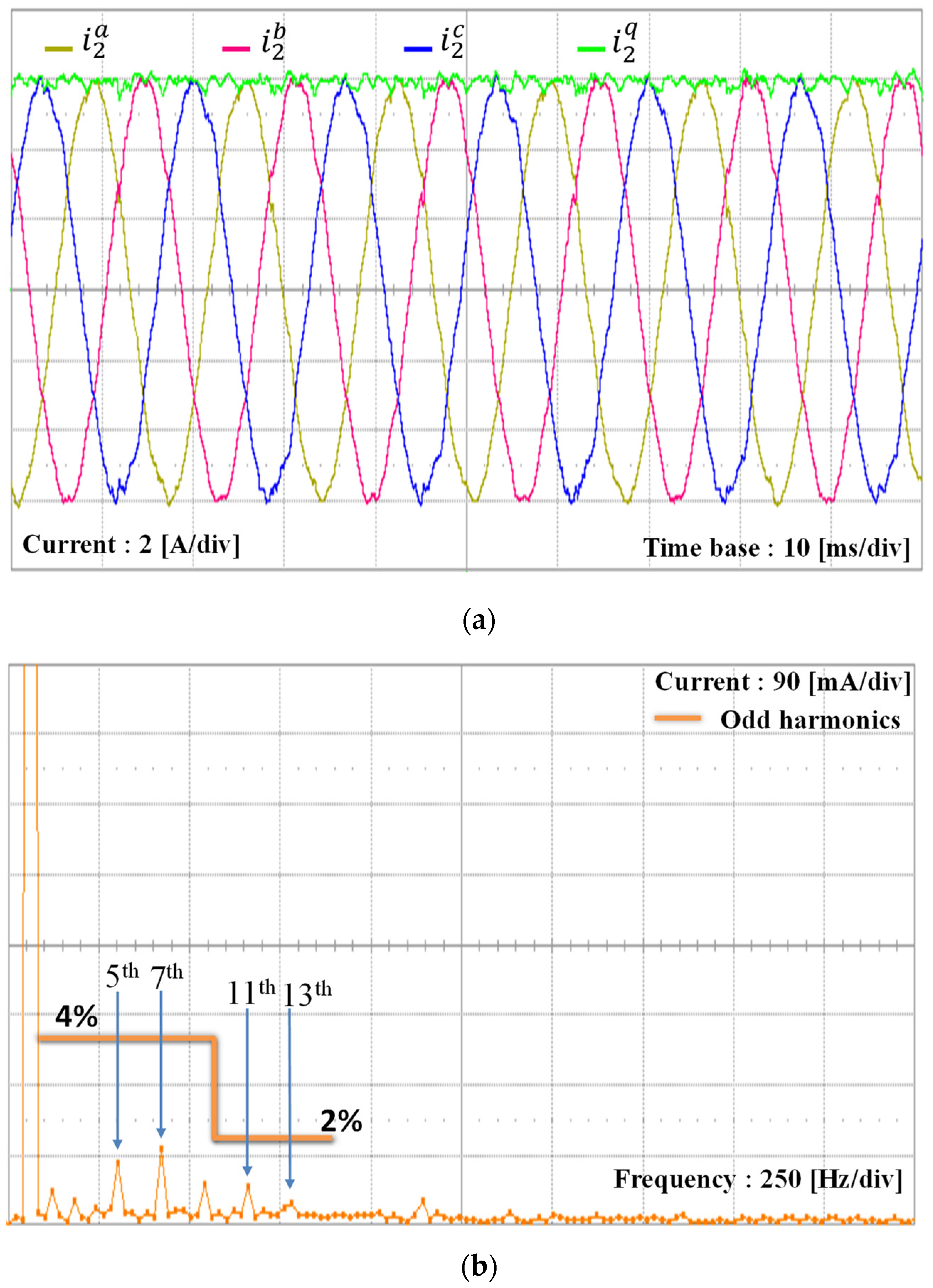
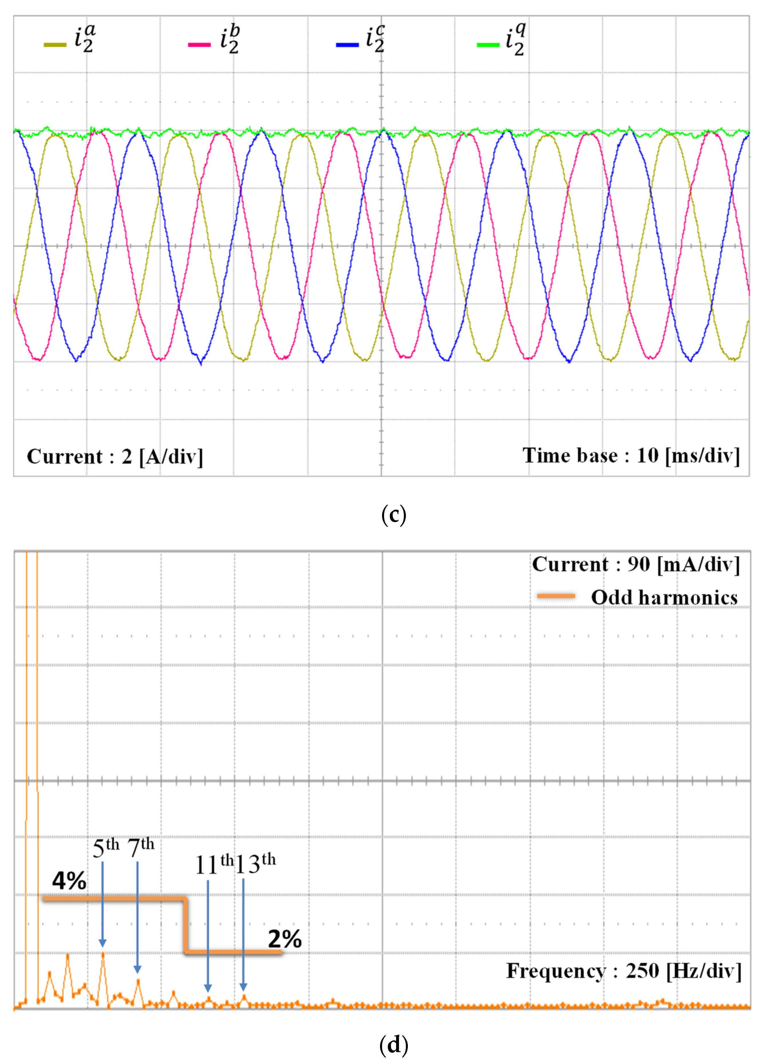
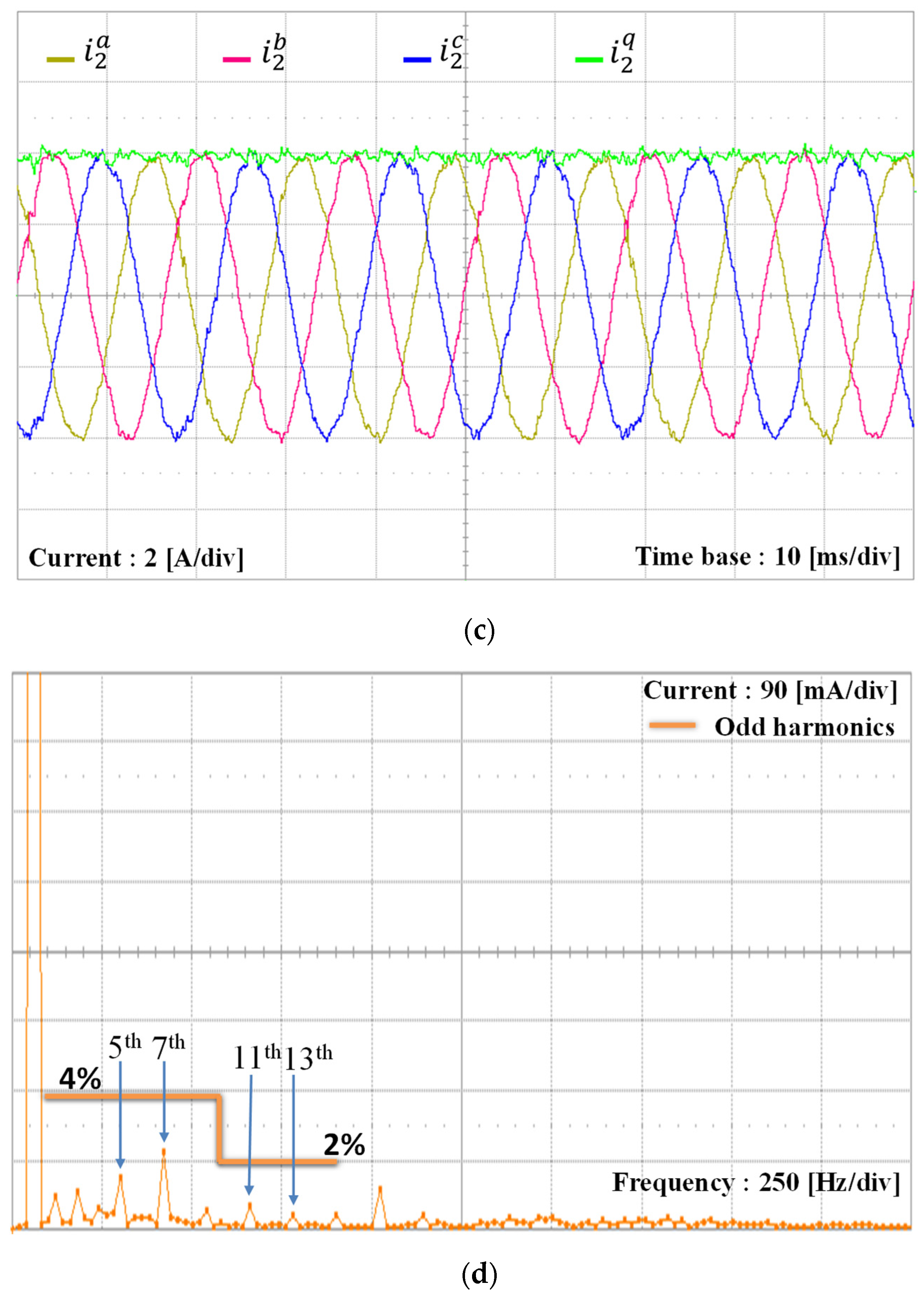
To investigate the performance of the inverter controlled by the proposed control scheme under severe grid distortion, the experiments are performed with low-order grid distortion harmonics at 5th, 7th, 11th, and 13th, in which the distortion level of each harmonic is set to 5% of the fundamental component of the nominal grid magnitude. To assign the above grid distortion level, a programmable AC power source is used instead of the real main grid. Figure 17 shows a three-phase main grid under severe grid conditions. In this case, the grid voltages and PCC voltages are also the same because there are no grid impedances like Figure 13. Figure 18 shows the experimental results with the proposed current control scheme for three-phase grid-side current waveforms at steady-state when the q-axis current reference is 4 A under severely distorted grid conditions. As is shown in Figure 18a, high-quality grid-injected currents can also be obtained by the proposed control scheme due to a good harmonic disturbance compensation. The FFT result of the a-phase grid current presented in Figure 18b also confirms high-quality currents.
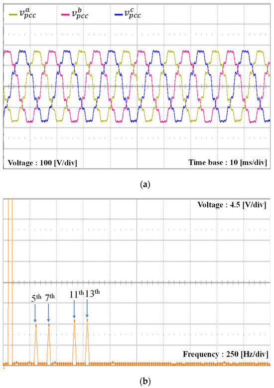
Figure 17.
PCC voltages were used for the experiments. (a) Distorted PCC voltages; (b) FFT result of a-phase PCC voltage.

Figure 18.
Experimental results for steady-state responses with the proposed control scheme. (a) Grid-side currents and q-axis current; (b) FFT result of a-phase grid-side current.
To validate the robustness of the proposed scheme under the grid impedance variations, several experiments are conducted when L-type or LC-type grid impedance exists under the distorted grid environment.
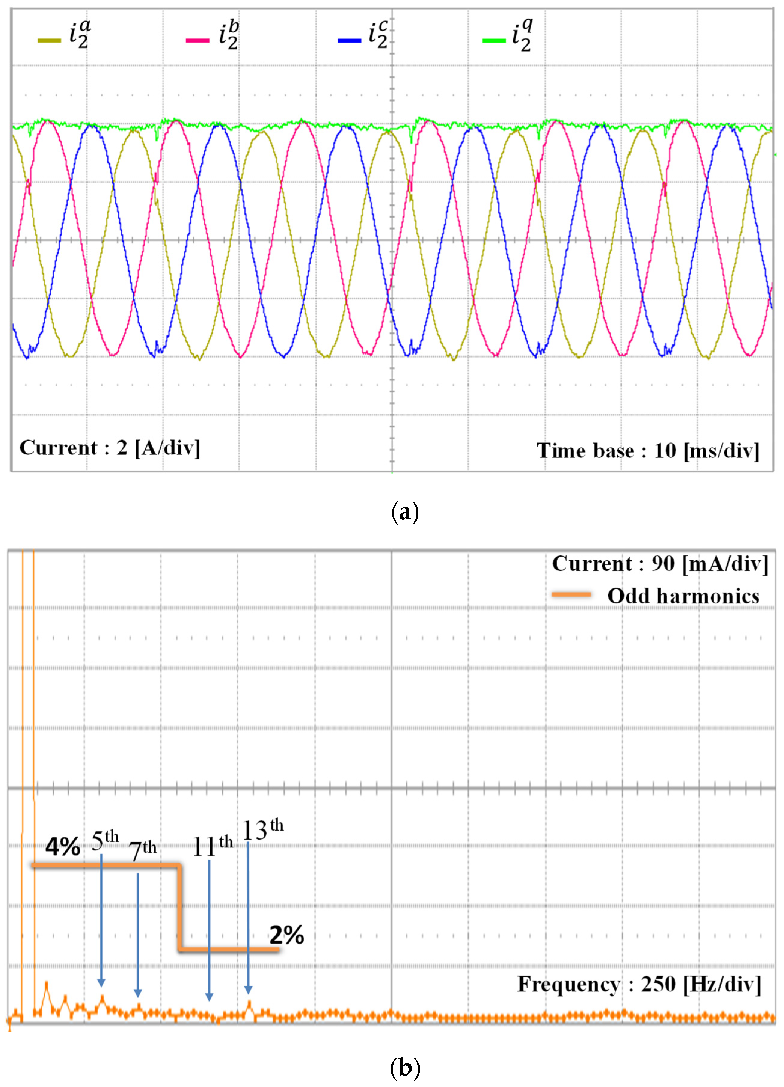
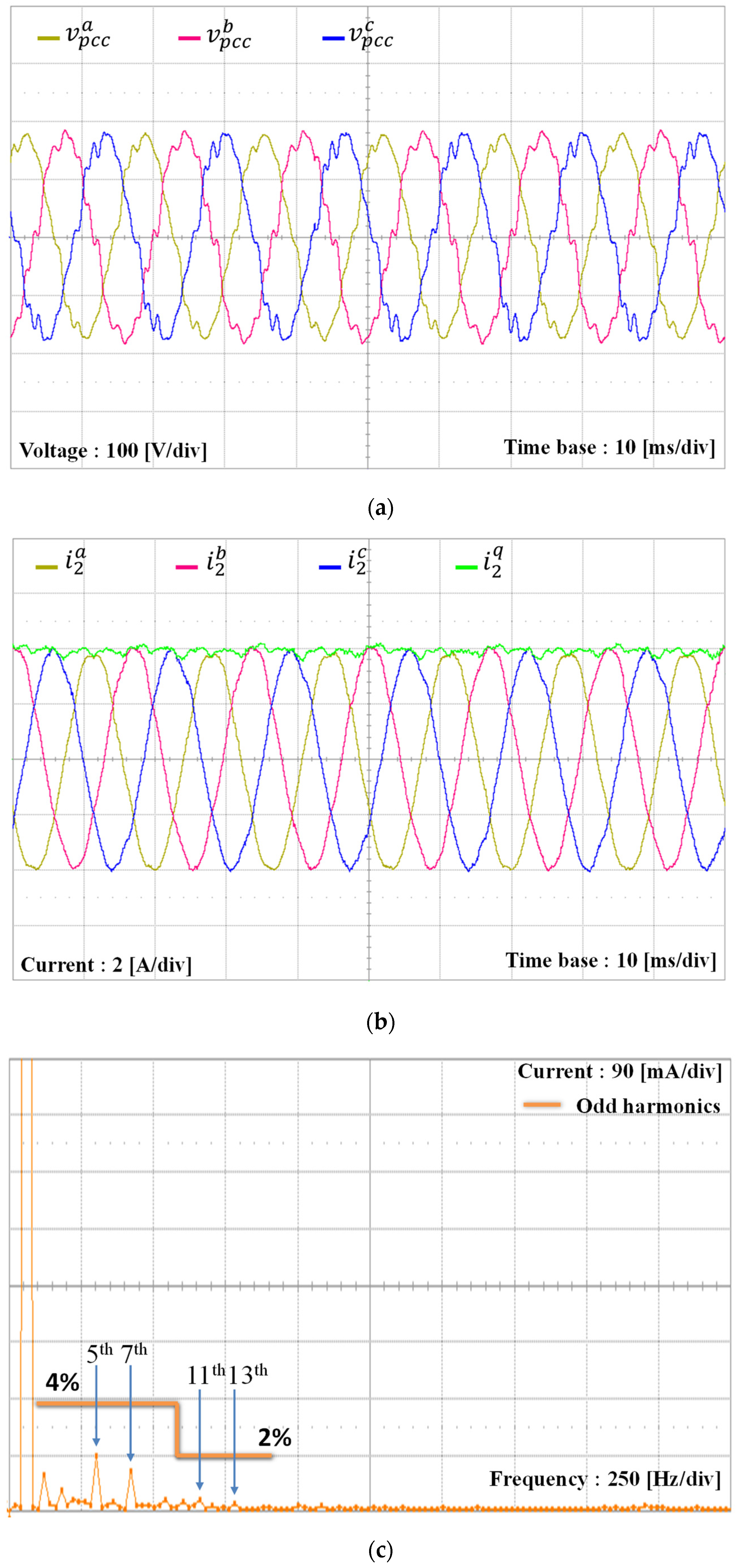
As the first experimental test, the GCI system controlled by the proposed scheme is operated under the existence of an uncertain grid inductance of 5 mH. Due to the additional grid inductance, the distortion level of three-phase PCC voltages shown in Figure 19a is increased as compared to Figure 13a. To comprehensively present the performance of the proposed current controller, three-phase grid-side and q-axis grid-side currents are presented in the same graph of Figure 19b. The current responses clearly show stable and sinusoidal grid-side currents under L-type grid impedance. Also, the good tracking performance of the q-axis grid-side current is confirmed by the q-axis current response. Lastly, the FFT result of a-phase grid-side current is plotted in Figure 19c to show the distortion level of the current. Not only are the low-order distortion harmonics caused by the distorted grid environment well compensated, but the high-order resonant frequencies are also well-damped. These results clearly show that the control objectives and the stable operation of the GCI system controlled by the proposed control scheme are still maintained under L-type grid impedance.
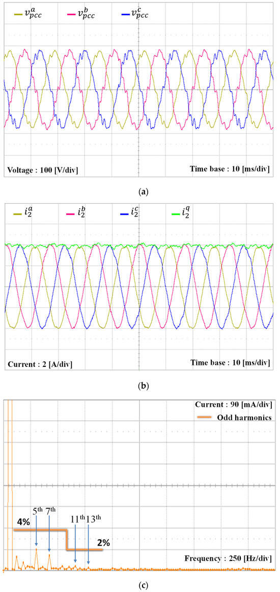
Figure 19.
Experimental results for the proposed scheme when uncertain grid inductance of 5 mH exists. (a) Distorted PCC voltages; (b) Grid-side currents and q-axis current; (c) FFT result of a-phase grid-side current.
To verify the alignment between the simulation and experimental results of the proposed scheme under the L-type grid impedance, the grid inductance is increased to 7 mH, which is similar to the simulation setup in Figure 9. Due to the increase of the grid inductance, the PCC voltages are distorted further by increased magnitudes of low-order harmonics, as shown in Figure 20a. As shown in Figure 20b, the harmonic components in the orders of 5th, 7th, 11th, and 13th are 6.9%, 2.5%, 5%, and 7.5% of the fundamental grid voltage magnitude, respectively. Even under such severe conditions, three-phase grid-side currents of the GCI controlled by the proposed scheme in Figure 20c,d show high-quality grid-injected currents similar to Figure 9.
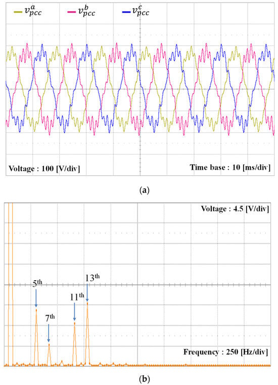
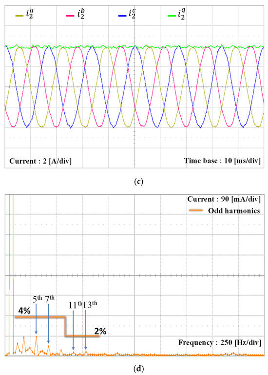
Figure 20.
Experimental results for the proposed scheme when the grid inductance is increased to 7 mH. (a) Distorted PCC voltages; (b) FFT result of a-phase PCC voltage; (c) Grid-side currents; (d) FFT result of a-phase grid-side current.
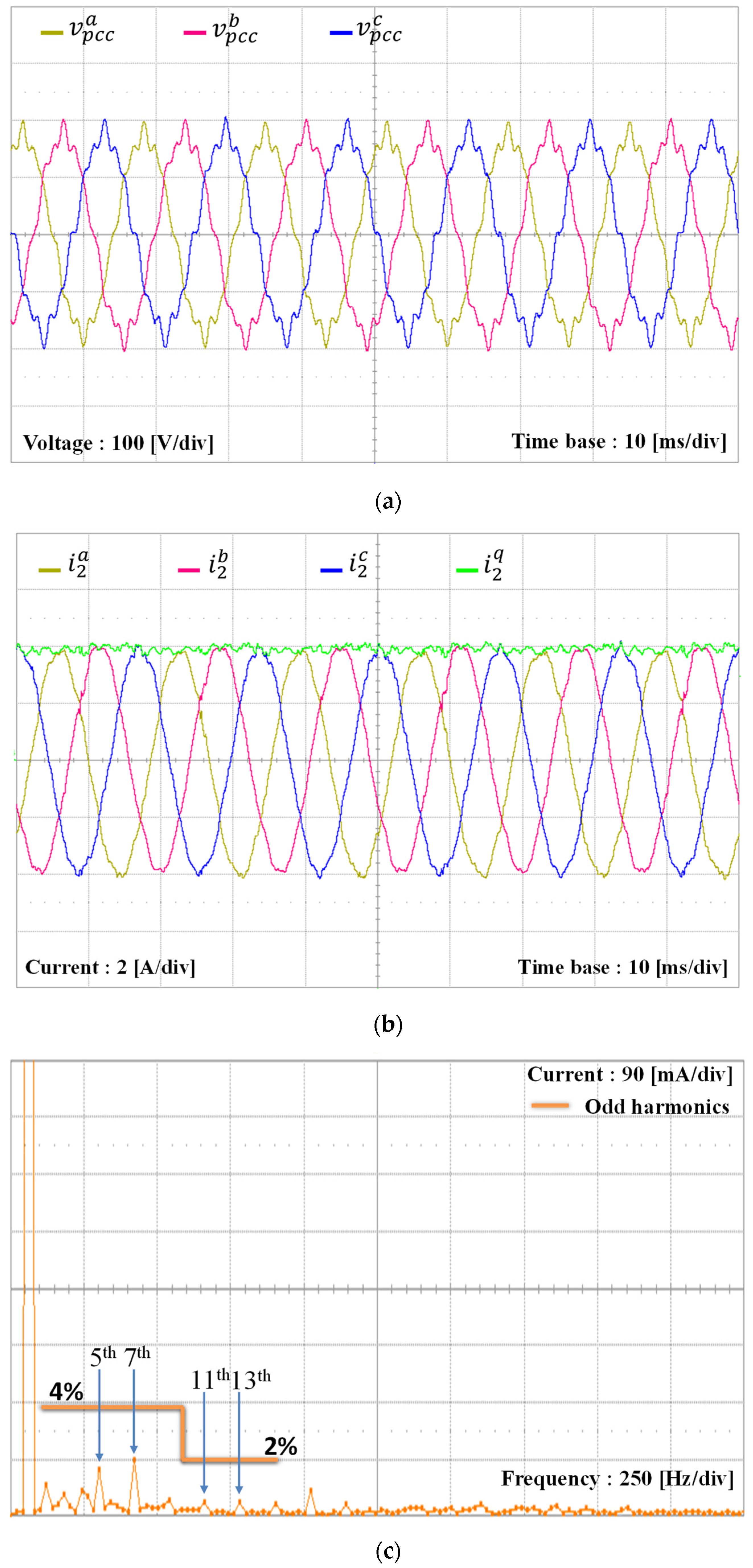
In the next tests, the GCI system is operated under the complex grid, in which the LC-type grid impedances are connected between the GCI output and the main grid. In Figure 21, the grid impedance is set with the grid inductance Lg of 3 mH and the grid capacitance of 8 µF. The q-axis reference current is applied as 4 A to validate the performance of the proposed scheme under a complex grid. As shown in Figure 21a, the additional LC-type grid impedance causes the distortion increment in the PCC voltages as well. Even under this severe complex grid condition, the GCI system still injects three-phase grid-side currents stably with a quite sinusoidal form, as in Figure 21b. The FFT result of current clearly presents low magnitudes of distortion harmonics in the grid-side output currents, which are obviously lower than the maximum limits according to the IEEE Std.
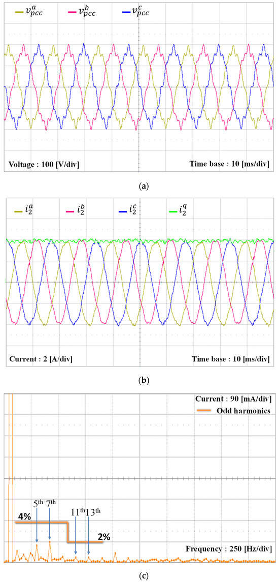
Figure 21.
Experimental results for the proposed scheme when uncertain LC-type grid impedance exists ( 3 mH and 8 µF). (a) Distorted PCC voltages; (b) Grid-side currents; (c) FFT result of a-phase grid-side current.
As the final test, the complex grid is set up with the grid inductance Lg of 3 mH and the grid capacitance increasing from 8 µF to 10 µF. Under such harsh conditions, the measured PCC voltages plotted in Figure 22a have a strong impact from the grid distortion. The FFT result of PCC voltage in Figure 22b clearly shows that the magnitudes of 7th and 11th harmonics highly increase up to 5% and 12.5% of the magnitude of the fundamental frequency. Even though the GCI system faces an extra grid dynamic caused by LC-type grid impedance, the proposed control scheme successfully stabilizes the entire GCI system with good quality currents, as in Figure 22c, because the complex grid condition is effectively taken into consideration in the controller design process. The robustness of the proposed scheme against LC-type grid impedance is well illustrated by the experimental results. The FFT result of the current in Figure 22d confirms that the 11th harmonic component in the PCC voltage of Figure 22b is well suppressed by the harmonic rejection of the proposed scheme by maintaining the distortion in the injected currents below the allowed limits.
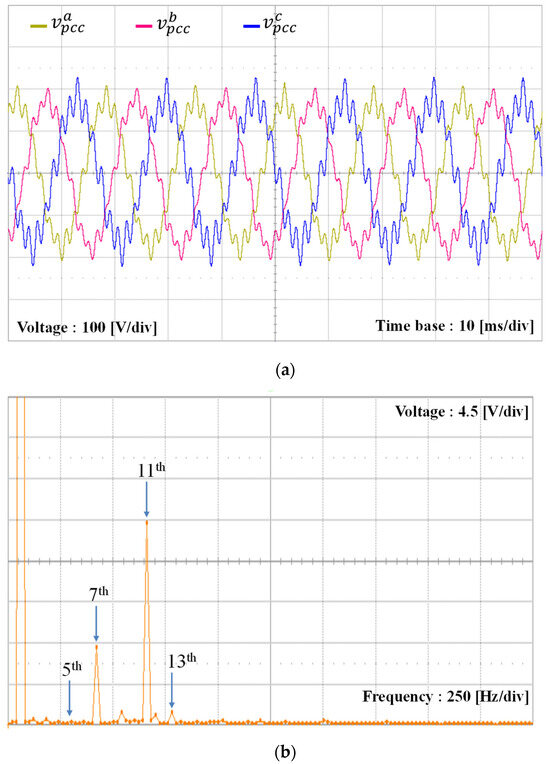
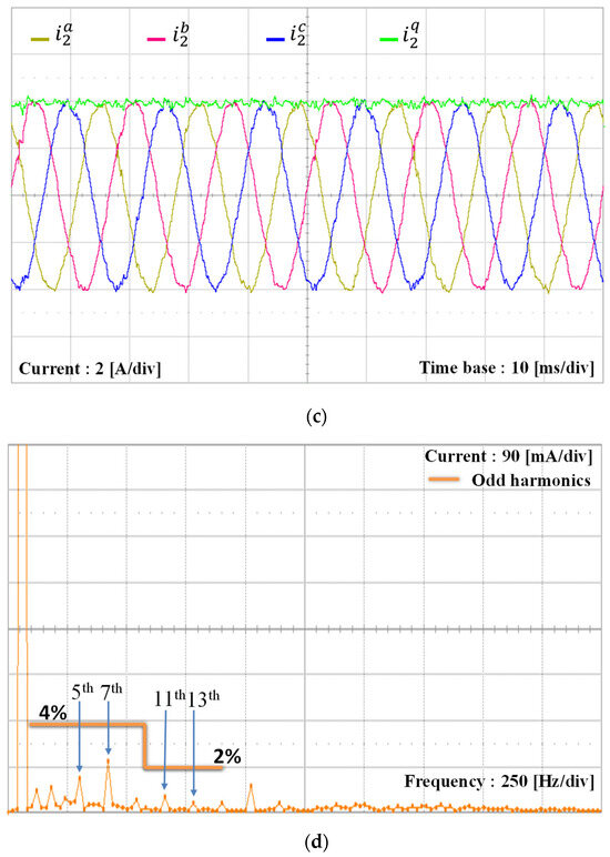
Figure 22.
Experimental results for the proposed scheme when uncertain LC-type grid impedance exists ( 3 mH and 10 µF). (a) Distorted PCC voltages; (b) FFT result of a-phase PCC voltage; (c) Grid-side currents; (d) FFT result of a-phase grid-side current.
6. Conclusions
In this paper, a current control scheme has been designed to stabilize an LCL-filtered GCI system under a distorted grid environment and uncertain grid impedance. First, to deal with the negative impact of grid impedance, LC-type grid impedance is considered in both the system model derivation and controller design process of an LCL-filtered GCI system. Moreover, the integral and resonant control components are also augmented into the system model to guarantee that the grid-injected currents from GCI will track the reference without influence by disturbance from a distorted grid. Next, an incomplete state feedback current controller based on the LQR has been developed to operate the GCI under grid impedances. The asymptotic stability, robustness, and resonance-damping capability of the proposed scheme have been confirmed by the closed-loop pole map evaluation even when all the system states are not available. Comprehensive evaluations have been conducted to validate the feasibility and effectiveness of the proposed control design when the LCL-filtered GCI is connected to an unexpected grid. All the simulation and experimental results have clearly proved that the proposed control scheme successfully stabilizes the entire GCI system with high-quality grid-injected currents even when the GCI faces severe grid distortions and an extra grid dynamic caused by the L-type or LC-type grid impedance.
Author Contributions
S.-D.K., T.V.T., S.-J.Y. and K.-H.K. conceived the main concept of the control structure and developed the entire system. S.-D.K. and T.V.T. carried out the research and analyzed the numerical data with guidance from K.-H.K., S.-D.K., T.V.T., S.-J.Y. and K.-H.K. collaborated in the preparation of the manuscript. All authors have read and agreed to the published version of the manuscript.
Funding
This study was supported by the Research Program funded by the SeoulTech (Seoul National University of Science and Technology).
Data Availability Statement
The original contributions presented in the study are included in the article, further inquiries can be directed to the corresponding author.
Conflicts of Interest
The authors declare no conflicts of interest.
Nomenclature
| Filter capacitance | |
| Grid capacitance | |
| Grid voltage vector | |
| Inverter-side current | |
| q-axis inverter-side current | |
| d-axis inverter-side current | |
| , | Grid-side current and reference current |
| , | q-axis grid-side current and reference current |
| , | d-axis grid-side current and reference current |
| Grid inductance current | |
| q-axis grid inductance current | |
| d-axis grid inductance current | |
| Optimal feedback control gain | |
| Incomplete state feedback control gain | |
| Observer gain | |
| Filter inductance | |
| Grid inductance | |
| Positive semi-definite matrix | |
| Positive definite matrix | |
| Reference current vector | |
| Sampling period | |
| System input vector | |
| One-step delay system input vector | |
| Capacitor voltage | |
| q-axis capacitor voltage | |
| d-axis capacitor voltage | |
| DC-link voltage | |
| Utility grid voltage | |
| q-axis utility grid voltage | |
| d-axis utility grid voltage | |
| Inverter output voltage | |
| q-axis inverter output voltage | |
| d-axis inverter output voltage | |
| PCC voltage | |
| q-axis PCC voltage | |
| d-axis PCC voltage | |
| System state vector | |
| Estimated state vector | |
| System output vector | |
| Integral and resonant terms vector | |
| Current error vector | |
| Gird phase angle | |
| Damping ratio | |
| Algular frequency of grid voltage |
References
- Yang, H.; Zhang, Y.; Liang, J.; Gao, J.; Walker, P.D.; Zhang, N. Sliding-mode observer based voltage-sensorless model predictive power control of PWM rectifier under unbalanced grid conditions. IEEE Trans. Ind. Electron. 2017, 65, 5550–5560. [Google Scholar] [CrossRef]
- Rodriguez-Diaz, E.; Freijedo, F.D.; Vasquez, J.C.; Guerrero, J.M. Analysis and comparison of notch filter and capacitor voltage feedforward active damping techniques for LCL grid-connected converters. IEEE Trans. Power Electron. 2018, 34, 3958–3972. [Google Scholar] [CrossRef]
- IEEE Std.1547; IEEE Standard for Interconnecting Distributed Resources with Electric Power Systems. IEEE: New York, NY, USA, 2003.
- Liserre, M.; Blaabjerg, F.; Hansen, S. Design and control of an LCL-filter-based three-phase active rectifier. IEEE Trans. Ind. Appl. 2005, 41, 1281–1291. [Google Scholar] [CrossRef]
- Pan, D.; Ruan, X.; Wang, X. Direct realization of digital differentiators in discrete domain for active damping of LCL-type grid-connected inverter. IEEE Trans. Power Electron. 2018, 33, 8461–8473. [Google Scholar] [CrossRef]
- Han, Y.; Yang, M.; Li, H.; Yang, P.; Xu, L.; Coelho, E.A.A.; Guerrero, J.M. Modeling and stability analysis of LCL-Type gridconnected inverters a comprehensive overview. IEEE Access 2019, 7, 114975–115001. [Google Scholar] [CrossRef]
- Li, X.; Wu, X.; Geng, Y.; Yuan, X.; Xia, C.; Zhang, X. Wide damping region for LCL-type grid-connected inverter with an improved capacitor-current-feedback method. IEEE Trans. Power Electron. 2014, 30, 5247–5259. [Google Scholar] [CrossRef]
- Wu, W.; Liu, Y.; He, Y.; Chung, H.S.H.; Liserre, M.; Blaabjerg, F. Damping methods for resonances caused by LCL-filter-based current-controlled grid-tied power inverters: An overview. IEEE Trans. Ind. Electron. 2017, 64, 7402–7413. [Google Scholar] [CrossRef]
- Me, S.P.; Zabihi, S.; Blaabjerg, F.; Bahrani, B. Adaptive virtual resistance for postfault oscillation damping in grid-forming inverters. IEEE Trans. Power Electron. 2022, 37, 3813–3824. [Google Scholar] [CrossRef]
- Kukkola, J.; Hinkkanen, M. Observer-based state-space current control for a three-phase grid-connected converter equipped with an LCL filter. IEEE Trans. Ind. Appl. 2014, 50, 2700–2709. [Google Scholar] [CrossRef]
- Kukkola, J.; Hinkkanen, M.; Zenger, K. Observer-based state-space current controller for a grid converter equipped with an LCL filter: Analytical method for direct discrete-time design. IEEE Trans. Ind. Appl. 2015, 51, 4079–4090. [Google Scholar] [CrossRef]
- Teodorescu, R.; Blaabjerg, F.; Liserre, M.; Loh, P.C. Proportional-resonant controllers and filters for grid-connected voltage-source converters. IEE Proc. Electr. Power Appl. 2006, 153, 750–762. [Google Scholar] [CrossRef]
- Liu, Y.; Wu, W.; He, Y.; Lin, Z.; Blaabjerg, F.; Chung, H.S.H. An efficient and robust hybrid damper for LCL or LLCL-based grid-tied inverter with strong grid-side harmonic voltage effect rejection. IEEE Trans. Ind. Electron. 2016, 63, 926–936. [Google Scholar] [CrossRef]
- Tran, T.V.; Yoon, S.-J.; Kim, K.-H. An LQR-based controller design for an LCL-filtered grid-connected inverter in discrete-time state-space under distorted grid environment. Energies 2018, 11, 2062. [Google Scholar] [CrossRef]
- Jia, Y.; Zhao, J.; Fu, X. Direct grid current control of LCL-filtered grid-connected inverter mitigating grid voltage disturbance. IEEE Trans. Power Electron. 2014, 29, 1532–1541. [Google Scholar]
- Liserre, M.; Teodorescu, R.; Blaabjerg, F. Stability of photovoltaic and wind turbine grid-connected inverters for a large set of grid impedance values. IEEE Trans. Power Election. 2006, 21, 263–272. [Google Scholar] [CrossRef]
- Parker, S.G.; McGrath, B.P.; Holmes, D.G. Regions of active damping control for LCL filters. IEEE Trans. Ind. Appl. 2014, 50, 424–432. [Google Scholar] [CrossRef]
- Chen, X.; Zhang, Y.; Wang, S.; Chen, J.; Gong, C. Impedance-phased dynamic control method for grid-connected inverters in a weak grid. IEEE Trans. Power Electron. 2017, 32, 274–283. [Google Scholar] [CrossRef]
- Huang, M.; Li, H.; Wu, W.; Blaabjerg, F. Observer-based sliding mode control to improve stability of three-phase LCL-filtered grid-connected VSIs. Energies 2019, 12, 1421. [Google Scholar] [CrossRef]
- Nam, N.N.; Nguyen, N.-D.; Yoon, C.; Lee, Y.I. Disturbance observer-based robust model predictive control for a voltage sensorless grid-connected inverter with an LCL filter. IEEE Access 2021, 9, 109793–109805. [Google Scholar] [CrossRef]
- Yoon, S.-J.; Kim, K.-H. Harmonic suppression and stability enhancement of a voltage sensorless current controller for a grid-connected inverter under weak grid. IEEE Access 2022, 10, 38575–38589. [Google Scholar] [CrossRef]
- Kim, Y.B.; Tran, T.V.; Kim, K.-H. LMI-based model predictive current control for an LCL-filtered grid-connected inverter under unexpected grid and system uncertainties. Electronics 2022, 11, 731. [Google Scholar] [CrossRef]
- Wang, J.; Yao, J.; Hu, H.; Xing, Y.; He, X.; Sun, K. Impedance-based stability analysis of single-phase inverter connected to weak grid with voltage feed-forward control. In Proceedings of the 2016 IEEE Applied Power Electronics Conference and Exposition (APEC), Long Beach, CA, USA, 20–24 March 2016; pp. 2182–2186. [Google Scholar]
- Qian, Q.; Xie, S.; Xu, J.; Ji, L. Harmonic suppression and stability improvement for aggregated current-controlled inverters. In Proceedings of the 2016 IEEE Energy Conversion Congress and Exposition (ECCE), Milwaukee, WI, USA, 18–22 September 2016; pp. 1–5. [Google Scholar]
- Harnefors, L.; Finger, R.; Wang, X.; Bai, H.; Blaabjerg, F. VSC input-admittance modeling and analysis above the Nyquist frequency for passivity-based stability assessment. IEEE Trans. Ind. Electron. 2017, 64, 6362–6370. [Google Scholar] [CrossRef]
- Wang, X.; Blaabjerg, F.; Loh, P.C. Passivity-based stability analysis and damping injection for multi-paralleled voltage-source converters with LCL filters. IEEE Trans. Power Electron. 2017, 32, 8922–8935. [Google Scholar] [CrossRef]
- Qian, Q.; Xu, J.; Ni, Z.; Zeng, B.; Zhang, Z.; Xie, S. Passivity-based output impedance shaping of LCL-filtered grid-connected inverters for suppressing harmonics and instabilities in complicated grid. In Proceedings of the 2017 IEEE Southern Power Electronics Conference (SPEC), Puerto Varas, Chile, 4–7 December 2017; pp. 1–6. [Google Scholar]
- Lichota, P.; Dul, F.; Karbowski, A. System identification and LQR controller design with incomplete state observation for aircraft trajectory tracking. Energies 2020, 13, 5354. [Google Scholar] [CrossRef]
- Franklin, G.F.; Powell, J.D.; Workman, M.L. Digital Control of Dynamic Systems; Addison-Wesley: Menlo Park, CA, USA, 1998; Volume 3. [Google Scholar]
- Patarroyo-Montenegro, J.F.; Vasquez-Plaza, J.D.; Andrade, F. A state-space model of an inverter-based microgrid for multivariable feedback control analysis and design. Energies 2020, 13, 3279. [Google Scholar] [CrossRef]
- Maccari, L.; Massing, J.; Schuch, L.; Rech, C.; Pinheiro, H.; Oliveira, R.; Montagner, V. LMI-based control for grid-connected converters with LCL filters under uncertain parameters. IEEE Trans. Power Electron. 2014, 29, 3776–3785. [Google Scholar] [CrossRef]
- Phillips, C.L.; Nagle, H.T. Digital Control System Analysis and Design, 3rd ed.; Prentice Hall: Englewood Cliffs, NJ, USA, 1995. [Google Scholar]
- Ogata, K. Discrete Time Control Systems, 2nd ed.; Prentice Hall: Englewood Cliffs, NJ, USA, 1995. [Google Scholar]

Disclaimer/Publisher’s Note: The statements, opinions and data contained in all publications are solely those of the individual author(s) and contributor(s) and not of MDPI and/or the editor(s). MDPI and/or the editor(s) disclaim responsibility for any injury to people or property resulting from any ideas, methods, instructions or products referred to in the content. |
© 2024 by the authors. Licensee MDPI, Basel, Switzerland. This article is an open access article distributed under the terms and conditions of the Creative Commons Attribution (CC BY) license (https://creativecommons.org/licenses/by/4.0/).