A Water-to-Water Heat Pump Model with Experimental Validation

Abstract

An experimental validation of a steady-state model for water-to-water heat pumps is conducted on a 10 kW test bench. The objective of the model is to predict the capacity and the required compressor power, based on the inlet conditions of the secondary fluids in the evaporator and condenser. Detailed manufacturer performance maps based on the AHRI 540-2020 standard are utilized to model the fixed-speed scroll compressor. A new semi-empirical model for the thermostatic expansion valve incorporates condensing temperature effects on superheating prediction. Sub-models for individual components, including detailed representations of the evaporator and condenser, are integrated into a global model, resulting in a set nonlinear equation solved using an equation solver with appropriate guess values. The validation of the model is conducted in an experimental test facility equipped with two precisely controlled secondary fluid loops. The heat pump is instrumented to measure condensation and evaporation pressures, the compressor discharge temperature, compressor power, superheating, and sub-cooling. The results are divided into three sub-sections: the first validates the complete heat pump model by comparing its power consumption and COPs in heating and cooling; the second compares the predicted and measured operational conditions; finally, it is shown how the model can be used to predict the non-operational conditions of the heat pump for specific scenarios.

1. Introduction

The development of accurate and reliable heat pump models can assist in enhancing the performance optimization of these systems and the overall efficiency of heating and cooling systems.

Most mechanical vapor compression heat pumps operate on a subcritical cycle below the critical point of the refrigerant. In their most basic configuration, heat is transferred from a source to a sink through a closed-loop refrigerant cycle, in four steps: evaporation, compression, condensation, and expansion [1]. In this article, water is used as the secondary fluid for both the source and sink. Water-to-water heat pumps are utilized in various applications, including ground-source heat pump (GSHP) systems [2].

This study aims to develop a validated experimental model for a water-to-water heat pump used to predict their overall performance as well as various critical parameters, including the thermodynamic states of the refrigerant at various cycle stages, their overall heat transfer coefficients, refrigerant flow rate, the discharge temperature from the compressor, and the degrees of superheat and sub-cooling. With the advent of various new refrigerants, such a detailed model can provide valuable and quick information on cycle performance. Unlike other modeling studies that fix one or several points in the refrigeration cycle, this study lets the model find the equilibrium state of the cycle based on the given inlet conditions (flow rate and temperature) of the water at the inlets of the evaporator and condenser. Additionally, the model identifies the non-operational states of the heat pump.

This paper is organized into five sections: The first section includes this short introduction. In the second section, the literature on water-to-water heat pumps is reviewed. This is followed, in the third section, by a presentation of the various sub-models used in the present study—a compressor, thermostatic expansion valve (TEV), and plate heat exchangers for the condenser and evaporator. The assembly of these sub-models into a comprehensive global model is also discussed. The experimental facility is presented in the fourth section, followed, in the last section, by a validation of the model and a presentation of its non-operational states.

2. Literature Review

Modeling heat pumps involves creating mathematical or computational representations to simulate and predict their performance under various conditions. Various methods exist for modeling heat pumps, which range in complexity. Analytical models, which utilize fundamental conservation laws of mass, energy, and momentum, are found on one end of the spectrum. These models also incorporate equations of state and basic heat transfer correlations to forecast the refrigerant’s state throughout the cycle. At the other end, there are models based solely on experimental data, which are either curve-fitted or arranged in performance maps. There are also semi-empirical models which lie in between these two extremes. The following literature review follows these categories by first presenting analytical approaches, and then empirical and semi-empirical models.

2.1. Analytical Models

Parise [3] developed a simulation model for vapor compression heat pumps to predict their overall system performance. This is accomplished by using a straightforward model for the components within the heat pump cycle. Input data, such as compressor speed, source and sink temperatures, and flow rates for the cooling and heating fluids, are entered to determine the system’s behavior. The condenser is regarded as having a constant overall heat transfer coefficient, which is determined based on its arithmetic overall temperature difference. A polytropic process is assumed to characterize the compression. Additionally, the superheat is assumed to be provided as an input.

Stefanuk et al. [4] introduced a steady-state model for a water-to-water heat pump operating with superheat control. This model is entirely based on fundamental conservation laws and key correlations of heat transfer, aimed at forecasting the heat pump’s performance across its entire operational range. The study’s results revealed that adjusting the refrigerant charge is an effective control mechanism to enhance system performance.

Herbas et al. [5] created a vapor compression model using straightforward mathematical representations for every component within the cycle. This approach resulted in a collection of nonlinear equations that were subsequently resolved using numerical techniques. Their model can predict the system’s operational conditions, including its condensation and evaporation pressures. A comparison between the model’s predictions and the performance of an existing unit showed a significant correlation. In the compressor model, a constant index polytropic process is presumed. It is assumed that the condenser maintains a constant overall heat transfer coefficient and the expansion valve is omitted from the model, given that the superheat levels are predetermined.

As part of a serious effort to evaluate the performance of potential alternative refrigerants, several cycle simulation models were developed by researchers from the National Institute of Standards and Technology (NIST). Initially, a cycle model named Cycle 7 was developed by McLinden [6], comprising seven cycle state points. Cycle 7 evolved by incorporating a suction-line heat exchanger and enhancements to the compressor model, leading to the emergence of Cycle 11 [7], which now encompasses eleven state points. The potential performance comparison of possible replacement refrigerants has been carried out using Cycle 11 [8,9]. Cycle 11 incorporates simplifications, including the absence of a pressure drop across heat exchangers, the utilization of polytropic compressor efficiency, constant degrees of superheat and sub-cooling, and fixed heat transfer coefficients in the heat exchangers.

Included within the models developed by the NIST is the Bicycle model [10], which serves the purpose of designing and evaluating the off-design performance of alternative refrigerant mixtures in vapor compression cycles. Among the primary assumptions employed are fixed degrees of superheating and sub-cooling. Fixed pressure drops across heat exchangers are also assumed, while the volumetric and isentropic efficiency of the compressor remain variable.

Since 1978, several versions of the DOE/ORNL Heat Pump Design Model (HPDM), which is a hardware-based steady-state performance simulation model, have been developed and disseminated by Oak Ridge National Laboratory (ORNL), as outlined by Rice [11]. The Mark V model has been released by ORNL [11].

Scarpa et al. [12] developed a thermodynamic-based heat pump model that relies on inputs such as compressor isentropic efficiency, heat exchanger effectiveness, and refrigerant flow rate. Its performance outcomes show up to 10% variances when compared to manufacturer data.

Ndiaye [13] created a dynamic model for a water-to-air heat pump to enhance the accuracy of its simulations. The investigation revealed that current models within energy simulation software fall short of accurately capturing the transient effects associated with cycling. It was observed that the time constant utilized for modeling the heat pump’s start-up capacity depends on its operating conditions, highlighting a weakness in the models used by simulation programs that rely on a fixed time constant. In a related study, Ndiaye and Bernier [14] developed a model predicting the state of the refrigerant throughout the circuit during typical operation and cycling conditions. The model can predict with relatively good accuracy the measured transient behavior of a GSHP. Similarly, to analyze the changes in energy consumption and capacity resulting from partial load operations and their associated shutdown and start-up processes, Ndiaye and Bernier [15] presented generalized one- and two-time-constant models.

IMST-ART (v4.10) is a software created for simulating refrigeration systems [16], with its applicability extending to heat pumps. The program offers multiple sub-models for compressors, heat exchangers, expansion valves, pipes, and accessories, allowing users to construct various refrigeration system configurations.

Dechesne et al. [17] investigated a residential air-to-water heat pump, specifically a split system that operates with a variable speed scroll compressor and utilizes R410A refrigerant. The system features an internal heat exchanger that evaporates the refrigerant injected into the scroll during compression. Their model employs five dimensionless polynomials to forecast compressor performance, although it lacks specifics on the heat exchanger’s design. The model inputs include the compressor’s rotational speed and the ratios of the total and injection pressures. Their findings underscore the positive effects of superheat control on heat pump efficiency, demonstrating that reducing suction superheat enhances both the coefficient of performance (COP) and heating capacity, while also lowering its discharge temperature.

Correa and Cuevas [18] introduced a model for an air-to-water heat pump aimed at residential space heating and domestic hot water. Their modular approach, similar to the one used in the present study, to modeling divides the heat pump into three components: a compressor, condenser, and evaporator. The model assumes constant evaporator superheat controlled by the expansion valve and condenser subcooling dictated by the refrigerant’s charge.

2.2. Experimentally Based Models

Experimentally based models prioritize simplicity and have the potential for high accuracy. With the growing availability of high-quality data from building energy metering and data-logging facilities, these models are expected to garner increasing attention [19]. They use statistical methods to establish the relationships between input parameters (e.g., ambient temperature, operating conditions) and the output performance of the heat pump (e.g., heating or cooling capacity, coefficient of performance). They are helpful when detailed theoretical equations are complex or when various system inefficiencies must be accounted for.

Gupta and Irving [20] established a correlation between heat pump performance and source/sink temperature difference using heat pump performance test results. When contrasted with the Building Research Establishment Domestic Energy Model (BREDEM) predictions, their resulting model exhibited an accurate reaction to variations in ambient temperature.

The validation of a black box heat pump model by Ruschenburg et al. [21] employed field monitoring results from five ground-source installations. Discrepancies ranging from 1% to 32% are observed for its coefficient of performance (COP). It was also determined that the influence of standby losses significantly affects its prediction of power consumption. Within the assessed installations, the standby period contributes to an electrical consumption ranging from 2% to 5%.

Nyika [22] developed a ‘black box’ model based on experimental data. Generic equipment models were created to capture the performance of families of similar heat pumps, which can be utilized in building simulation programs. Tabatabaei et al. [23] developed an empirical model specifically designed to ascertain the seasonal performance factor (SPF) of heat pumps directly. Their methodology encompasses six distinct approaches: four utilize polynomial functions, one employs an exponential function, and another uses the Carnot coefficient of performance (COP).

The TRNSYS software and its TESS library include some performance-map-based models, where heating (cooling) capacity and power consumption are given as a function of the source and load conditions. Actual performance is determined based on interpolation within the performance map. These models exhibit limitations, including diminished accuracy in their predictions of heat pump performance under part load conditions or when operating outside of the defined performance map. These shortcomings can be mitigated by integrating TRNSYS with additional software like the Engineering Equation Solver [24] and constructing a more comprehensive heat pump model, as Ghoubali et al. [25] suggested.

Bouheret and Bernier [26] presented the development of a model for a variable-capacity water-to-air ground-source heat pump. The model, designed for integration into TRNSYS, is constructed based on the manufacturer’s steady-state performance maps. It supports four operating modes: space heating, dedicated space cooling, simultaneous space cooling and domestic hot water (DHW) production, and dedicated (DHW) production. Controlled by a PI-type thermostat, the heat pump allows for the assessment of the required compressor frequency. In the study, the proposed model is employed in annual simulations of two residential buildings equipped with both variable-capacity and fixed-capacity heat pumps.

St-Onge et al. [27] presented a model of a variable-capacity air-source heat pump (VCASHP) in TRNSYS. By varying the heating loads and user-defined ambient temperatures, the impact of compressor frequency on the VCASHP’s performance was explicitly measured. The VCASHP model was constructed using multiple polynomial regressions. In contrast, the performance data released by manufacturers indicate that VCASHP can provide a significantly enhanced performance and capacity compared to single-speed machines; laboratory and field tests have revealed that its actual performance does not consistently align with these expectations.

Bordignon et al. [28] develop a streamlined model for simulating a ground heat exchanger and heat pump system. This model facilitates the estimation of energy usage and system efficiency in response to the operational conditions of its secondary fluids. Model parameters are calibrated using data from its operational performance or provided by manufacturers.

Woods and Bonnema [29] created a regression-based approach for modeling emerging heating, ventilation, and air-conditioning (HVAC) technologies, utilizing the user-defined coil object in the EnergyPlus building simulation software. The outputs from HVAC system models or experimental data can be employed to generate regression-based performance curves, which are subsequently utilized within building simulations. The regression approach is presented as an alternative to the direct modeling of new HVAC technologies in EnergyPlus.

2.3. Grey Box Models

A semi-empirical or grey box model is a mathematical model that combines both empirical data and theoretical principles to describe a system’s behavior and is used when a purely theoretical or entirely empirical model is inadequate to capture the system’s complexity or behavior accurately.

Underwood [30] developed a model with parameters that can be determined using manufacturer or experimental data. The compressor is at the heart of the model, characterized by exponential functions that incorporate four parameters. This model can forecast average test data values, exhibiting variations of up to 10% compared to experimental data. However, the model shows more significant discrepancies at elevated ambient temperatures.

Jin and Spitler [31] developed a steady-state simulation model for a reciprocating vapor-compression heat pump with a water-to-water configuration explicitly intended for incorporation into building simulation programs. This model is founded on basic thermodynamic principles and heat transfer relationships. It incorporates several undefined parameters, which are determined through a multi-variable optimization process using data provided by manufacturers.

Kinab [32] proposed a semi-empirical approach that relies on catalog data to establish their model parameters. This model features an isentropic compressor and employs polynomial laws to describe volumetric efficiency. Additionally, it accounts for the expansion valve and heat exchangers. This model can estimate the coefficient of performance (COP) of the heat pump within an accuracy of 8%.

Cimmino and Wetter [33] presented a Modelica model for simulating heat pumps. The model adopts a simplified vapor-compression cycle, encompassing only five refrigerant states. To determine the model’s parameters, an optimization procedure was employed, aiming to minimize the disparities between the model’s predicted heating capacities and power input and the corresponding values available in the manufacturer’s technical data. As a result of the calibration process, the heating capacities and power input calculated by the adjusted model were within a range of 2.7% and 4.7% of the manufacturer’s data, respectively.

Viviescas and Bernier [34] developed an exhaustive model for a variable-speed heat pump (VSHP) with a water-to-water configuration. The model is based on a physics-based methodology, integrating separate models for the plate heat exchangers (evaporator and condenser), the expansion valve, and the variable-speed compressor. The model requires five inputs: the mass flow rate and temperature of both secondary fluids and compressor speed. Furthermore, a performance map was constructed based on this comprehensive model. This performance map strategy yielded favorable outcomes for annual simulations compared to the entire model, showing maximum discrepancies of 2.5% in heating capacity and 5.1% in power consumption.

Advantages and disadvantages exist for physical models based on the refrigeration cycle and empirical models employing curve fitting [35]. In physical models, adaptation to operating conditions beyond the standard range is allowed, encompassing variations in refrigerant flow, superheating, sub-cooling, and other factors. However, in many cases, this adaptation comes at the expense of some precision in the model. On the other hand, models relying on curve fitting maintain good accuracy when their operating conditions fall within the data ranges used for curve fitting. In this case, extrapolation is somewhat undesirable.

From this review, it can be concluded that a comprehensive, detailed model of a water-to-water heat pump, which integrates each component individually and allows for the determination of the refrigerant’s energy performance and thermodynamic states, has not been found in the literature. More specifically, there does not appear to be many models that use the conditions of the secondary fluids (flow rate and inlet temperature) as input conditions. Furthermore, there is a notable absence of the experimental validation of such models.

3. Heat Pump Model

This model aims to predict the capacity (for either cooling or heating) and the necessary power of a heat pump based on predetermined inlet conditions for both secondary fluids (i.e., ${{T_w}_L}_{in}, {{\dot{m}}_w}_L, {{T_w}_S}_{in}, {{\dot{m}}_w}_S$ in Figure 1) without fixing cycle conditions such as its degrees of sub-cooling or superheating. This steady-state model also predicts the thermodynamic states of the refrigerant and the refrigerant flow rate (${\dot{m}}_r)$, the global heat exchange coefficients $\left(UA\right)$ of both heat exchangers, and the degrees of superheat (SH) and sub-cooling (SC) at the exits of the evaporator and condenser, respectively. Plate heat exchangers ($PHX$) are used in the evaporator and condenser. The heat pump features a fixed-speed scroll compressor, while a thermostatic expansion valve regulates the superheat level at the evaporator exit. 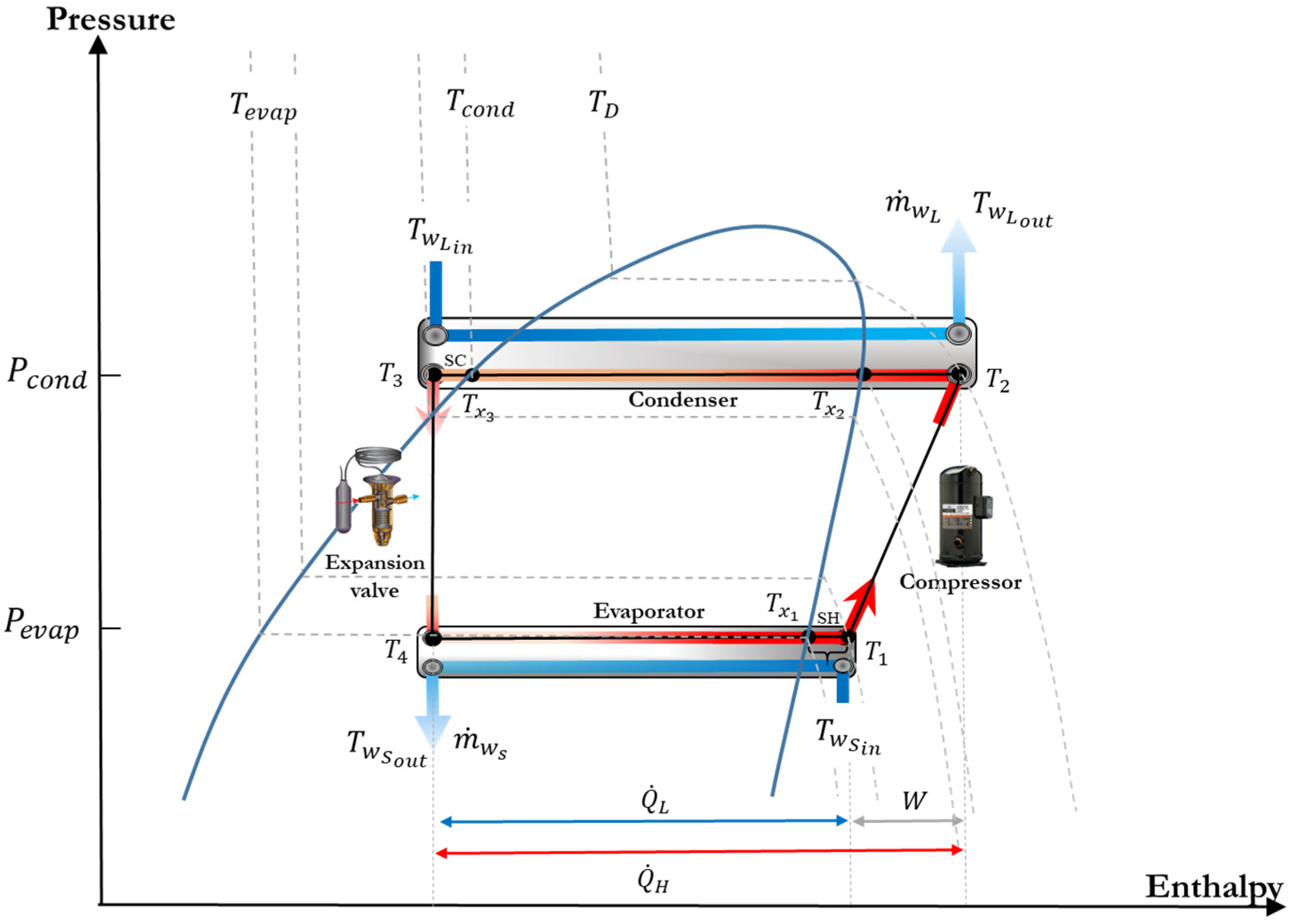Models for each component are interconnected through the refrigeration cycle depicted in Figure 1, in a classic pressure–enthalpy diagram. The reversing valve has been omitted for clarity. While the model developed here applies to residential-size heat pumps, it can be used for larger commercial heat pumps of similar designs.

The assumptions for each of the model components are listed in

Table 1. Assumptions used for the heat pump model and for all its components.

Component	Assumption
Evaporator and condenser	There are no pressure losses on the refrigerant side
	Heat losses between the exchangers and the surrounding environment are negligible
	Circulating oil has a negligible impact on heat transfer
Compressor	No heat losses between the compressor and the environment
Thermal expansion valve	Isenthalpic expansion process

. Steady-state conditions are assumed for all components.

In Figure 1, schematic overlays of the PHXs depict the heat transfer, involving secondary fluids at both the evaporator and condenser, when operating in heating mode. In cooling mode, ${{T_w}_L}_{in}$ and ${{T_w}_S}_{in}$ are reversed and represent the inlet secondary fluid temperatures to the evaporator and condenser, respectively. The refrigerant, R-410A in this instance, leaves the evaporator as a superheated vapor at the temperature $T_1$ and completes the compression process at ${ T}_2$. Within the condenser, the refrigerant undergoes an initial desuperheating from $T_2$ to $T_{x,2},$ condenses to a saturated liquid, and is further subcooled to $T_3$. Following this, an isenthalpic pressure reduction occurs in the expansion valve, leading to the refrigerant’s entry into the evaporator at $T_4$. Here, the refrigerant experiences evaporation from $T_4$ to $T_{x,1}$ and is subsequently superheated to ${ T}_1$.

3.1. Thermal Expansion Valve

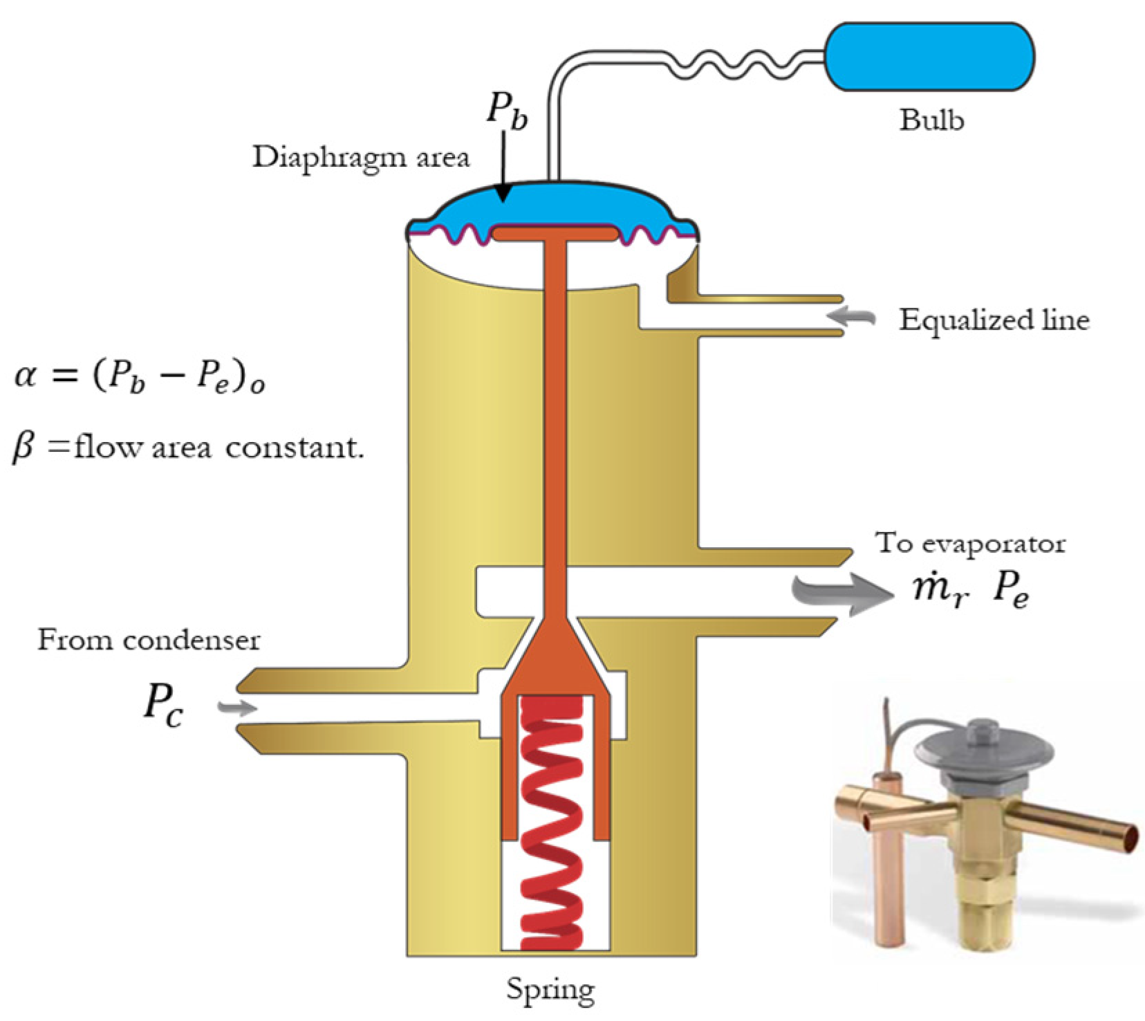
The modeled thermal expansion valve is depicted in Figure 2. The semi-empirical model used here is based on the work of Eames et al. [36] and is shown in Equation (1). It has the advantage of not requiring geometrical data to obtain the mass flow through the valve.

$${\dot{m}}_r=\beta \left[\left(P_b-P_e\right)-\alpha \right]\sqrt{2{\rho }_{rco}\left(P_c-P_e\right)} for \alpha \le \left(P_b-P_e\right)\le \delta$$

(1)

In Equation (1),${\dot{m}}_r$ is the mass flow rate of the refrigerant in kg/s, $\alpha$ is the pressure equivalent of the static superheat setting (SSS) (in kPa), $\delta$ is the value of $\left(P_b-P_e\right)$ when the valve is fully opened, $\beta$ is the constant flow area, $P_c$ and $P_e$ are the evaporator and condenser pressures (in kPa), $P_b$ represents the bulb pressure (in kPa), and ${\rho }_{rco}$ corresponds to the density of the refrigerant in its saturated liquid state in the condenser (in kg/m³).

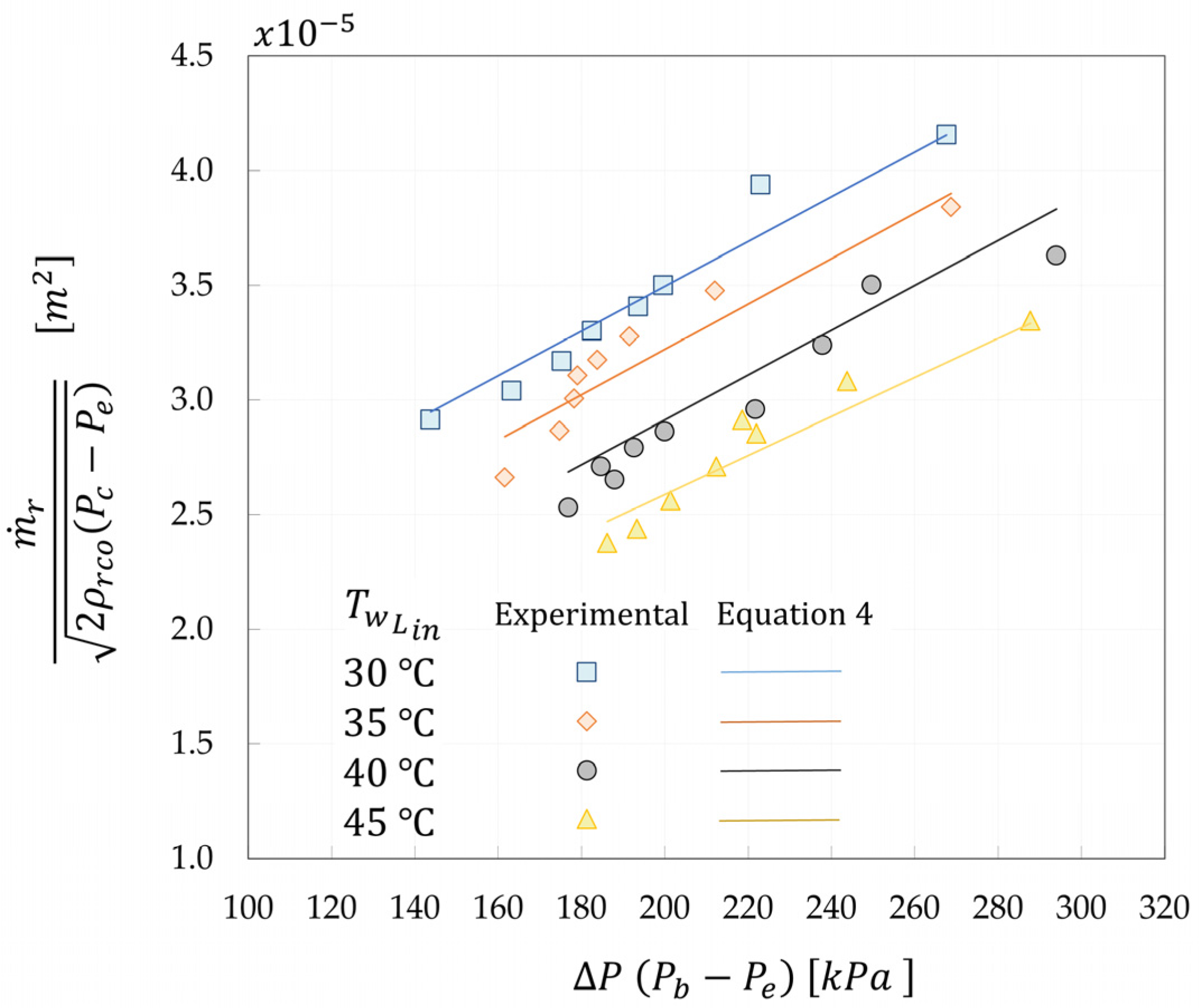
The values of $\alpha$ and $\beta$ are evaluated, using the linear regression curve of $\frac{{\dot{m}}_r}{\sqrt{2{\rho }_{rco}\left(P_c-P_e\right)}}$ against $\left(P_b-P_e\right)$, from the experimental data obtained with the test bench developed for the present study. These regressions are presented in Figure 3.

The evaporator and condenser pressures are measured using two pressure sensors with a $\pm$0.50% accuracy. The bulb pressure is calculated based on a temperature measurement made at the suction of the compressor. The refrigerant flow rate, ${\dot{m}}_r$, is calculated using the ten coefficients equation based on AHRI 540 [37], as a function of evaporating and condensing temperatures, as described later.

As observed in Figure 3, the lines depicting the refrigerant flow with a pressure drop between the compressor suction pressure ($P_b$) and the evaporating pressure ($P_e$) are influenced by the returning load fluid temperature (${T_w}_{L_{in}}$).

To establish a unified equation encompassing this influence, a modified version of Equation (1) is proposed:

$$\frac{{\dot{m}}_r}{\sqrt{{2\rho }_{rco}\left(P_c-P_e\right)}}=\beta \left[\left(P_b-P_e\right)-f\left({T_w}_L\right)\right]$$

(2)

where $f\left({T_w}_L\right)$ is represented as a function of $P_c,$ as shown in Equation (3).

$$f\left({T_w}_L\right)=f\left(P_c\right)=a{P}_c+b$$

(3)

By combining Equations (2) and (3), the final model used here is represented by Equation (4).

$$\frac{{\dot{m}}_r}{\sqrt{{2\rho }_{rco}\left(P_c-P_e\right)}}=\beta \left(P_b-P_e\right)-a{P}_c-b$$

(4)

The calibration of the coefficients a, b, and β is pivotal for the precise estimation of both the superheat temperature and the refrigerant’s mass flow rate. Using the experimental data and following a multivariable linear regression conducted using a popular statistical package, the model shows a multiple correlation coefficient R² of 0.94. Employing this model reveals a Root Mean Square Error (RMSE) of 1.9 × 10⁻³ kg/s and a maximum deviation of 7% in the prediction of the refrigerant’s mass flow rate.

3.2. Condenser and Evaporator Models

Various techniques can be employed to describe the heat exchange occurring in the condenser and evaporator. The lumped approach is frequently employed due to its simplicity. In this method, the whole heat exchanger is considered a single control volume, with an overall heat conductance value ($UA$) used to assess its efficiency. The performance of the heat exchanger is determined by employing either the logarithmic mean temperature difference (LMTD) method or the ε-NTU method to calculate its capacity.

The lumped approach is predominantly utilized when it is assumed that only one phase is present within the heat exchanger. However, when accounting for phase change transitions within the heat exchanger, a more elaborate model becomes necessary, such as the moving boundary modeling approach. In this model, which is used here, the heat exchanger is split into distinct zones, representing single-phase and two-phase regions, to accurately account for the complexities associated with phase change phenomena [38]. Following this, the governing equations in each zone are solved using a lumped approach. Initially, the total heat exchanger area distributions between each zone are undetermined and assigned initial guessed values. Then, an iterative procedure is employed, involving a set of nonlinear equations (comprising energy balances and epsilon-NTU equations within each zone) to ascertain the allocation of a heat exchanger area to each zone given the inlet conditions of the secondary fluids (flow rate and temperature).

The overall heat transfer coefficient ($U_i$) within each zone ($A_i)$ is essential for calculating the NTUs (Number of Transfer Units) value, as expressed in Equation (5).

$${NTU}_i=\frac{U_i{A}_i}{c_{min}}$$

(5)

This coefficient is computed based on the sum of three thermal resistances, as shown in Equation (6). In this equation, $h_{hot}$ and $h_{cold}$ are the convective heat transfer coefficients of the hot and cold sides, respectively, while $t_p \mathrm{and} k_p$ are the thickness and conductivity of the plate, respectively.

$$U=\frac{1}{\frac{1}{h_{hot}}+\frac{t_P}{k_P}+\frac{1}{h_{cold}}}$$

(6)

The term $t_p/k_p$ accounts for only about 1% of the overall heat transfer coefficient.

Due to the wide range of plate heat exchanger designs and flow regimes, different correlations are available for $h_{hot}$ and $h_{cold}$. Most of them are expressed based on the Nusselt number ($Nu$):

$$Nu=\frac{h{D}_h}{k}$$

(7)

where $D_h$ is the hydraulic diameter and $k$ is the fluid’s thermal conductivity. The hydraulic diameter is defined as

$$D_h=\frac{4A_x}{p}$$

(8)

where $A_x$ is the channel flow area, which is set equal to $bw$, where $b$ is the equivalent channel width, and $w$ is the plate heat exchanger width. The equivalent perimeter, denoted as p, is calculated as $p=2(b+\varphi w)$, where $\varphi$ is the surface enlargement factor. This is simplified to $p=2\varphi \mathrm{w}$, as b is significantly smaller than $w$ [39]. Thus, the hydraulic diameter is given by

$$D_h=\frac{4A_x}{p}=\frac{4bw}{2\varphi w}=\frac{2b}{\varphi }$$

(9)

3.2.1. Single-Phase Flows

For single-phase flows, heat transfer coefficients are obtained using the equations described by Wanniarachchi et al. [40] and Kim and Park [41]:

$$Nu={\left({{Nu}_t}^3+{{Nu}_l}^3\right)}^{\frac{1}{3}}{Pr}^{\frac{1}{3}}{\left(\raisebox{1ex}{${\mu }_b$}\!\left/ \!\raisebox{-1ex}{${\mu }_w$}\right.\right)}^{0.17}$$

(10)

$${Nu}_l=3.65{\varphi }^{0.661}{Re}^{0.339}/{\left(90-\beta \right)}^{0.455}$$

(11)

$${Nu}_t=12.6{\varphi }^{1-m}{Re}^m/{\left(90-\beta \right)}^{1.142}$$

(12)

$$m=0.646+0.0011\left(90-\beta \right)$$

(13)

$$Re=\frac{D_{h}V\rho }{\mu }=\frac{\dot{m}{D}_h}{N_{ch}wb\mu }$$

(14)

where $Re$ is the Reynolds number, $Pr$ is the Prandtl number, $\beta$ is the angle of the rib inclination angle of the plates (chevron angle), $\dot{m}$ represents the total mass flow rate, $N_{ch}$ indicates the number of channels for each fluid within the $PHX$, and $\mu$ is the dynamic viscosity of the fluid. These equations are valid on the refrigerant and water sides of the $PHX$.

3.2.2. Condensation

To calculate the heat transfer coefficient in the condensation mode, the equations proposed by Yan et al. [42] are used:

$$Nu=\frac{h{D}_h}{k_l}=4.118{{Re}_{eq}}^{0.4}{\mathrm{P}{\mathrm{r}}_l}^{1/3}$$

(15)

$${Re}_{eq}=\frac{G_{eq}{D}_h}{{\mu }_l}$$

(16)

$$G_{eq}=G\left[1-X_m+X_m\left(\frac{{\rho }_l}{{\rho }_v}\right)\right]$$

(17)

The equivalent Reynolds number (${Re}_{eq}$) is computed based on the equivalent mass flux ($G_{eq}$), while the mean vapor quality ($X_m$) represents the average vapor quality within the plate heat exchanger. The subscripts ‘$l$’ and ‘$v$’ signify properties associated with the saturated liquid and saturated vapor state.

3.2.3. Evaporation

In terms of the evaporation mode, Cascales et al. [43] noted that the model proposed by Cooper [44] closely aligns with experimental findings and this was consequently chosen for the current investigation. This model is represented by

$$\frac{h}{{\left(q/A\right)}^{0.67}}=55P_r^{\left[0.12-0.2{log}_{10}{R}_p\right]}{\left(-log{P}_r\right)}^{-55}{M}^{-0.5}$$

(18)

Here, $q/A$ is the heat flux rate, $M$ represents the molecular weight of the substance, and $P_r$ is the reduced pressure, defined as the operating pressure divided by the critical pressure of the fluid. The surface roughness parameter is denoted by $R_p$ (with a default value of $R_p=1$ when not explicitly specified, as is the case in the present study).

3.2.4. Condenser Heat Transfer Model

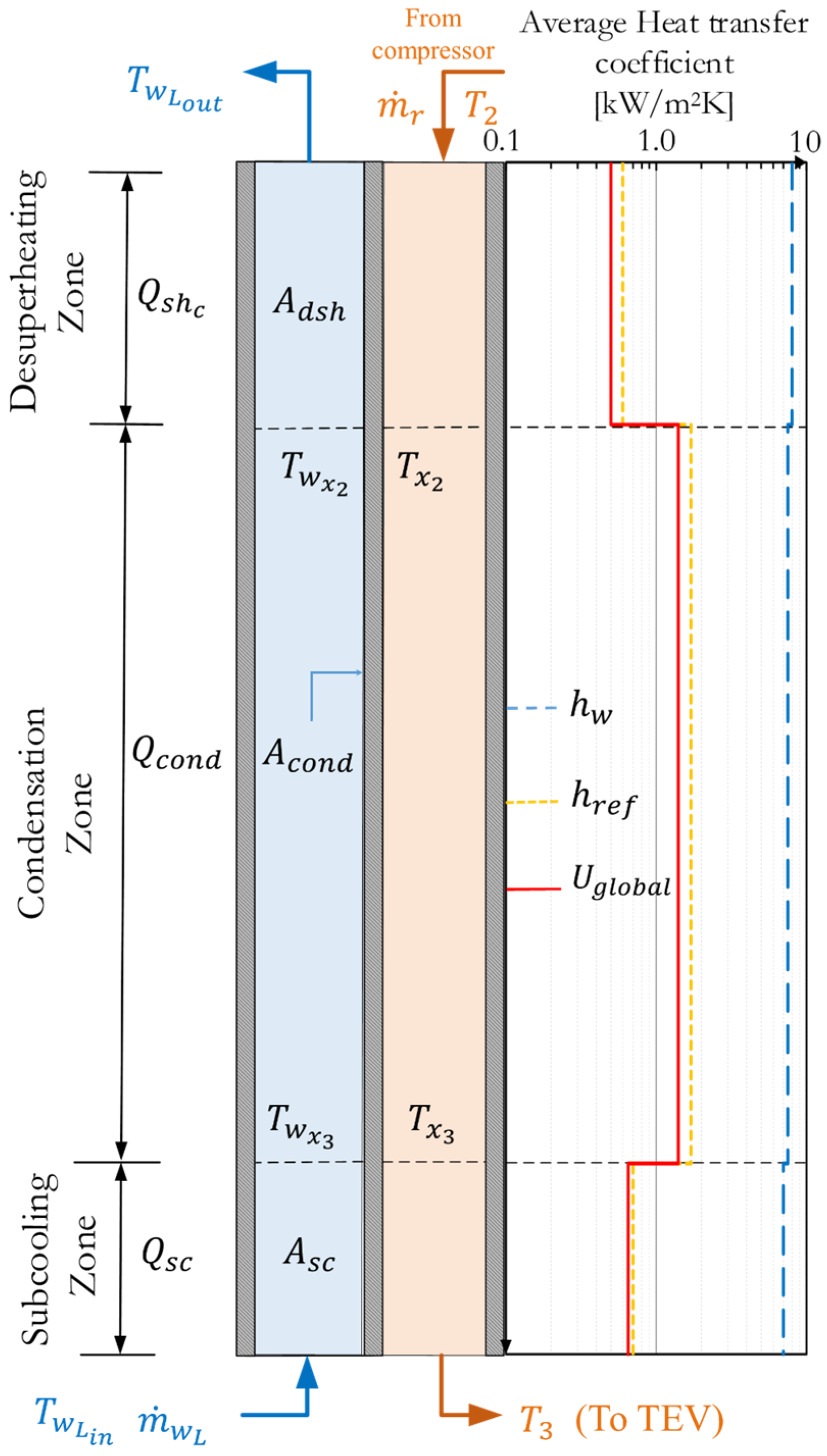
Figure 4 shows how the condenser’s counter-current flow is subdivided, with three distinct regions on the refrigeration side. The model can also simulate a parallel flow configuration, but this aspect of the model will not be presented here.

The total condenser heat transferred, $Q_{T_{cond}}$, equals the cumulative heat transfer in the desuperheating zone, $Q_{dsh}$, in the condensation zone,${ Q}_{cond}$, and in the subcooling zone,${ Q}_{sc}$.

$$Q_{T_{cond}}=Q_{dsh}+Q_{cond}+Q_{sc}$$

(19)

The total area for heat transfer is expressed as

$$A_{total}={(N}_c-1)A_p=A_{dsh}+A_{cond}+A_{sc}$$

(20)

The parameter $N_c$ represents the number of channels in the PHX. End plates, assumed to be adiabatic, are excluded from the total area calculation.

The heat transfer coefficients are significantly different in each section. Figure 4 provides an example of the average heat transfer coefficients on the water side ($h_w$) and on the refrigeration side ($h_{ref}$), as well as the overall coefficient $U_i$, for specific conditions: ${T_w}_{L_{in}}=35 °\mathrm{C}$, ${\dot{m}}_{w_L}=0.5 \mathrm{k}\mathrm{g}/\mathrm{s}$, $T_2=80 °\mathrm{C}$ and ${\dot{m}}_r=0.05 \mathrm{k}\mathrm{g}/\mathrm{s}$.

The blue dashed line represents the heat transfer coefficient for water, showing values ranging from $~$9 kW/m²-K in the superheating region to $~$7 kW/m²-K in the subcooling region. In contrast, the refrigerant (orange dashed line) displays coefficients of 0.6 kW/m²-K in the superheating zone, 0.8 kW/m²-K in the subcooling zone, and 1.8 kW/m²-K in the condensation zone. Consequently, the heat transfer process is predominantly controlled by the refrigerant side. As a result, the overall heat transfer coefficient (continuous red line) assumes values of $U_{sh}$ = 0.5 kW/m²-K in the superheating zone, $U_{cond}=$ 1.4 kW/m²-K in the condensation zone, and $U_{sc}=$ 0.7 kW/m²-K in the subcooling zone.

The plate heat exchanger model and the equations used in each heat exchanger zone are presented below. Thei thermophysical properties are evaluated at the mean temperature of the inlet and outlet conditions in each zone. All property calculations are performed using EES [24].

Desuperheating Zone

Equations (21)–(29) are the governing equations for this zone.

$$Q_{dsh}={\dot{m}}_r{C}_{p,r}\left(T_2-T_{x_2}\right)$$

(21)

$$Q_{dsh}={\epsilon }_{dsh}{c}_{min}\left(T_2-T_{w_{x_{2 }}}\right)$$

(22)

$$Q_{dsh}={\dot{m}}_w{C}_{p,w}\left(T_{w_{L_{out}}}-T_{w_{x2}}\right)$$

(23)

$$A_{dsh}=\frac{Q_{dsh}}{U_{dsh}{∆T}_{l{m}_{sh}}}=\frac{Q_{dsh}}{U_{dsh}\left[\left(T_2-T_{w_{L_{out}}}\right)-\left(T_{x_2}-T_{w_{x_{2 }}}\right)\right]}ln\frac{\left(T_2-T_{w_{L_{out}}}\right)}{\left(T_{x_2}-T_{w_{x_{2 }}}\right)}$$

(24)

$${\epsilon }_{dsh}=\frac{{1-e}^{\left[\left(-{NTU}_{dsh}\right)\left(1-C_r\right)\right]}}{1-C_r{e}^{\left[\left(-{NTU}_{dsh}\right)\left(1-C_r\right)\right]}}$$

(25)

$${NTU}_{dsh}=\frac{U_{dsh}{A}_{dsh}}{c_{min}}$$

(26)

$$C_r=\raisebox{1ex}{$c_{min}$}\!\left/ \!\raisebox{-1ex}{$c_{max}$}\right.$$

(27)

$$c_{max}=max({\dot{m}}_r{C}_{p,r}, {\dot{m}}_w{C}_{p,w})$$

(28)

$$c_{min}=min({\dot{m}}_r{C}_{p,r}, {\dot{m}}_w{C}_{p,w})$$

(29)

where $C_{p,w} \mathrm{a}\mathrm{n}\mathrm{d} C_{p,r}$ are the average heat capacities in the water and refrigerant zones, respectively.

Condensation Zone

Equations (30)–(34) model the condensation zone. The heat of condensation is determined by evaluating the enthalpy change during complete condensation, and this value is dependent on the condensation temperature ($T_{x_2}),$ as indicated in Equation (30).

$$Q_{cond}={\dot{m}}_r{∆H}_{evap\left(T_{x_2}\right)}$$

(30)

$$Q_{cond}={\epsilon }_{cond}{c}_{min}\left(T_{x_2}-T_{w_3}\right)$$

(31)

$$A_{cond}=\frac{Q_{cond}}{U_{cond}{∆T}_{l{m}_{cond}}}=\frac{Q_{cond}}{U_{cond}\left(T_{w_{x_{3 }}}-T_{w_{x_{2 }}}\right)}ln\left[\frac{\left(T_{x_2}-T_{w_{x_{2 }}}\right)}{\left(T_{x_2}-T_{w_{x_{3 }}}\right)}\right]$$

(32)

$${\epsilon }_{cond}=1-e\left(-{NTU}_{cond}\right)$$

(33)

$${NTU}_{cond}=\frac{U_{cond}{A}_{cond}}{c_{min}}$$

(34)

Subcooling Zone

In the subcooling zone, the governing equations are as follows:

$$Q_{sc}={\dot{m}}_r{C}_{p,r}\left({T_{x_2}-T}_3\right)$$

(35)

$$Q_{sc}={\dot{m}}_w{C}_{p,w}\left(T_{w_{x_{3 }}}-T_{w_{L_{in}}}\right)$$

(36)

$$Q_{sc}={\epsilon }_{sc}{c}_{min}\left(T_{x_3}-T_{w_{L_{in}}}\right)$$

(37)

$$A_{sc}=A_{total}-A_{cond}-A_{sh}$$

(38)

$${\epsilon }_{sc}=\frac{{1-e}^{\left[\left(-{NTU}_{sc}\right)\left(1-C_r\right)\right]}}{1-C_r{e}^{\left[\left(-{NTU}_{sc}\right)\left(1-C_r\right)\right]}}$$

(39)

$${NTU}_{sc}=\frac{U_{sc}{A}_{sc}}{c_{min}}$$

(40)

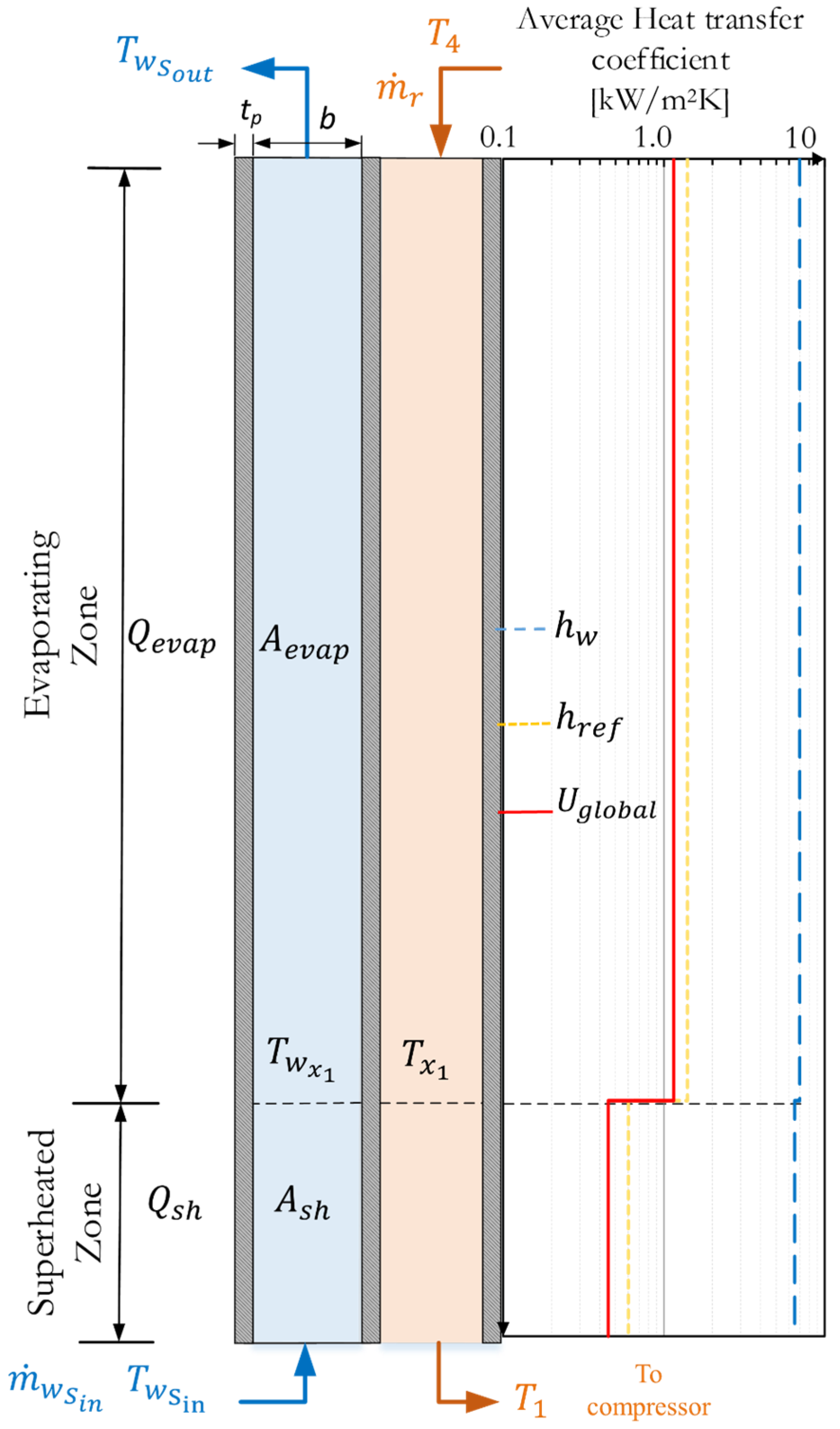
3.2.5. Evaporator Heat Transfer Model

The evaporator receives the refrigerant in the form of a vapor–liquid mixture after leaving the expansion valve. The heat transfer area in the plate heat exchanger is primarily utilized for the evaporation of the refrigerant until it reaches a saturated vapor state, and a smaller portion is used for superheating before being directed to the suction of the compressor. Figure 5 depicts the heat exchanges occurring between two adjacent plates of thickness $t_p$, where the water and the refrigerant flows are in opposite directions.

The total evaporator heat transfer $Q_{T_{evap}}$ is equal to the sum of the heat transferred in the evaporation zone, $Q_{evap}$, and the superheating zone, $Q_{sh}$ (Equation (41)).

$$Q_{T_{evap}}=Q_{sh}+Q_{evap}$$

(41)

The total area for heat transfer is expressed as

$$A_{tota{l}_{evap}}={(N}_c-1)A_p=A_{\mathrm{s}\mathrm{h}}+A_{evap}$$

(42)

Figure 5 provides an overview of the general variations of each heat transfer coefficient, as well as the overall coefficient $U_i$ for the specific conditions: ${T_w}_{s_{in}}=10 °\mathrm{C}$ ${\dot{m}}_{w_L}=0.5 \mathrm{k}\mathrm{g}/\mathrm{s}$, $T_4=5 °\mathrm{C}$, and ${\dot{m}}_r=0.05 \mathrm{k}\mathrm{g}/\mathrm{s}$.

The blue dashed line represents the heat transfer coefficient for water, which has values ranging from 7 kW/m²-K in the superheating region to 6 kW/m²-K in the evaporating region. In contrast, the refrigerant (orange dashed line) displays coefficients of 0.6 kW/m²-K in the superheating zone and 1.3 kW/m²-K in the evaporating zone. Consequently, as was the case for the condenser, the refrigerant side predominantly controls the heat transfer process. As a result, the overall heat transfer coefficient (continuous red line) assumes values of $U_{sh}$ = 0.5 kW/m²-K in the superheating zone and $U_{evap}=$ 1.1 kW/m²-K in the evaporating zone.

Evaporation Zone

Equations (43)–(47) are the governing equations for the evaporation zone.

$$Q_{evap}={\epsilon }_{evap}{c}_{min}\left(T_{w_{x1}}-T_{x_1}\right)$$

(43)

$${\epsilon }_{evap}=1-e\left(-{NTU}_{evap}\right)$$

(44)

$${NTU}_{evap}=\frac{U_{evap}{A}_{evap}}{c_{min}}$$

(45)

$$Q_{evap}={\dot{m}}_w{C}_{p,w}\left(T_{w_{x_1}}-T_{w_{S_{out}}}\right)$$

(46)

$$Q_{evap}={\dot{m}}_r{(1-x_4)∆H}_{evap}={\dot{m}}_r\left(1-x_4\right)f\left(T_{x_1}\right)$$

(47)

Superheating Zone

In this zone, the heat transfer is governed by the following equations:

$$Q_{sh}={\dot{m}}_r{C}_{p,r}\left(T_1-T_{x_1}\right)={\dot{m}}_r{C}_{p,r}∆T_{sh}$$

(48)

$$Q_{sh}={\dot{m}}_w{C}_{p,w}\left(T_{w_{S_{in}}}-T_{w_{x_1}}\right)$$

(49)

$${\mathrm{A}}_{sh}=\frac{Q_{sh}}{U_{sh}{∆T}_{l{m}_{sh}}}$$

(50)

3.3. Compressor Model

Various approaches to modelling compressors have been proposed. The Winandy model [45] is a semi-empirical gray box model designed to forecast scroll compressor performance. This model has been used as a basis for developing similar models such as those of Meramveliotakis [46]. Other semi-empirical models have been presented by Tello [47], Popovic and Shapiro [48], Klein [49], Li [50], and Shao et al. [51].

While most models typically assume a steady state, Ndiaye and Bernier [52] introduced a dynamic model for a hermetic reciprocating compressor operating across on–off cycles in their heat pump model. There is good agreement between this model and experiments conducted under steady-state and transient conditions in both heating and cooling scenarios.

In a recent investigation carried out by Gabel and Bradshaw [53], it was determined that the AHRI model, which features ten coefficients, demonstrates outstanding performance when trained with datasets encompassing both standard and variable superheat scenarios, revealing slight variances of 0.43% and 0.57% for mass flow rate and power, respectively. When compared against the models of Shao et al. [51], Popovic and Shapiro [48], and Winandy et al. [45], Aute et al. [54], also reported similar findings regarding the performance of the AHRI model [37] when trained with data.

Considering these conclusive studies, the AHRI model is used in this work. As shown in Equation (51), the AHRI model consists of a third-order polynomial equation with ten coefficients.

$$X=C_1+C_2{T}_S+C_3{T}_D+C_4{T}_S^2+C_5{T}_D{T}_S+C_6{T}_D^2+C_7{T}_S^3+C_8{T}_D{T}_S^2+C_9{T}_S{T}_D^2+C_{10}{T}_D^3$$

(51)

Here, $X$ represents the power input or the refrigerant mass flow rate, while $C_1$ to $C_{10}$ denote the regression coefficients supplied by the manufacturer, $T_D$ stands for the discharge dew-point temperature ($T_{x,2}$ in Figure 1), and $T_S$ is the suction dew-point temperature ($T_{x,1}$ in Figure 1). Manufacturers typically provide the coefficients for default units specified in °F for temperature, lb/h for mass flow rates, and watts for power.

The coefficients in Equation (51) are based on a specific value for the degrees of superheat, typically set at 5 °C. According to the AHRI 540 standard [37] changes in the degrees of superheat have no impact on compressor power; however, an adjustment in the mass flow rate is necessary. For this purpose, Equation (52) in Appendix D of the AHRI standard [37], is used to adjust the rated refrigerant mass flow rate, ${\dot{m}}_{rated}$, for the rated superheat to derive the corrected mass flow rate, ${\dot{m}}_{corrected}$, under the actual suction conditions.

$${\dot{m}}_{corrected}=\left\{1+F_V\left[\left(\frac{{\nu }_{rated}}{{\nu }_{corrected}}\right)-1\right]\right\}{\dot{m}}_{rated}$$

(52)

Within this equation, $F_V$ represents the correction factor for volumetric efficiency, which fluctuates according to the volumetric efficiency associated with the compression technology. The standard recommends using a value of one (1) as a general approximation. The additional variables in Equation (52) include ${\nu }_{corrected}$, the specific volume under the suction condition, and $v_{rated}$, the specific volume under the rated condition.

Predicting compressor performance following the AHRI 540 model presents two principal sources of uncertainty: the measurement and regression uncertainties encountered during model development. While the literature has quantified measurement uncertainty, the regression uncertainty may lead to average errors of up to 5% and 4% in power and mass flow rate predictions, respectively, as demonstrated in the studies conducted under AHRI-Project-8013 [54], and by Aute and Martin [55]. A technique for quantifying the uncertainty in the compressor map’s output was introduced by Cheung et al. [56], where the most important source of uncertainty is due to data training.

3.4. Numerical Solution

A set of equations representing the heat pump under study has been described. They include the compressor (governed by the power and mass flow rates in Equation (51)) and two heat exchangers (described by the heat exchange Equations (19)–(50)) as well as the heat transfer model (outlined through Equations (5)–(18)), the expansion device (specified by Equation (4)), and ultimately an equation of state to determine thermodynamic variables and physical properties of the system. A converged solution to this set of equations presents challenges, and two approaches are generally employed [57]. First, a non-simultaneous, component-based successive approach, where each variable or component of the heat pump is individually resolved to convergence before addressing the next unknown variable or component. The second approach, which is used in the present study, solves the set of equations simultaneously. A multi-variable nonlinear equation solver [24], is used to obtain the unknown variables within the convergence criteria which is set at 10⁻⁶ in the present case. However, the primary challenge when solving this system of equations lies in selecting initial guess values. No general rule can be established for the selection of guess values. Their selection relies on the experience of the modeler.

4. Experimental Test Facility

The heat pump under test is a commercially-available 3-Ton (10 kW) machine equipped with a scroll compressor. The set of ten coefficients for this compressor is presented in

Table 2. Input coefficients for Equation (51) for the compressor.

	Power [W]	Mass Flow Rate [lb/h]
C1	−561.362	250.7
C2	−15.626	5.011
C3	46.925	−1.456
C4	−0.2179	0.0409
C5	0.4351	−0.0178
C6	−0.4424	0.0171
C7	0.00022	0.00005
C8	0.00237	−5.09 × 10−6
C9	−0.00332	0.000147
C10	0.00250	−9.63 × 10−5

and is valid for a superheat of 5 °C.

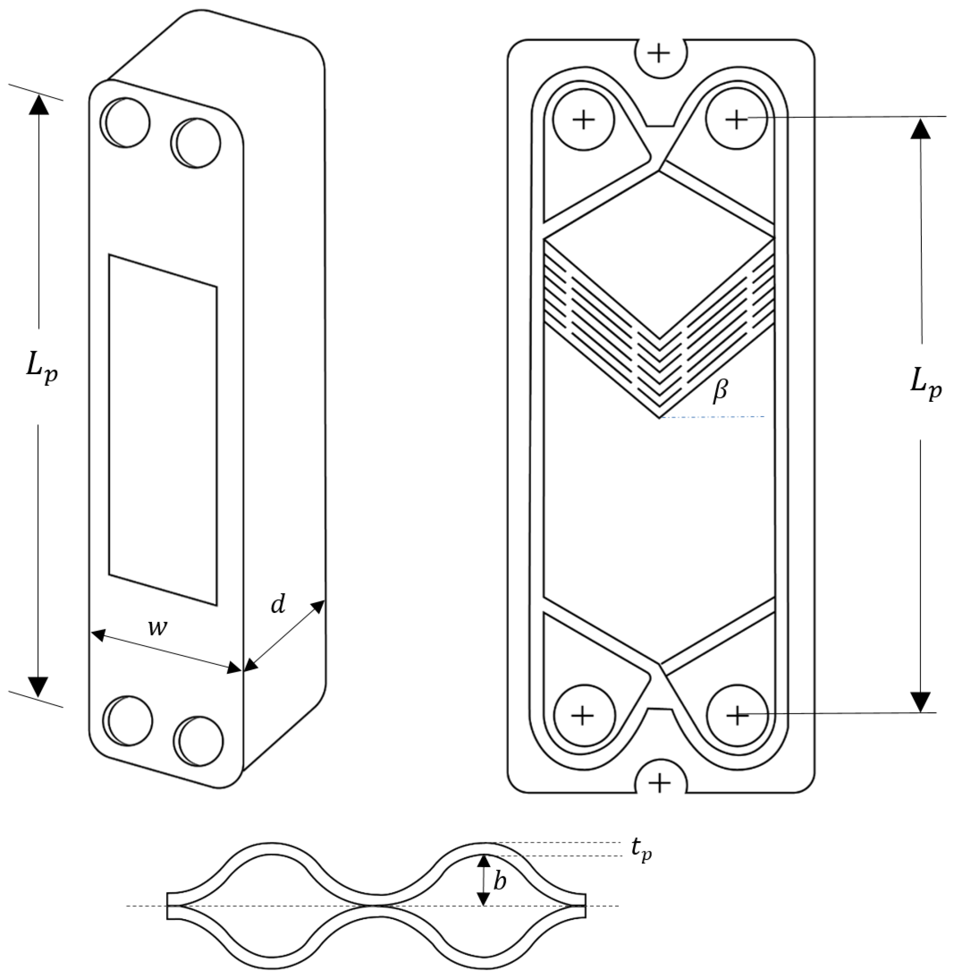
Two (2) SWEP P80 series brazed plate heat exchangers are used as the evaporator and the condenser. The main characteristics of these plate heat exchangers are presented in Figure 6 and

Table 3. Plate heat exchanger characteristics.

Parameter	Value	Units
$\mathrm{Width}\times$ height	$119 \times$ 526	$\mathrm{mm}\times$ mm
Depth of the condenser	122	mm
Depth of the evaporator	99	mm
Chevron angle, β	45	⃘
$\mathrm{Plate} \mathrm{thickness}, {\mathit{t}}_{\mathit{p}}$	0.8	mm
Plate spacing, b	1.7	mm
Surface enlargement factor, $\varphi$	1.2	-
$\mathrm{Hydraulic} \mathrm{diameter}, {\mathit{D}}_{\mathit{h}}$$(=2b/\varphi$)	2.8	mm
$\mathrm{Effective} \mathrm{surface} \mathrm{area}, A_p$	0.07	m2/plaque
Number of plates in the evaporator	40	-
Number of plates in the condenser	50	-
$\mathrm{Plate}’\mathrm{s} \mathrm{refrigerant}-\mathrm{side} \mathrm{thermal} \mathrm{conductivity} \left(\mathrm{Cooper}\right), {{\mathrm{k}}_{\mathrm{p}}}_r$	380	W/m-K

. They are based on information either provided or calculated based on the manufacturer’s data.

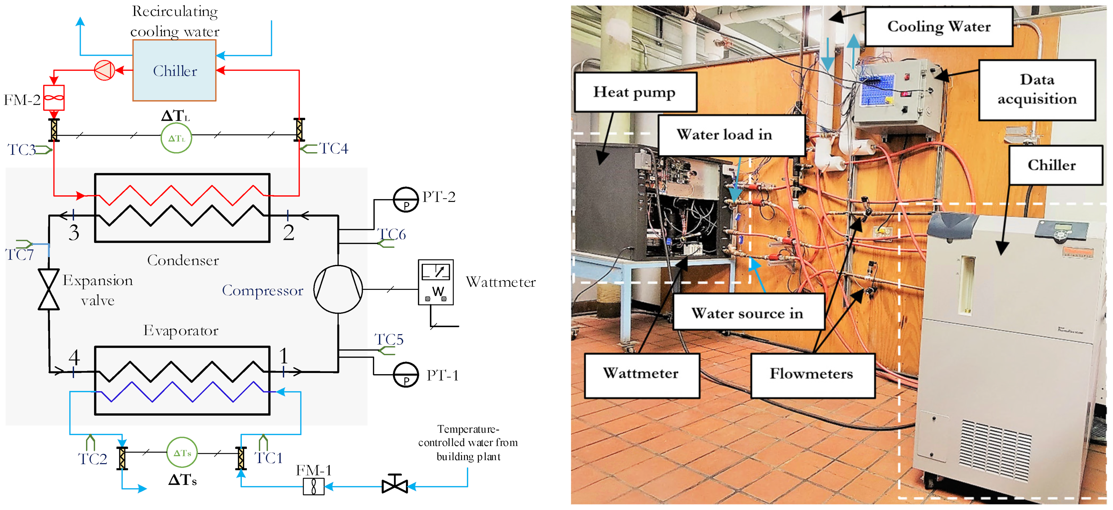
A schematic representation and a photograph of the experimental test facility are shown in Figure 7, and the main elements are presented in

Table 4. Instrumentation used in the test facility.

Measurement	Manufacturer	Uncertainty	Range
Flowmeter (${\dot{m}}_{w,l}$ and ${\dot{m}}_{w,s}$)	Omega (Norwalk, CT, USA) 1″ Turbine Flow Meter, 35 GPM (up to 2.2 L/s)	±0.5% of measurement	0.06–2.2 (L/s)
Wattmeter (W)	Ohio Semitronics (Hilliard, OH, USA) #WT3-12-100-D	±0.5% of full scale	0–24 [kW]
Differential temperature ($∆T_l$ and $∆T_s$)	Delta T Company (Pico Rivera, CA, USA) Thermopile, 20 junctions with Type T thermocouples	±0.04 [K]	0–140 [°C]
Pressure transducer (PT1, PT2)	Omega 1000 PSIG PX119 (Norwalk, CT, USA) Pressure transducer	±0.5% of measurement	0 to 7000 kPa
Temperature (TC1 to TC7)	Omega (Norwalk, CT, USA) Type T thermocouples	±0.1 [K]	0–200 [°C]

. The test bench comprises two precisely controlled secondary fluid loops and the heat pump under test. The heat pump is instrumented to measure condensation and evaporation pressures, the discharge temperature of the compressor, compressor power, degrees of superheating, and degrees of sub-cooling.

In heating mode, the condenser is connected to a water-cooled 10 kW recirculating chiller equipped with an electric heater to control and maintain the inlet temperature of the secondary fluid, with a stability of $\pm$0.1 °C. The chiller has a pump capable of delivering a flow rate of up to 0.63 L/s with a stability of $\pm$0.002 L/s. The evaporator is connected to a recirculating temperature-controlled water source available within the building, which provides water at stable temperatures ($\pm 0.1°\mathrm{C})$ and flow rates ($\pm$0.003 L/s).

The total heat exchanged in the evaporator and condenser is determined using Equations (53) and (54).

$${\dot{Q}}_L={\dot{m}}_{w,l}{C}_{p,l}∆T_l$$

(53)

$${\dot{Q}}_S={\dot{m}}_{w,s}{C}_{p,s}∆T_s$$

(54)

where $∆T_l$ and $∆T_s$ are the temperature differences of the secondary fluids across the heat exchangers. Given the significance of precisely measuring these temperature differences, two thermopiles have been incorporated into each of the secondary fluids’ circuits. Both have a measurement uncertainty of ±0.04 K in terms of the temperature difference, as indicated in Table 4. The specific heat of both secondary fluids (water),$C_{p,l}$ and $C_{p,s}$, is evaluated at the mean fluid temperature.

The mass flow rate is measured using a turbine-type flowmeter, the temperature is monitored using thermocouples, and the power is determined using a power meter. Details of the instruments used are outlined in Table 4. Sensors are connected to the data acquisition system.

The uncertainty of the measured $COPs$ and capacities reported later are calculated using the propagation of uncertainty technique presented by Taylor and Kuyatt [58], and based on the individual measurement uncertainties reported in Table 4.

A total of 32 experiments are reported in the heating mode, with eight different source temperatures (${T_w}_{S_{in}})$, ranging from 10 °C to 26 °C in increments of 2 °C, and four load temperatures (${T_w}_{L_{in}})$, ranging from 30 to 45 °C in increments of 5 °C. For the cooling mode, a series of 12 experiments are reported, with three temperatures for the load (10, 12, and 15 °C) and four temperatures for the source (27, 30, 35, and 40 °C). The mass flow rate of the secondary fluids is set at 0.565 L/s for the load and in the range of 0.308–0.462 L/s for the source side.

A typical experiment would proceed as follows: the temperature and flow rates are monitored until they reach a steady state, typically taking about 10 min. This 10 min period is carefully monitored so as to avoid slowly evolving drifts. Then, readings are taken every 0.1 s. for 30 s. The resulting 300 readings are then averaged and represent one data point.

5. Results

This results section is divided into three sub-sections. The validation of the complete heat pump model is presented first. This involves the comparison of its COPs and power consumption in both heating and cooling modes. The objective of this validation is to compare the modeling and experimental results for the same set of inlet conditions for both secondary fluids (i.e., ${{T_w}_L}_{in}, {{\dot{m}}_w}_L, {{T_w}_S}_{in}, {{\dot{m}}_w}_S)$. The second sub-section compares the operational conditions (evaporating and condensing temperatures, degrees of superheat and sub-cooling, and compressor discharge temperature) predicted by the model and those measured experimentally. Finally, it is shown how the model can be used to predict the non-operational conditions of the heat pump in specific scenarios.

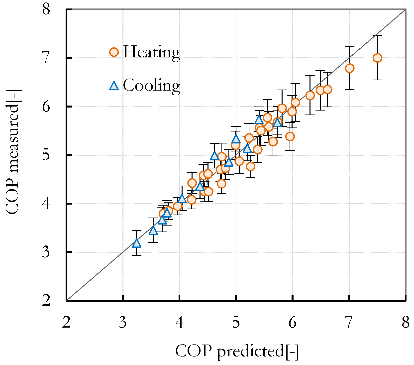
5.1. Coefficient of Performance (COP)

The coefficient of performance (COP) is defined as the ratio of the useful heating or cooling output to the power input required to achieve that output. Given the terminology used in Figure 1, the heating and cooling COP can be expressed as

$$CO{P}_H=\frac{{\dot{Q}}_H}{W}$$

(55)

$$CO{P}_C=\frac{{\dot{Q}}_L}{W}$$

(56)

As depicted in Figure 8, there is excellent agreement between the modeling results and experimental data in both the heating and cooling modes. When accounting for uncertainty, most data points closely align with the 45° line, representing perfect agreement.

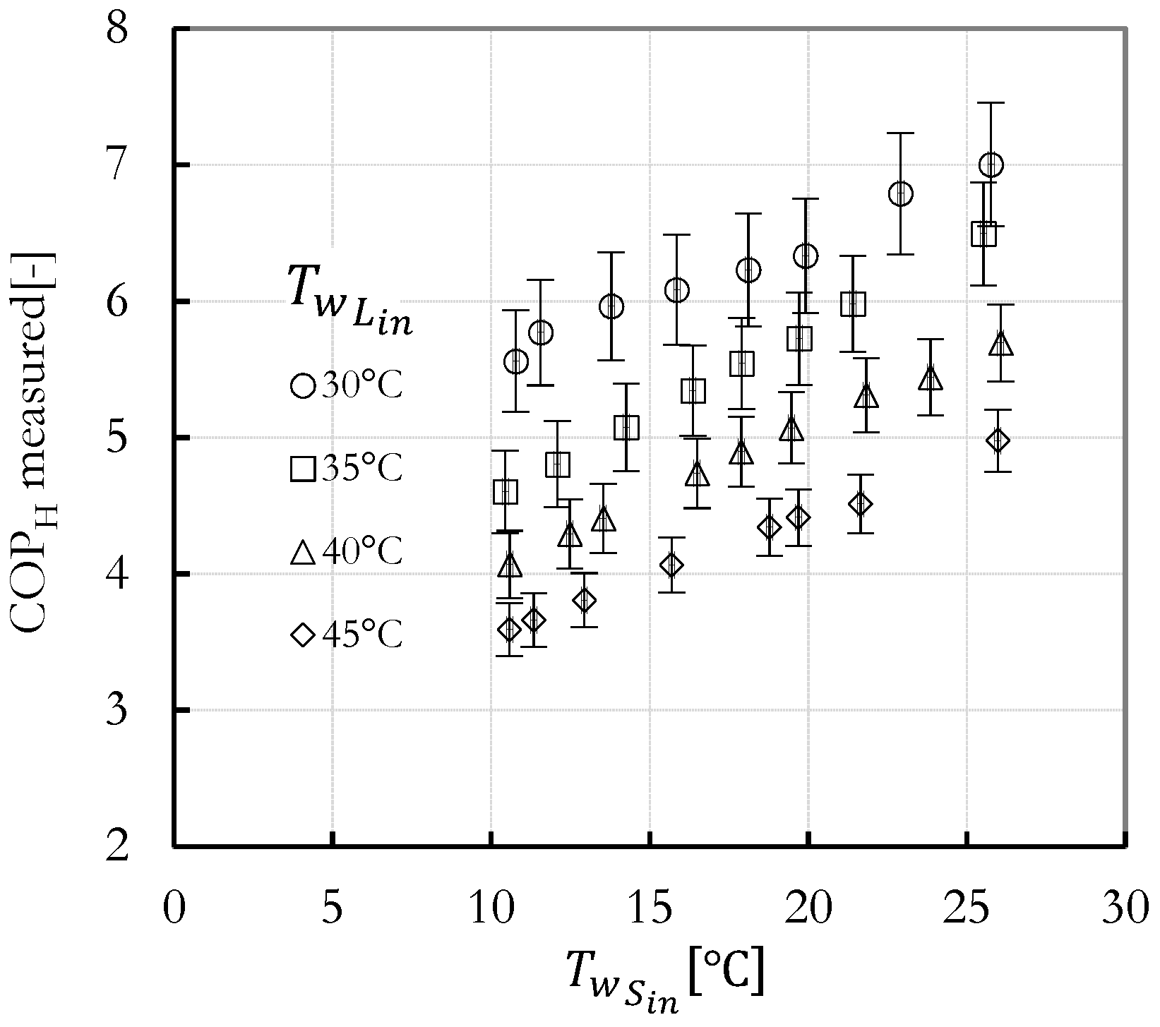
Figure 9 displays the $CO{P}_H$ across eight values of $T_{{w_S}_{in}}$ and four variations of $T_{{w_L}_{in}}$. As anticipated, the $CO{P}_H$ rises when the temperature difference between the source and load decreases. It increases by a factor of two (from $~$3.5 to $~$7) when the pair ($T_{{w_S}_{in}},$ $T_{{w_L}_{in}})$ changes from (10, 45 °C) to (20, 30 °C). Additionally, the $CO{P}_H$ increases when the $T_{{w_S}_{in}}$ increases for a given value of $T_{{w_L}_{in}}$.

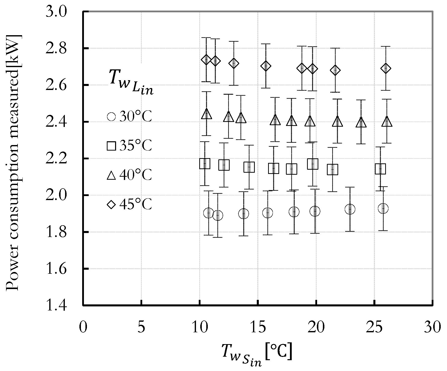
Figure 10 illustrates the measured power consumption as a function of the inlet temperatures of the secondary fluids, $T_{{w_L}_{in}}$ and $T_{{w_S}_{in}}$. An increase in the difference between these two temperatures leads to an increase in power consumption. However, for a given value of $T_{{w_L}_{in}},$ the source inlet temperature, $T_{{w_S}_{in}}$, has a relatively minor impact on power consumption. This is due to two competing effects. First, recall that the required compressor power is given by ${\dot{m}}_r\left(h_2-h_1\right)$, where $h_2$ represent the enthalpy of the refrigerant, which is associated with the discharge temperature $T_2$, and $h_1$ is the enthalpy associated with the suction temperature $T_1$ (Figure 1). A rise in suction temperature $T_1$, induced by an increase in $T_{{w_S}_{in}}$, results in increased density, attributed to the rise in evaporation pressure. There is also a slight increase in the degrees of superheat, which decreases density. However, the increase caused by the rise in the evaporation pressure is much greater. An increase in refrigerant density at the suction of the compressor leads to an increase in the mass flow rate, ${\dot{m}}_r$. In turn, this increase in mass flow rate contributes to a decrease in the compressor’s discharge temperature when operating under a constant condenser pressure, leading to a reduction in enthalpy change $\left(h_2-h_1\right)$. In the end, these effects cancel each other out, leaving the required compressor power almost unaffected by $T_{{w_S}_{in}}$.

5.2. Comparison of Operational Conditions

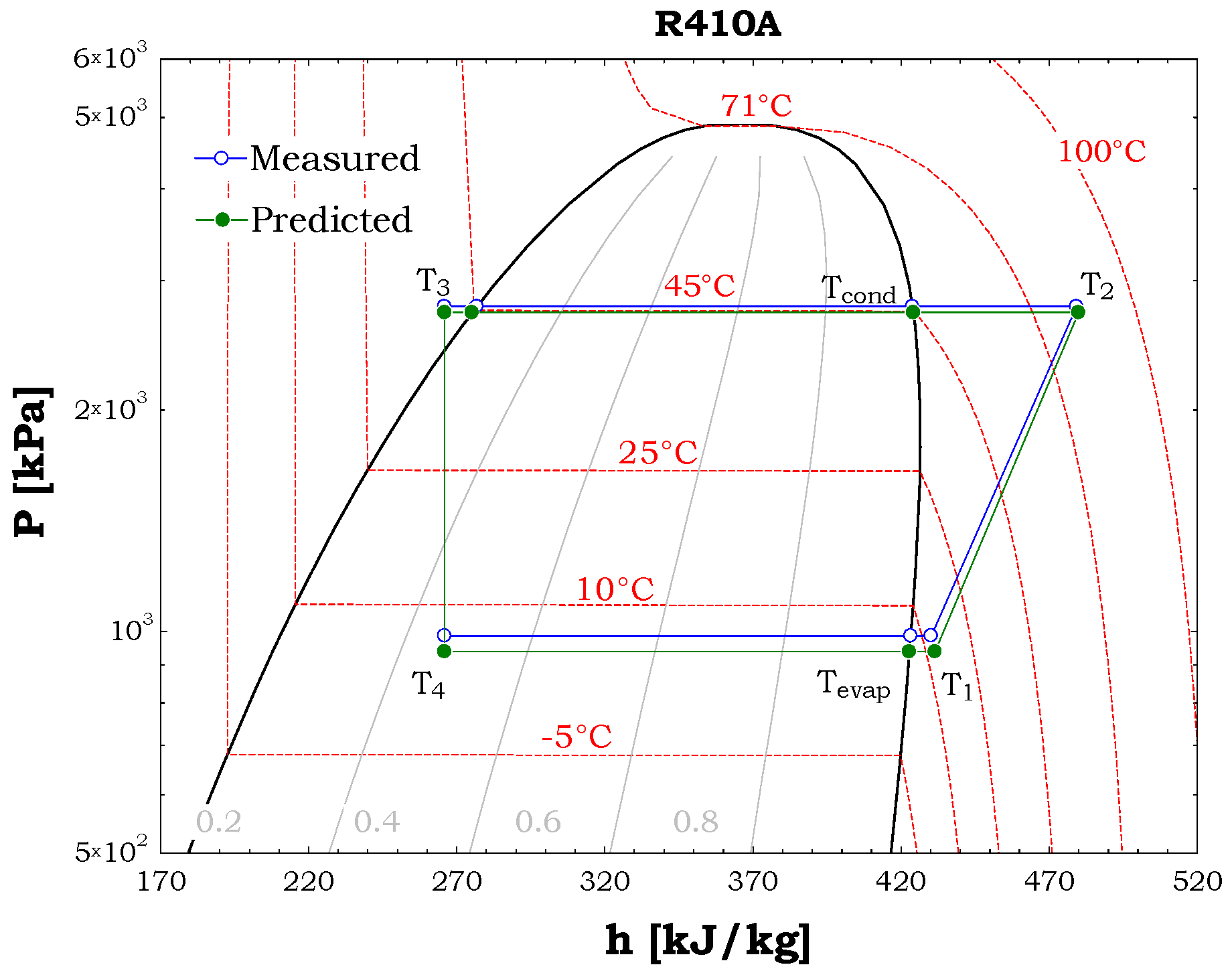
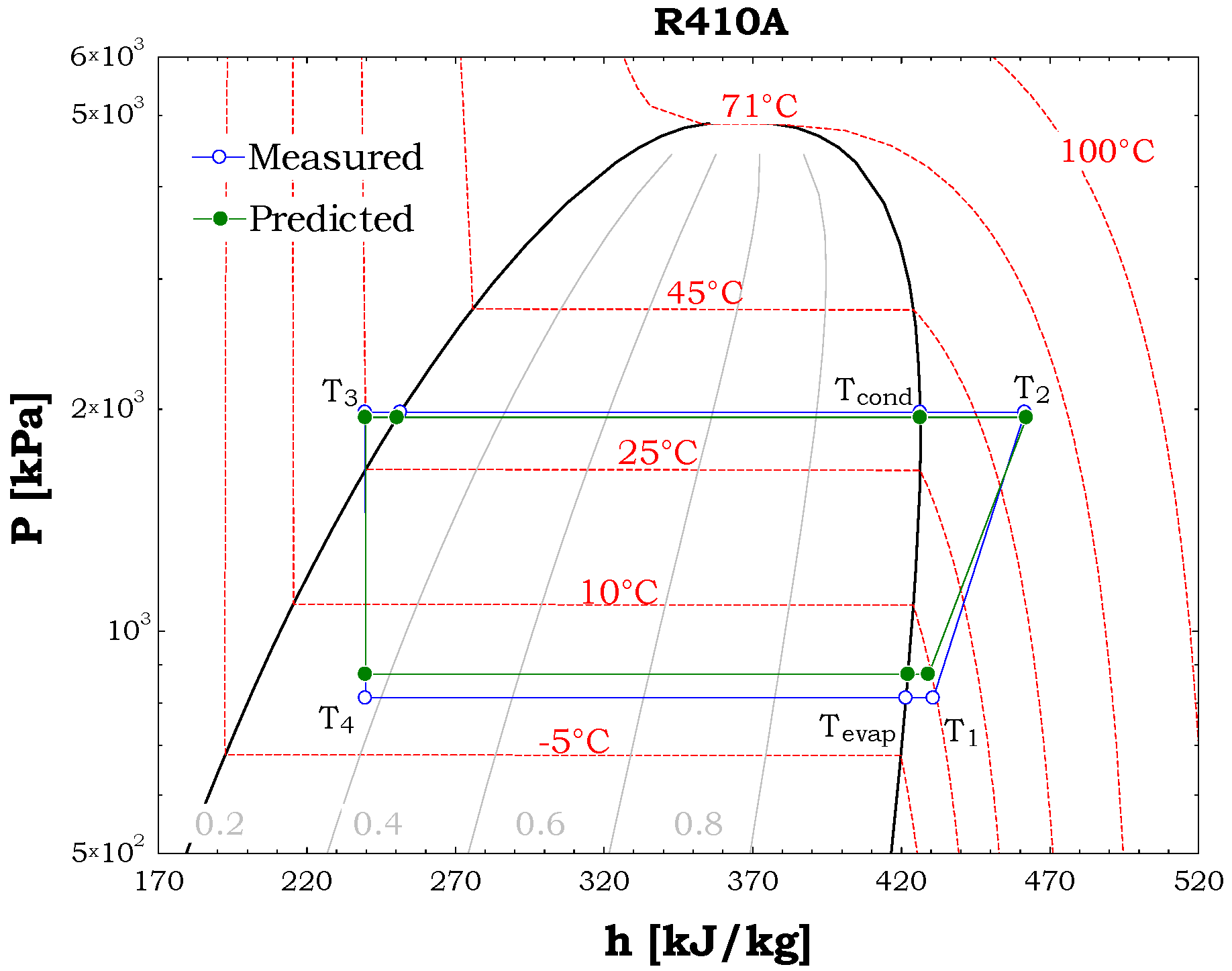
The model can predict several thermodynamic points. For example, Figure 11 and Figure 12 show seven points predicted by the model, and their experimental counterparts, in a P–h diagram for a heating and a cooling case ($T_{{w_S}_{in}}=10 °\mathrm{C}$ and $T_{{w_L}_{in}}=40 °\mathrm{C}$ in the heating case and $T_{{w_S}_{in}}=35 °\mathrm{C}$ and $T_{{w_L}_{in}}=10 °\mathrm{C}$ in the cooling case). As can be seen, the agreement between the model and the experiments is good, with a slight difference observed in the evaporating pressure.

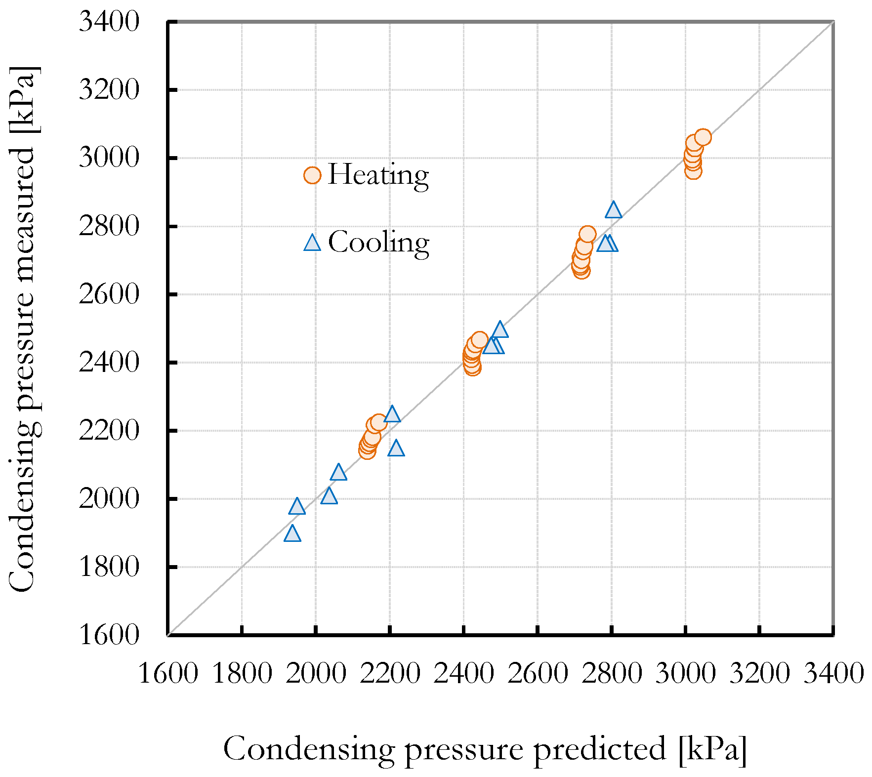
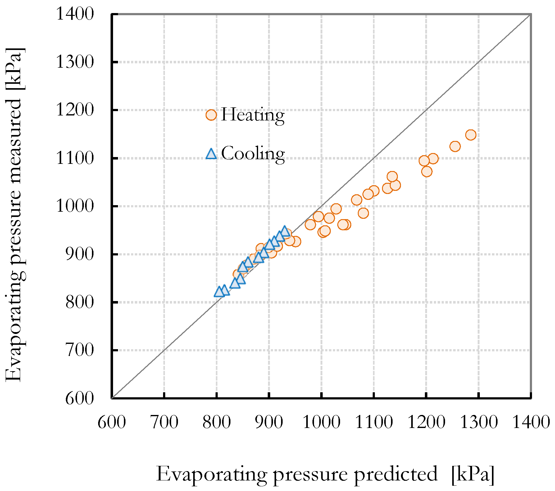
Figure 13 and Figure 14 compare the experimentally measured condensing and evaporating pressures and those calculated using the model. In the case of the condensing pressure, the agreement is good, with an RMSE of 27 kPa and corresponding uncertainties of $\pm 10$ and $\pm$15 kPa for condensing pressures of 2000 and 3000 kPa, respectively. There are noticeable differences between the predictions and the measurements of the evaporating pressure (Figure 14). This discrepancy becomes more pronounced with increasing evaporator temperatures: the absolute error is 10 kPa at low pressures (where the experimental uncertainty is $\pm$4 kPa at 800 kPa) and reaches 100 kPa at higher pressures (the experimental uncertainty is $\pm$6.5 kPa at 1300 kPa). These differences are probably caused by the inability of the expansion valve model to accurately predict the superheat temperature over the full range of conditions. Any error introduced in the computation of the superheat temperature directly influences the forecasted evaporation pressure.

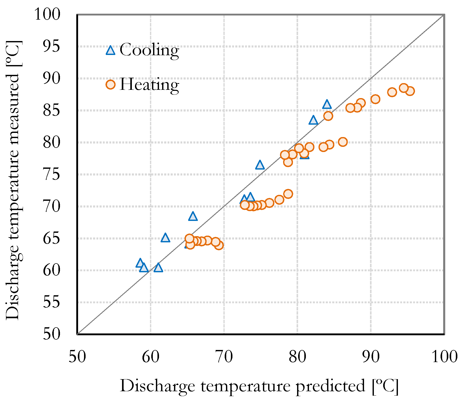
A comparison between the measured and predicted compressor discharge temperatures is presented in Figure 15. The agreement between the model and the experiments is very good in terms of cooling but shows some discrepancies during heating. The data points located significantly away from the diagonal line represent cases with higher $T_{{w_S}_{in}}$ values, indicating a high degree of superheating. A rise in $T_{{w_S}_{in}}$ is associated with an increased error in predicting the evaporation pressure, as indicated in Figure 14. This discrepancy adversely impacts the refrigerant mass flow rate forecast, consequently influencing the compressor’s discharge temperature.

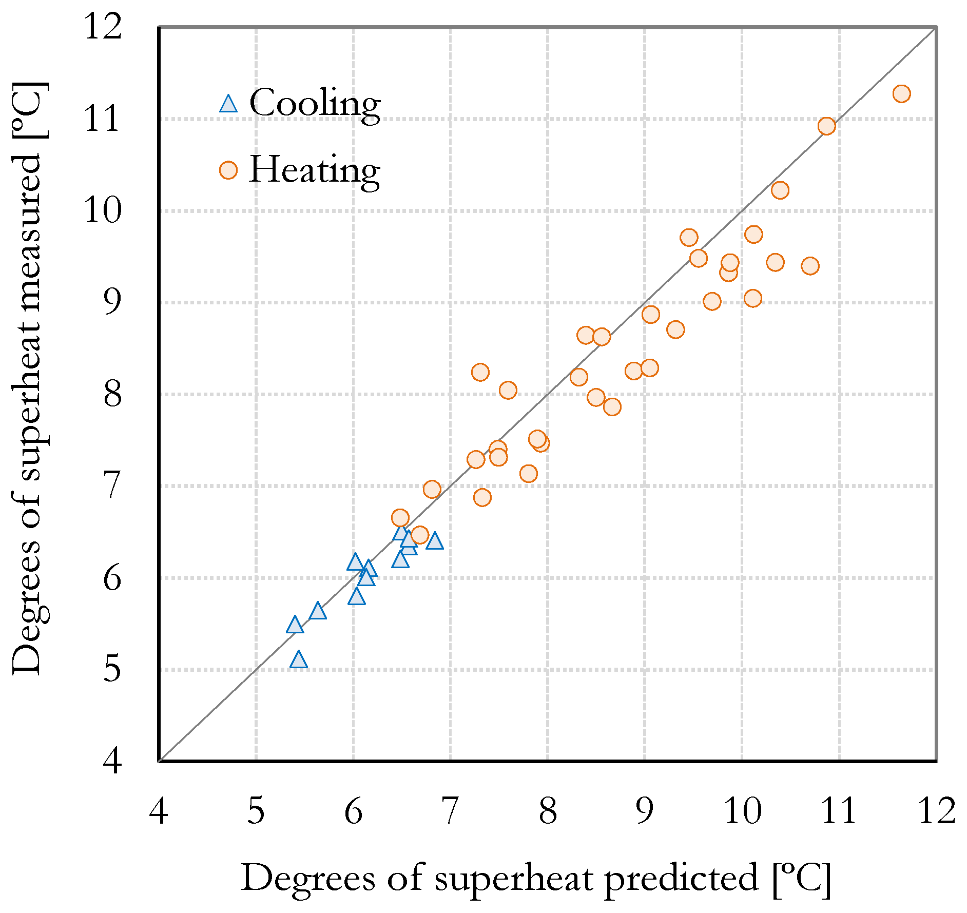
Figure 16 compares the experimentally measured degrees of superheat and those calculated using the model. In heating mode, the data present an RMSE of $\pm$0.54 °C, while it is $\pm$0.14 °C in the cooling mode.

5.3. Non-Operational Conditions

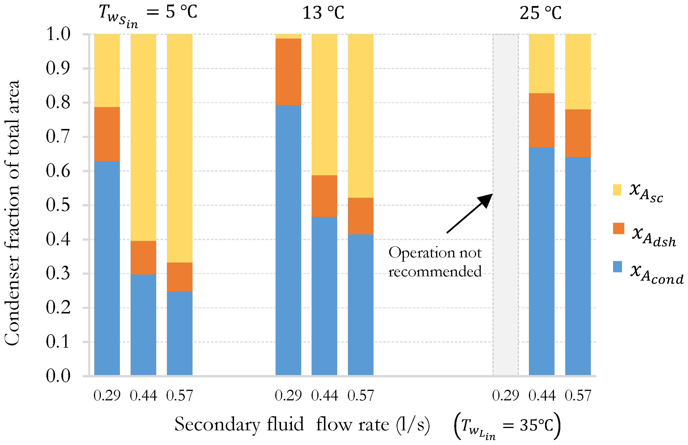
One interesting feature of the present modeling approach is that it is possible to predict non-operational conditions, i.e., operating conditions that are not recommended. Two scenarios that lead to non-operational conditions are examined here. The first one is present in the heating mode, where the refrigerant leaving the condenser has not fully condensed and refrigerant vapor reaches the expansion valve’s inlet, an unwanted condition. The second condition occurs in the cooling mode and is related to high sub-cooling, forcing the expansion valve to operate in the subcooled liquid zone without reaching the vapor–liquid zone.

The first scenario is examined, in Figure 17, for three mass flow rates of the secondary fluids. In each case, the same mass flow rate is employed at both the source and the load: 0.29, 0.44, and 0.57 L/s. The load temperature is held constant at 35 °C, while source temperatures equal to 5, 13, and 25 °C are used.

The figure shows the fraction of the total heat exchanger (condenser) surface area utilized in each zone for desuperheating, $x_{A_{dsh}}$; condensation, $x_{A_{cond}}$; and subcooling $x_{A_{sc}}$. When examining Figure 17 with a focus on $T_{{w_S}_{in}}$, it becomes clear that the proportion of the area allocated to condensation ($x_{A_{cond}})$ grows significantly as $T_{{w_S}_{in}}$ rises. This phenomenon can be attributed to the increase in refrigerant density caused by a higher $T_{{w_S}_{in}}$. Consequently, the mass flow rate from the compressor increases proportionally, resulting in an increased heat pump capacity. The value of $x_{A_{cond}}$ also increases drastically when the mass flow rate of the secondary fluids decreases. As illustrated in Figure 17, when considering a constant temperature, such as $T_{{w_S}_{in}}$ = 13 °C, $x_{A_{cond}}$ changes from 0.4 at a flow rate of 0.57 L/s to 0.8 at a flow rate of 0.29 L/s. An analysis conducted at the pinch point (The point in a heat exchanger where the temperature discrepancy between the cold and hot fluids is at a minimum) results in a difference of 3 °C at high flow rates (0.57 L/s) but only 0.5 °C at low flow rates (0.27 L/s). This directly reduces the value of the ${∆T}_{l{m}_{cond}}$ in the zone, and, consequently, a larger heat transfer area is required for condensation.

Similarly, the portion of the surface area dedicated to desuperheating expands in proportion to the rising $T_{{w_S}_{in}}$ temperature. This gradual expansion, however, leads to a diminishing amount of available surface area for sub-cooling.

It is clear that elevating the $T_{{w_S}_{in}}$ and decreasing the $\dot{m}$ can result in an inadequate heat exchange surface area for sub-cooling. This observation is notable in the case of 0.29 L/s and $T_{{w_S}_{in}}$ = 13 °C, where the surface area fraction $x_{A_{sc}}$ is nearly negligible. Beyond this temperature, $x_{A_{sc}}$ reduces to zero, indicating that the refrigerant has not fully condensed, potentially causing issues with the expansion valve’s operation. The prediction of $x_{A_{sc}}$ = 0 is compared to the manufacturer’s operating condition recommendations. This comparison with heating is shown in

Table 5. Heat pump’s non-operational conditions, according to the manufacturer, in its heating mode.

Source		Load (Cooling)		Manufacturer Recommendation	$\mathbf{Prediction} \mathbf{of} {\mathit{x}}_{{\mathit{A}}_{\mathit{s}\mathit{c}}}=0$ by the Model
EWT [°C]	L/s	EWT [°C]	L/s
15.5	0.284	54.4	0.284	Operation not recommended	yes
	0.429
	0.568
21.1	0.284	54.4	0.284	Operation not recommended	yes
	0.429
	0.568
26.7	0.284	54.4	0.284	Operation not recommended	yes
	0.429
	0.568

. As seen in these tables, the model can predict the operating conditions not recommended by the manufacturer.

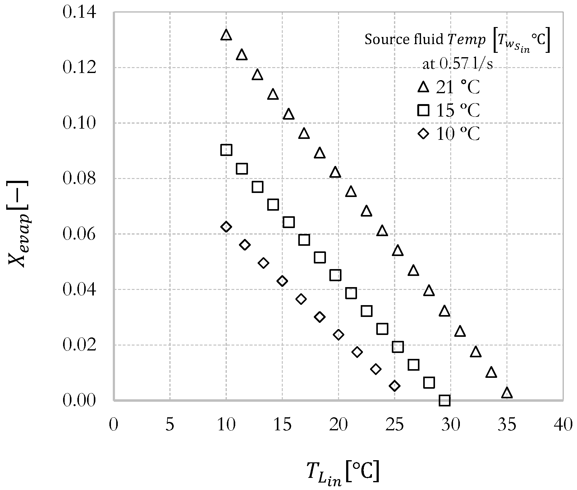
A thermal expansion valve (TEV) is a crucial component in a refrigeration system. The main objectives of the TEV are to regulate the refrigerant’s flow into the evaporator and maintain proper superheat. The thermal expansion valve typically operates in the liquid–vapor zone rather than the liquid–liquid zone. Operating a TEV in the liquid–liquid zone is generally not desirable. It might result in insufficient evaporation, leading to issues like liquid slugging (liquid entering the compressor), reduced system efficiency, and potential damage to the compressor. This situation is evaluated in the second scenario. Under typical conditions, the refrigerant enters as subcooled liquid and exits the expansion process with a certain vapor quality. Figure 18 shows the quality with which the refrigerant leaves the expansion valve before entering the evaporator for three constant temperatures of $T_{{w_S}_{in}}$: 10, 15, and 22 $°\mathrm{C}$. It can be observed that as the return temperature of the load, $T_{{w_L}_{in}},$ increases, the refrigerant quality tends towards zero, indicating that the TEV will operate in the liquid–liquid zone.

The prediction of a value equal to zero ($X_{evap}=0)$ is compared to the manufacturer’s operating condition recommendations. This comparison for cooling is shown in

Table 6. Heat pump’s non-operational conditions, according to the manufacturer, in its cooling mode.

Source		Load (Cooling)		Manufacturer Recommendation	$\mathbf{Prediction} \mathbf{of} {\mathit{X}}_{\mathit{e}\mathit{v}\mathit{a}\mathit{p}}=0$ by the Model
EWT [°C]	L/s	EWT [°C]	L/s
10	0.44	32	0.44	Operation not recommended	yes
			0.57
	0.57	32	0.44
			0.57
15	0.29	32	0.44	Operation not recommended	yes
			0.57
	0.44	32	0.44
			0.57
	0.57	32	0.44
			0.57
22	0.29	32	0.44	Operation not recommended	yes
			0.57
	0.44	32	0.44
			0.57
	0.57	32	0.44
			0.57

. As seen in these tables, the model can predict the operating conditions not recommended by the manufacturer.

6. Conclusions

This research introduces and provides experimental validation for a steady-state model of water-to-water heat pumps. The primary objective of the model is to estimate the heat pump’s capacity (heating or cooling) and necessary compressor power, given the specified inlet conditions of the secondary fluids on both the load and source sides. The heat pump model includes a detailed representation of the evaporator and condenser, which are both formed of plate heat exchangers. The fixed-speed scroll compressor is modeled using manufacturer performance maps, and a new semi-empirical model is introduced for the thermostatic expansion valve, accounting for the effects of condensing temperature on superheating prediction.

The assembly of sub-models for individual components results in a global model, leading to a set of nonlinear equations solved using an equation solver and appropriate guess values. The complexity of solving this model arises from the nonlinearity of the equations representing its thermodynamic and physical phenomena, coupled with the permissible operational conditions linked to the design of each component.

The validation of this model is carried out in an experimental test facility, utilizing precisely controlled secondary fluid loops for the secondary fluids’ temperature and flow rate. The results demonstrate good agreement between the complete heat pump model predictions and experimental data in both the heating and cooling modes. The comparison includes power consumption, coefficients of performance (COPs), and various operational conditions such as evaporating and condensing temperatures, degrees of superheat, and compressor discharge temperatures.

In the assessed scenarios, the coefficient of performance (COP) ranges from 3.7 to 7.5 in the heating mode and 3.2 to 5.7 in the cooling mode. The COP can double when the temperature difference between the secondary fluids decreases from 35 °C to 10 °C. The model’s COP predictions fall within the limits of experimental uncertainty in every case. It is also shown that an increase in the difference between the source and sink inlet temperatures leads to an increase in the required compressor power, and thus lower COPs. However, variations in the source inlet temperature have a relatively minor impact on the required compressor power.

Noted discrepancies between the model and experiments are likely due to the expansion valve model’s limitations in precisely predicting the superheat temperature across all conditions. Any inaccuracies in calculating the superheat temperature directly affect the predicted evaporation pressure. This divergence is more noticeable at higher evaporator temperatures: at lower pressures, the absolute error is 10 kPa (with an experimental uncertainty of ±4 kPa at 800 kPa), and it escalates to 100 kPa at higher pressures (where the experimental uncertainty is ±6.5 kPa at 1300 kPa).

The model can predict cases where the surface area for subcooling vanishes to zero, indicating that the refrigerant has not fully condensed, potentially causing issues with the expansion valve’s operation. The predictions of these non-operational conditions match the manufacturer’s recommendations.

The model validation was conducted based on specific parameters, including the heat pump’s size and operational conditions. Further investigations are recommended for various sizes of heat pumps, along with experimental conditions that allow for the confirmation of non-operational scenarios and improvements to the proposed sub-model for the TEV.

The model has promising applications in various practical contexts. These include assessing the efficiency of new refrigerants, the sizing of plate heat exchangers, gathering performance data to develop performance maps for use in building energy simulation software, and predicting undesirable non-operational states, among others.