Methodology for Multi-Step Forecasting of Electricity Spot Prices Based on Neural Networks Applied to the Brazilian Energy Market

Abstract

Forecasting electricity spot prices holds paramount significance for informed decision-making among energy market stakeholders. This study introduces a methodology utilizing a multilayer perceptron (MLP) neural network for multivariate electricity spot price prediction. The model underwent a feature selection process to identify the most influential predictors. In the validation phase, the model’s performance was evaluated using key metrics, including trend accuracy percentage index (TAPI), normalized root mean squared error (NRMSE), and mean absolute percentage error (MAPE). The results were obtained for a four-week forecast horizon in order to serve as an auxiliary tool to facilitate decision-making processes in the short-term energy market. The relevance of short-term electricity spot price forecasting lies in its direct impact on pricing strategies during energy contract negotiations, which allows for the making of assertive decisions in the energy trading landscape.

1. Introduction

In recent decades, numerous countries have witnessed substantial transformations in their electrical power sectors driven by the necessity to introduce market mechanisms and stimulate competition among industry stakeholders [1]. In the case of Brazil, this restructuring introduced new entities like the National Agency of Electrical Energy (ANEEL), the National System Operator (ONS), and the Chamber of Commercialization of Electric Energy (CCEE).

The shift from a monopolistic pricing model to a competitive environment saw the emergence of two trading environments: the Regulated Contracting Environment (ACR) and the Free Contracting Environment (ACL) [2]. In the ACR, electrical energy procurement occurs through ANEEL-promoted auctions that involve generator and distributor agents. Conversely, in the ACL, contracts are negotiated among generator agents, marketers, and free consumers. This setup allows for flexibility in negotiating both energy volume and prices.

All energy contracts in Brazil, whether in the ACL or the ACR, must be registered with the CCEE. Additionally, energy generation and consumption measurements are recorded. These registrations account for differences between contracted and actual energy volumes, which are traded in the short-term market under the Price for Differences Settlement (PLD), also known as the electricity spot price [2,3].

An assertive spot price projection provides a vision of the future regarding possible energy conditions, prices, and the impact of these factors together on the commercialization sector [2]. It is important to highlight that the trend in the PLD directly influences ACL and ACR contract prices, making spot price projection an important strategy for energy trading in the Brazilian electrical sector.

Traditionally, the calculation of the PLD derives from the operation planning of the electrical system and represents the minimum cost in BRL/MWm to increase a unit of load in the system. In Brazil, ONS and CCEE calculate this value using the DECOMP [4] model, which also provides the short-term projection of the electricity spot price. DECOMP calculates the spot price through a combined representation of hydroelectric and thermoelectric plants and aims to estimate the minimum operation cost. This methodology is based on a stochastic dual dynamic programming (SDDP) approach, which aims to improve decisions made in environments with uncertainty over time [5].

However, the DECOMP model is computationally intensive, requiring a large amount of data and time for processing. In addition to the huge computational effort, the price projection provided by DECOMP does not always correspond to the reality. Given this scenario, other alternatives have been studied to overcome and improve the accuracy of the spot price projection. References [6,7,8] offer an overview of a variety of forecasting techniques with a focus on forecasting electricity prices.

In the literature, there are works based on statistical analysis and implementation for energy price projection [9,10,11]. However, in the Brazilian scenario, the application of statistical methods to estimate energy prices faces significant challenges, primarily due to their complexity in dealing with nonlinear relationships. The presumption of a direct linear correlation between input and output variables contrasts with the intricate dynamics of the energy market, which are characterized by nonlinear relationships. Other studies, in turn, suggest the implementation of models based on machine learning to capture patterns in historical data and, thus, estimate the electricity price [12,13,14,15,16,17,18,19,20,21]. Several of them highlight the use of artificial neural networks [15,16,17,18,19,21], which are capable of dealing with noisy or imprecise data and capturing nonlinear relationships between input variables.

After a literature review, it was found that the majority of works related to energy price forecasting focus on hourly energy predictions for the next day [9,12,13,14,15,16,17,18,20]. However, this research proposes a price forecasting model based on weekly intervals. The hourly price forecast approach can be valuable for energy market operators who need to make decisions in the very short term to allow for more precise resource allocation and reducing load usage during periods of higher prices. On the other hand, the weekly forecast of energy prices provides a more comprehensive view of price behavior by encompassing trends and patterns in the short and medium terms. Moreover, a weekly forecast can help manage the risk of fixed-price energy contracts by anticipating changes in market conditions, which facilitates strategic decision-making, such as the choice of contracts and investment decisions.

Furthermore, in this study, we aim to present the model’s outcomes across test periods linked to diverse energy conditions. One of the main limitations identified in several studies concerning energy price forecasting is related to the size of the test data, which are often small in size [11,14,15,16,17]. This issue may compromise the evaluation of the algorithms’ performance, especially in special conditions that may impact the energy market. The volatility observed in electricity spot price windows underscores the need for adaptable modeling methods.

In this context, this study contributes by presenting a methodology based on machine learning to estimate short-term spot energy prices at weekly intervals, providing an alternative to the traditional forecasts offered by the DECOMP model in Brazil. For this purpose, a model relying on an artificial neural network with a multilayer perceptron architecture is employed. The methodology utilizes cross-validation to assess the model under diverse energy conditions, including periods of extreme prices, providing an understanding of its performance in the face of unforeseen changes in the energy environment. Validation periods encompass the years 2021 and 2022, and model evaluation is conducted using performance metrics such as MAPE, NRMSE, and TAPI calculated over the price time series.

2. Artificial Neural Networks

Artificial neural networks are computational techniques that present a mathematical model inspired by the neural structure of the human brain and that acquire knowledge through experience. These networks feature basic processing units that are called neurons.

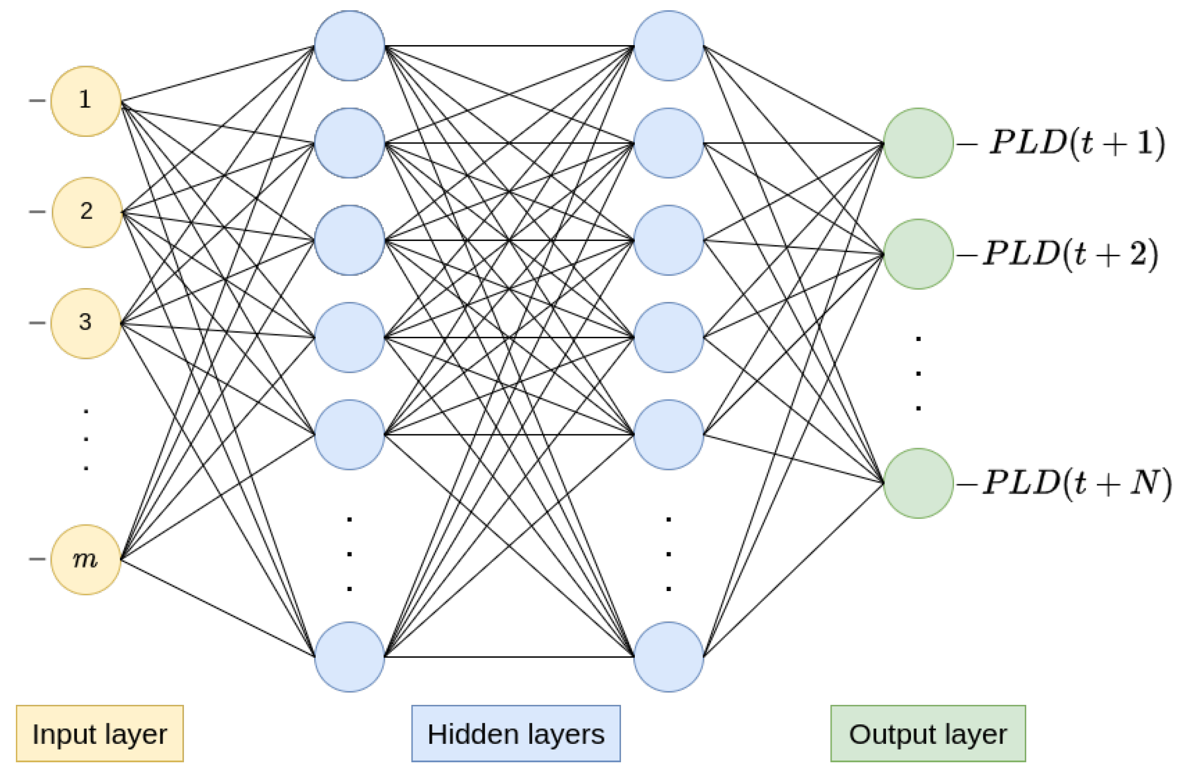
One of the most commonly used neural network architectures in time series prediction is the multilayer perceptron (MLP) thanks to its ability to handle the nonlinear and dynamic characteristics that frequently arise in this type of problem [21]. MLP consists of a neural network architecture that features a layer of input neurons, one or more hidden layers, and a layer of output neurons. The output layer receives stimuli from the intermediate layer and generates the response to the problem. Meanwhile, the intermediate layers are capable of extracting features from the data and identifying patterns within it. In the short-term market, MLP can be used to predict the spot price over a given prediction horizon in the case of a multi-step forecast, like in Figure 1.

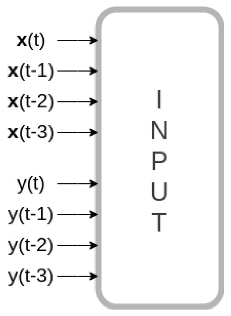
The input layer incorporates m neurons to process the input data. In order to predict the electricity spot price, several combinations of regressor variables were tested, including hydraulic, thermal, wind, and solar generation; natural affluent energy; energy stored in reservoirs; as well as fossil fuel prices. Additionally, historical values of these variables over time and past values of electricity spot prices themselves were incorporated as input variables, as depicted in Figure 2. The configuration of hidden layers and neurons per layer varies based on the problem’s complexity [22]. Neural networks with two hidden layers can represent functions with any kind of shape, but for most problems involving the use of neural networks with MLP architecture, one hidden layer may be enough [22]. Finally, the output layer is used to predict energy prices for desired N time steps.

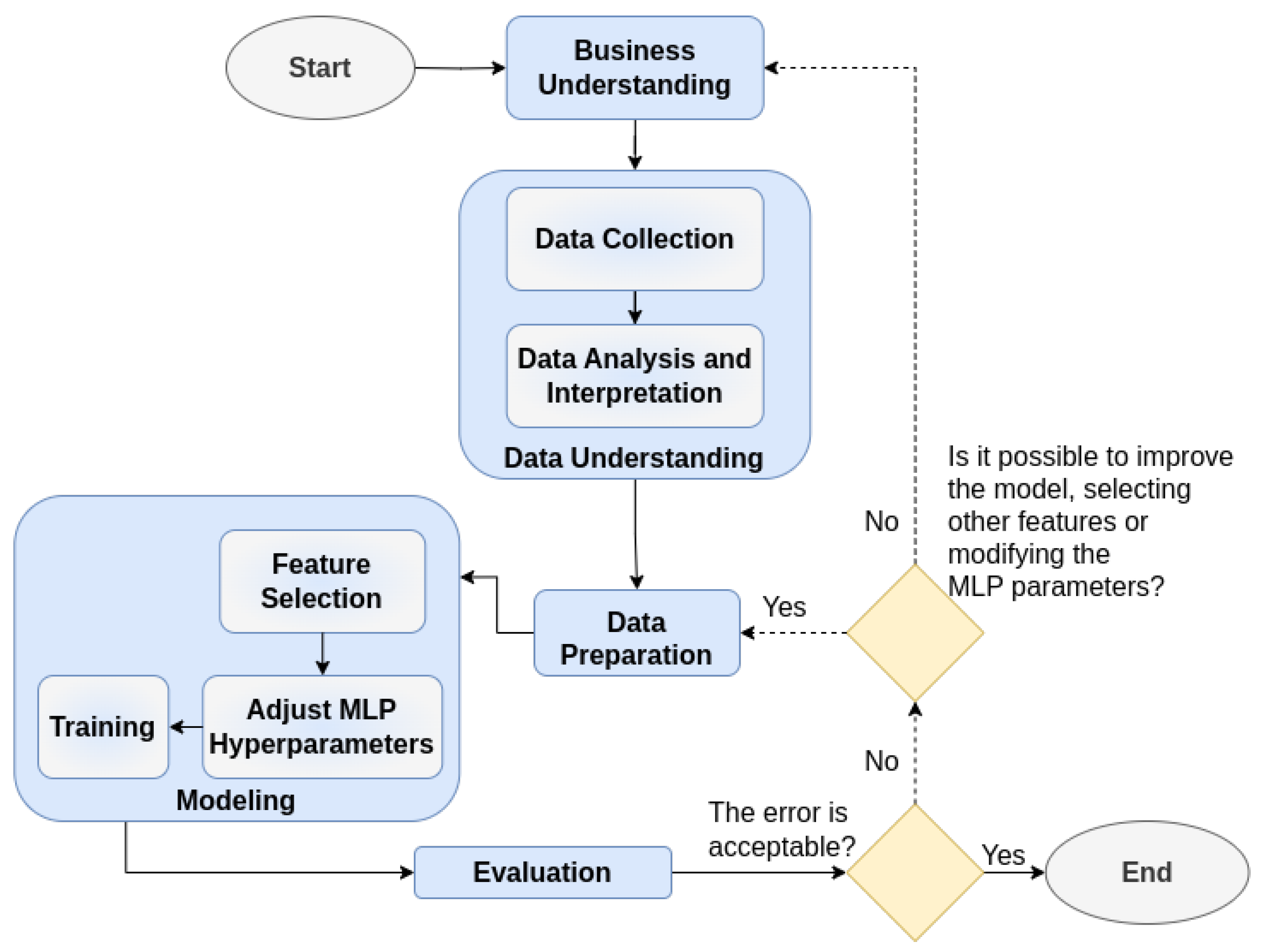
The development of this work is based on the CRISP DM methodology (Cross Industry Standard Process for Data Mining). This methodology provides a uniform structure and guidelines for data science flow. It consists of six phases, namely: business understanding, data understanding, data preparation, modeling, evaluation, and deployment [23]. The proposed methodology will be applied to estimate the electricity spot price in Brazil, offering valuable insights to market stakeholders for making informed decisions. To achieve this goal, the methodology employed in this study is illustrated in Figure 3.

2.1. Business Understanding

During this phase, efforts were made to comprehend the dynamics of the energy market (in our case, the Brazilian market) and its particularities, including the main factors that influence the electricity spot prices, in addition to the specific demands of market stakeholders. Through this analysis, it is possible to define the scope of the research, identify which variables and data are most relevant for modeling, and choose the most appropriate analytical approaches to face market challenges.

2.2. Data Understanding

The data understanding phase involves collecting, exploring, and gaining initial insight into the available data and identifying patterns and quality issues. In the context of estimating energy spot prices, this phase involves a more in-depth examination of datasets that are specifically pertinent to energy prices, with the aim of uncovering factors that could enhance forecast accuracy. The goal is to obtain a clear understanding of the data to guide the subsequent steps of the methodology.

In the data understanding phase of the CRISP-DM methodology, the exploration and analysis of data take center stage. Within the scope of estimating energy prices in the Brazilian context, this phase involves delving into datasets that are specifically relevant to energy price estimation. The goal is to gain insights into the nature, quality, and potential patterns within these datasets, recognizing their direct relevance to the subsequent steps of the energy price estimation process.

2.2.1. Data Collection

The electricity spot price in Brazil is defined for each submarket (North, South, Northeast, and Southeast/Central-West) and also by load level (light, medium, and heavy), representing different levels of electricity consumption. For this work, the aim was to estimate spot prices for the Southeast/Central-West subsystem with the average consumption level. This subsystem was selected because it represents the largest contribution of installed power in Brazil. To collect the necessary data, historical price records available on the CCEE and ONS websites were accessed. The ONS also provides for each submarket data relating to:

• ENA (natural affluent energy): energy available from natural water flow into hydroelectric plant reservoirs;
• EAR (energy stored in reservoirs): potential energy stored in reservoirs for electricity conversion;
• Consumption data;
• Generation data (hydraulic, thermal, wind, and solar);
• CVU (unit variable cost): average variable production cost per unit of electrical energy from thermal plants.

2.2.2. Data Analysis and Interpretation

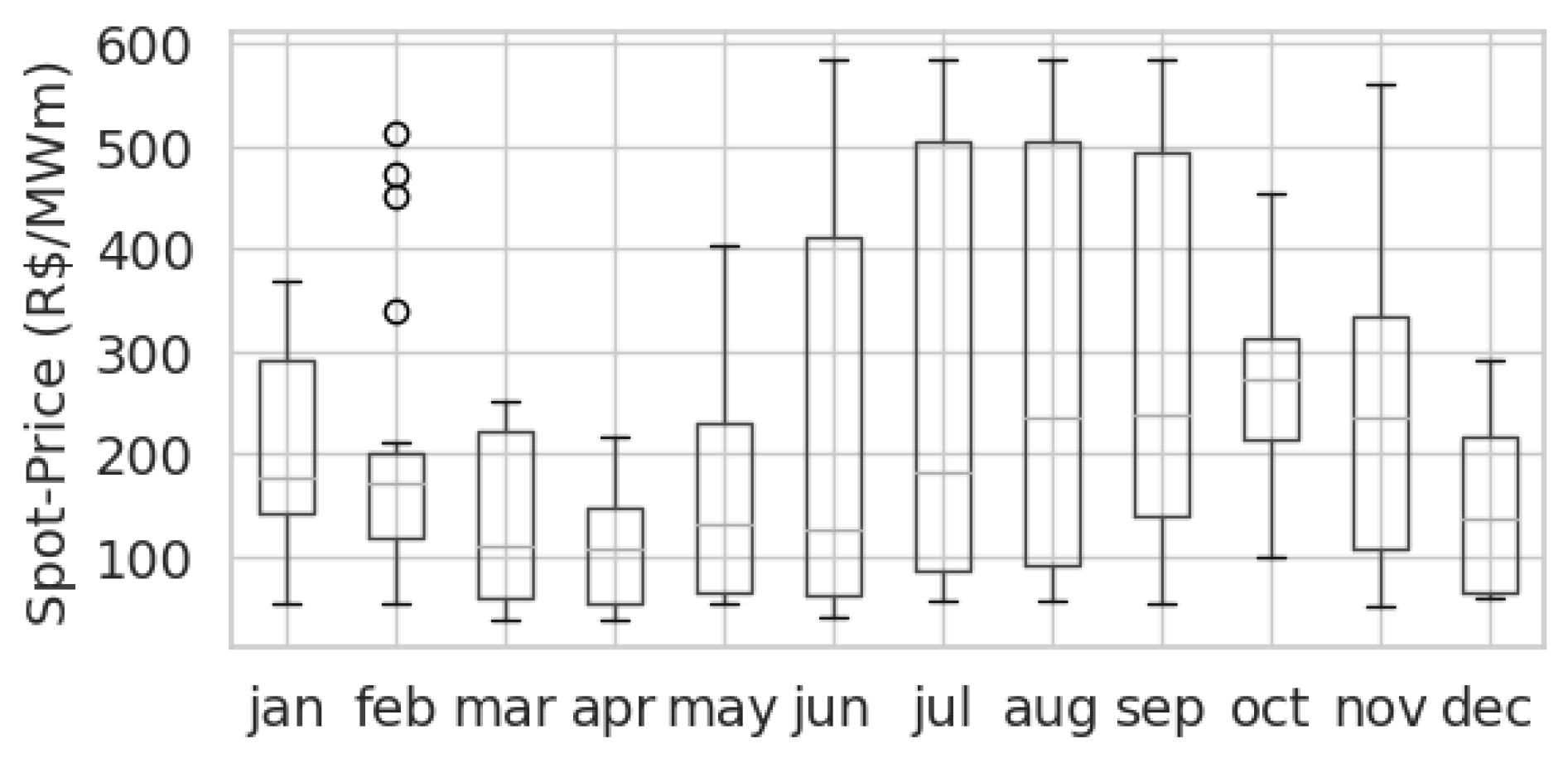
The variation in energy prices for each month throughout the captured time window is depicted in Figure 4.

Significant weekly price volatility is observed, evidenced by the notable difference between quartile values. This indicates a high dispersion of spot prices throughout the weeks. Furthermore, the median in Figure 4 indicates a price growth trend at the beginning of the second semester, followed by a decline towards the end of the year within the employed time window.

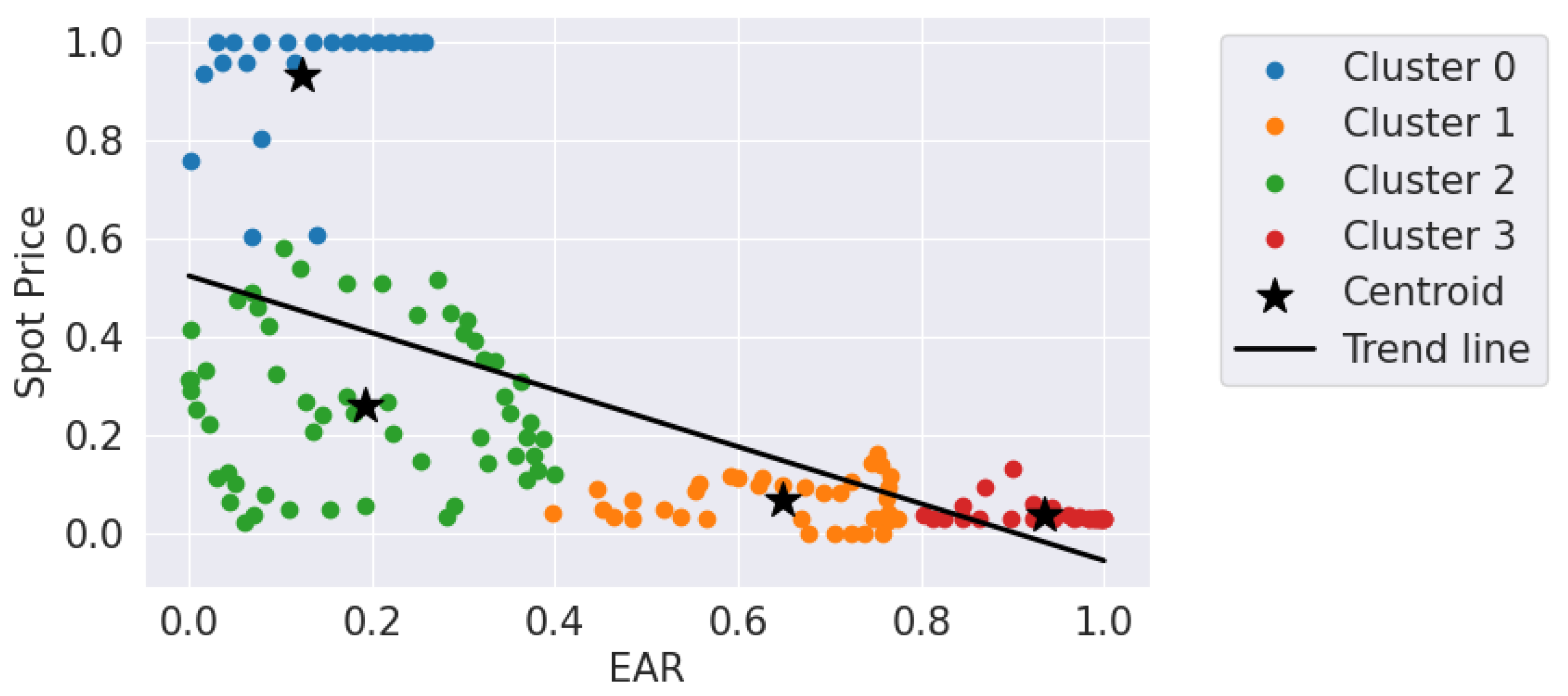
In addition to the spot price, other features were analyzed to be used as regressors for the model. Figure 5 displays a scatter plot that illustrates the relationship between EAR in the Southeast/Central-West region and the energy price in this submarket. To analyze this relationship, a data clustering process was conducted to group observations sharing similar characteristics.

When examining cluster 3, it is observed that the abscissa of this centroid is situated at higher values of EAR, while the ordinate is positioned at lower values of spot price. Conversely, when analyzing cluster 0, it is noted that the abscissa of this centroid is located at lower values of EAR, while the ordinate is associated with higher values of spot price. These observations suggest a negative relationship between EAR and spot price. The trend line present in the graph emphasizes the inverse association.

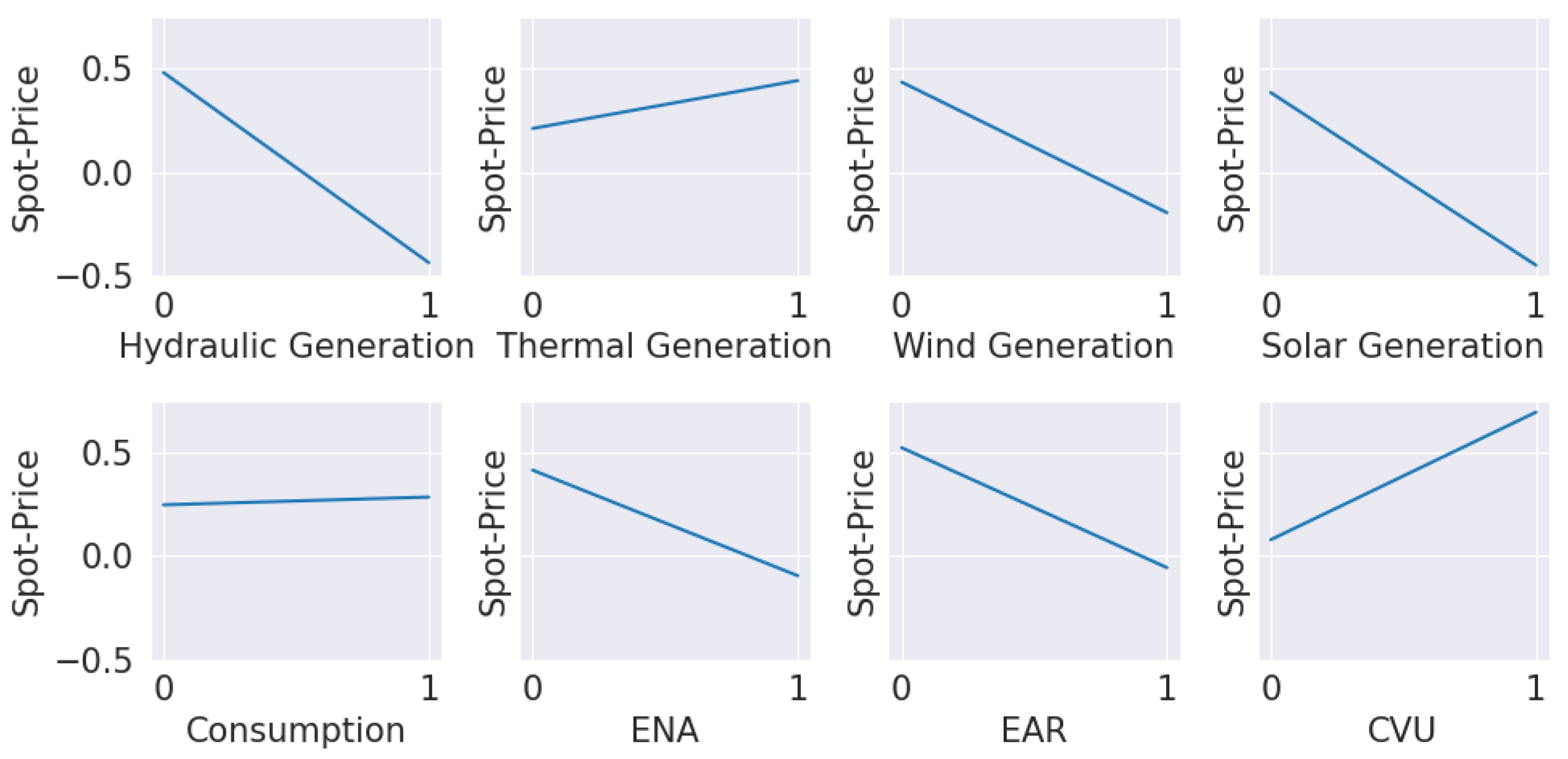
Figure 6 shows the trends of the other features in relation to electricity prices in the Southeast/Central-West region. A positive relation is evident between the energy price and the CVU or thermal generation variables. The other features exhibit a negative relation.

2.3. Data Preparation

Before the modeling process, the data were normalized according to (1). In this way, the MLP can be trained without its parameters being biased towards attributes with larger scales.

$$Z_i=\frac{X_i-\mathtt{min}\left(X_i\right)}{\mathtt{max}\left(X_i\right)-\mathtt{min}\left(X_i\right)}i\in [1,m].$$

(1)

2.4. Modeling

2.4.1. Feature Selection

Analyzing the correlation between attributes helps prevent multicollinearity among variables, in which independent variables are strongly correlated. Multicollinearity can lead to instabilities in the model results and difficulties with interpreting the effects of the variables. Essentially, strongly correlated variables can, to some extent, convey the same information, making it unnecessary to use them jointly.

To identify multicollinearity, the Pearson correlation coefficient can be used. If the absolute value of the linear correlation coefficient is close to 0.8, collinearity is likely to exist [25]. During model development, one variable was selected for each pair of variables that had a Pearson correlation coefficient exceeding 80%.

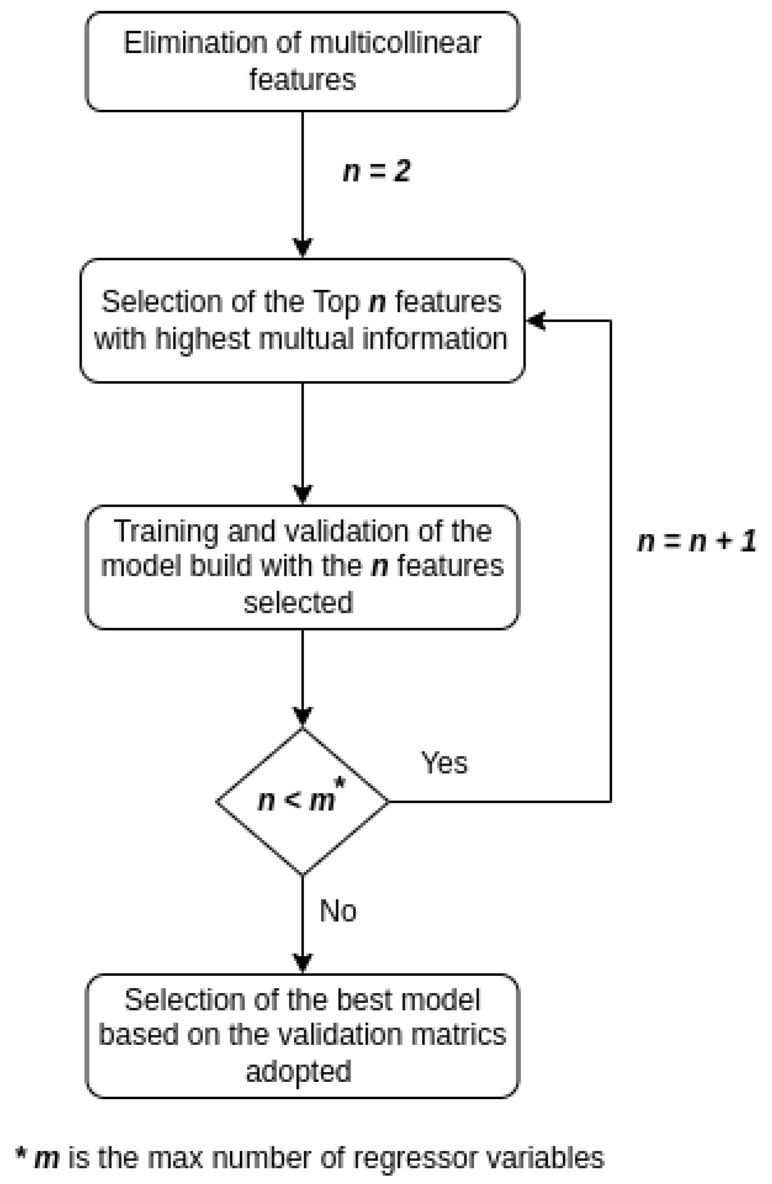
Another useful tool in the feature selection process is the calculation of mutual information, which measures statistical dependence between variables, including nonlinear correlations between attributes and the output variable. This information is used to rank attributes in terms of their relevance for forecasting [26]. After organizing the input features in descending order based on mutual information, the most relevant features for the model were selected.

Table 1. Features’ mutual information values.

Rank	Mutual Info.	Regressor Variable
1	0.6966	EAR (SE)
2	0.6685	Thermal Generation—Fuel Oil (SIN)
3	0.6615	Thermal Generation (SE)
4	0.5957	Thermal Generation—Gas (SIN)
5	0.5518	Solar Generation (SE)
6	0.5515	Thermal Generation—Gas (S)
7	0.5479	Thermal Generation (NE)
8	0.5478	Thermal Generation (N)
9	0.5378	Thermal Generation (S)
10	0.5285	Thermal Generation—Industrial Waste (S)

provides an example with the 10 regressor variables with the highest mutual information values.

Subsequently, a range of prediction models was trained and tested, each incorporating a varying number of chosen attributes, as illustrated in Figure 7.

2.4.2. Adjusting MLP Hyperparameters

The definition of the MLP architecture involved choosing the number of intermediate layers as well as the number of neurons in these layers. The number of neurons in the input and output layers were defined depending on the number of features selected n the preceding step and the number of desired predictions, respectively. As the objective is to predict the spot price in the Southeast/Central-West up to four weeks ahead, four neurons were adopted in the output layer.

Two hidden layers were instantiated so that the network could learn the high nonlinearities present in the relationships between the input variables and the spot price. The number of neurons in the hidden layers was set to $2·m$, where m is the number of selected attributes [22]. Therefore, each candidate model presented a unique MLP structure since the number of attributes per model was different. Consequently, the number of neurons per intermediate layer also varied.

2.4.3. Training

The candidate models were trained using the limited-memoryBFGS (LBFGS) optimization algorithm. For the proposed problem, LBFGS presents itself as a good alternative as it can deal well with optimization problems for which the amount of training data is relatively small (hundreds of samples). Therefore, this method tends to converge faster and have better performance when compared to other algorithms [27].

2.5. Evaluation

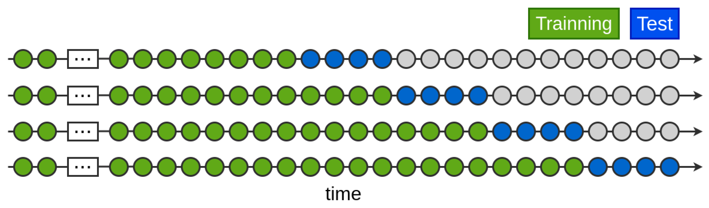
During the validation stage of the candidate models, time series cross-validation was employed. This approach involves using a set of test samples, each consisting of four observations (model-estimated steps), with the training set encompassing all samples prior to the test set. Figure 8 depicts this validation method.

Cross-validation allows assessment of the effectiveness of the model’s structure since it enables validation under different market conditions, as each test set belongs to a distinct time window of the year. For each test sample, the model’s performance was evaluated using the performance metrics mean absolute percentage error (MAPE) (2), normalized root mean squared error (NRMSE) (3), and trend accuracy percentage index (TAPI) (4). While MAPE and NRMSE are error metrics, TAPI is an indicator created to measure forecast trend accuracy.

$$\mathrm{MAPE}=\frac{1}{N}\sum _{i=1}^N\frac{\left|y_i-{\widehat{y}}_i\right|}{max\left(ϵ,\left|y_i\right|\right)}·100\%,$$

(2)

$$\mathrm{NRMSE}=\frac{\sqrt{\frac{1}{N}{\sum }_{i=1}^N{\left(y_i-{\widehat{y}}_i\right)}^2}}{\overline{y}},$$

(3)

$$\mathrm{TAPI}=\frac{{\sum }_{i=1}^N{\mathrm{TA}}_i}{N}\times 100,$$

(4)

$${\mathrm{TA}}_i=\left\{\begin{array}{cc}1,\hfill & \mathrm{if}\mathrm{sign}({\widehat{y}}_i-{\widehat{y}}_{i+1})=\mathrm{sign}(y_i-y_{i+1}),\hfill \\ 0,\hfill & \mathrm{otherwise}.\hfill \end{array}\right..$$

where $\widehat{y}$ is the predicted value, y is the actual value, $\overline{y}$ is the mean of the actual value, N is the number of test observations, $ϵ$ is a very small value to avoid division by zero, and $T{A}_i$ is a binary variable related to the correctness of the trend for sample i.

3. Results

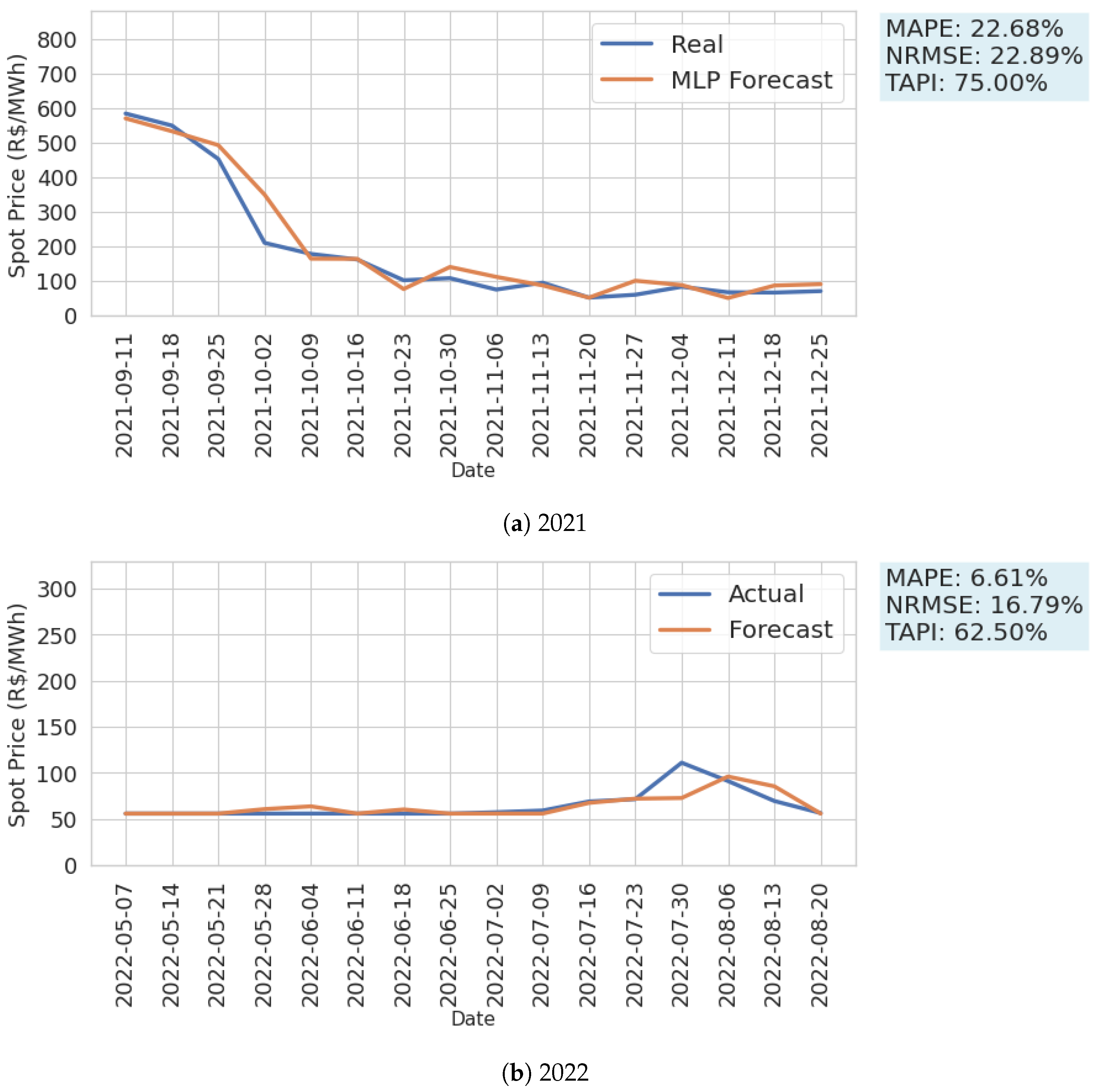
The MLP model that exhibited the best performance was the one for which the exogenous variables EAR (SE/CO), Thermal Generation (SE/CO), Thermal Generation—Gas (SIN), and Thermal Generation—Fuel Oil (SIN) were considered. Additionally, the lagging values of these attributes from the prior three weeks were taken into account as inputs to the model. In Figure 9, the spot price forecast results generated by this model for the years 2021 and 2022 are depicted in windows of 16 weeks each.

Considering the Brazilian energy landscape’s potential for rapid changes, cross-validation serves as a valuable tool. Over recent years, the market has witnessed unconventional scenarios, transitioning from price windows near the maximum values established in 2021 to periods closer to the minimum in 2022. This trend persisted throughout 2023, with prices remaining consistently low due to favorable hydrological conditions. Consequently, the decision was made to test the model in 2021 and 2022 to evaluate its performance under different energy scenarios.

In the cross-validation process, temporal data are divided into consecutive segments, as illustrated in Figure 8. The model is then trained with historical data from the first week of 2016 up to a certain point in time, known as the cutoff. Subsequently, the model is employed to predict out-of-sample values in the test set. These out-of-sample predictions are then compared with the actual values to evaluate the model’s performance when forecasting future unseen values. The process is repeated across the entire temporal series by sliding the training and test windows over time.

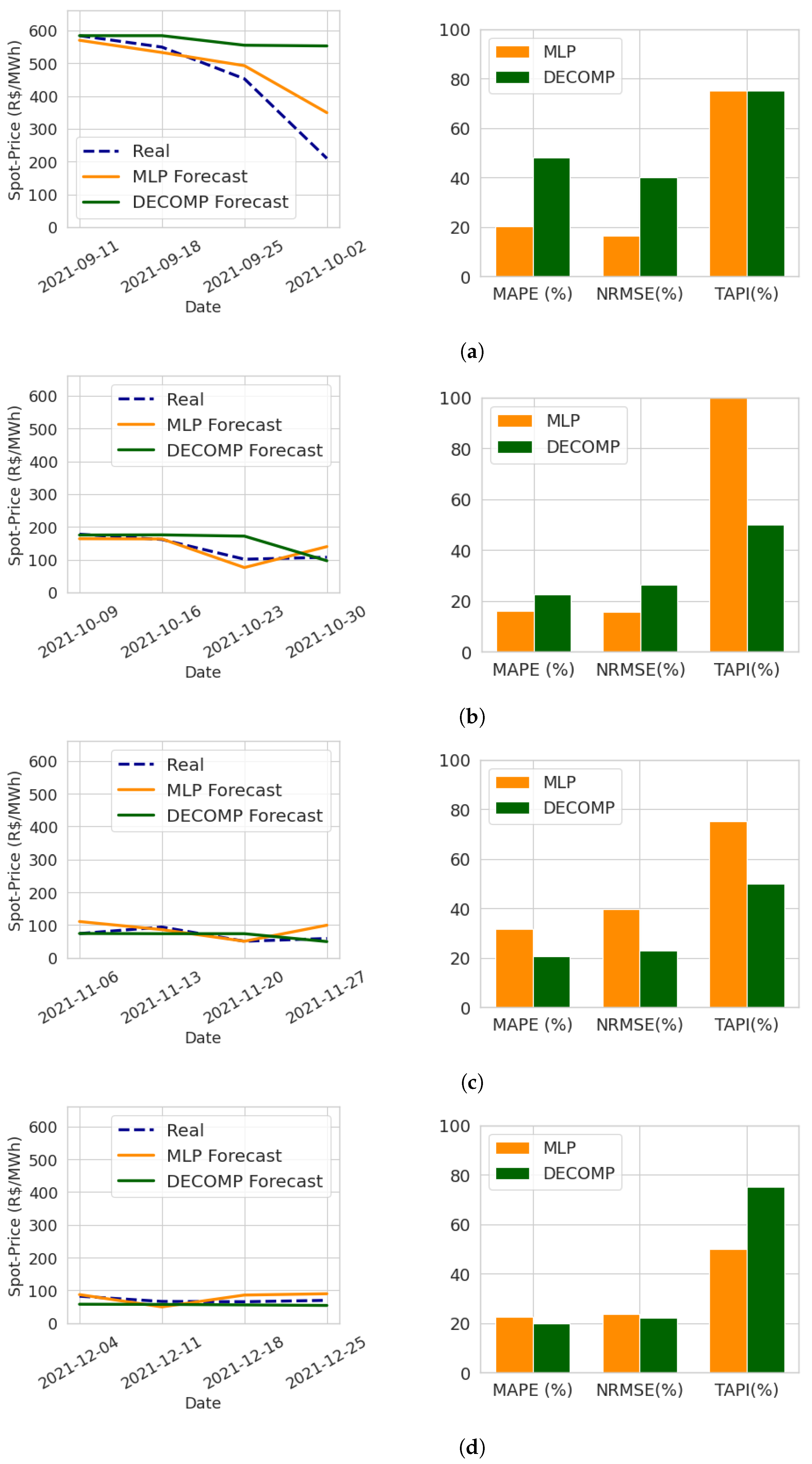
Figure 10 illustrates the comparative performance of the proposed model and the DECOMP model for multi-step forecasting using the test data for the year 2021, as defined by the cross-validation process.

The results obtained throughout 2021 showed that the MLP model achieved better accuracy for trend forecasting during the observation period compared to DECOMP, as indicated by the TAPI index. Furthermore, in the MLP forecasts, the TAPI never dropped below 50% and reached up to 100% in the second forecasting window, indicating that the model consistently managed to capture the trends of price increases or decreases over the weeks.

It was observed that that the MLP model demonstrated lower error metrics (NRMSE and MAPE) during periods of higher volatility in the spot price of energy. Even during moments of significant price variation, such as in the first and second time windows considered, the MLP model consistently managed to track market trends. For instance, in the first time window, the price per MWh ranged from BRL 583.88 to BRL 209.43 over four weeks, with a sharp decline from the third to the fourth week. During this period, the MLP model’s forecasts exhibited error rates below 20%, and successfully predicted the downward trend in prices, achieving a TAPI of 75% for this validation window.

On the other hand, during periods of more stable prices, such as in the third and fourth validation windows, the DECOMP model’s forecasts showed slightly better performance with slightly lower error rates (NRMSE and MAPE) for these observation windows. However, the DECOMP model failed to anticipate the significant price drop observed in the first validation window.

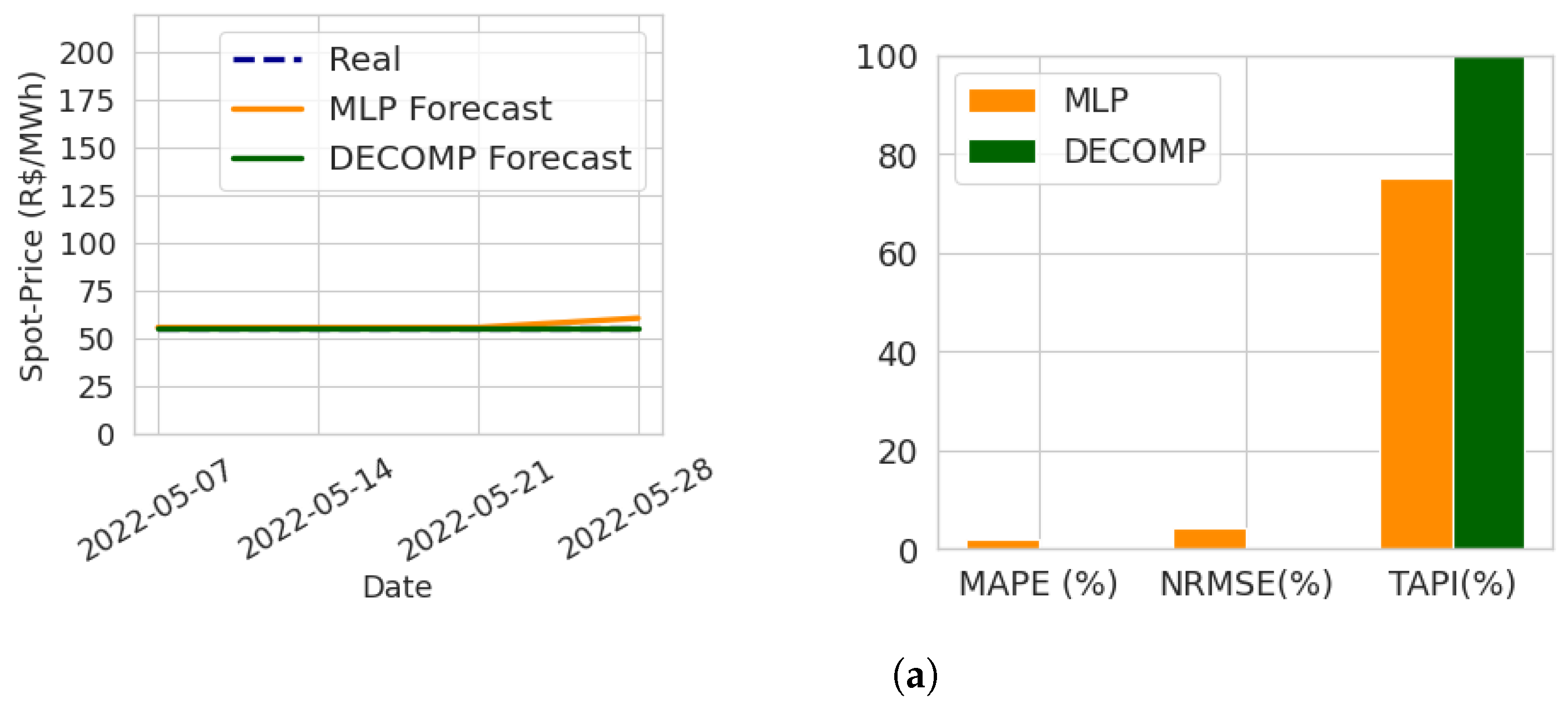
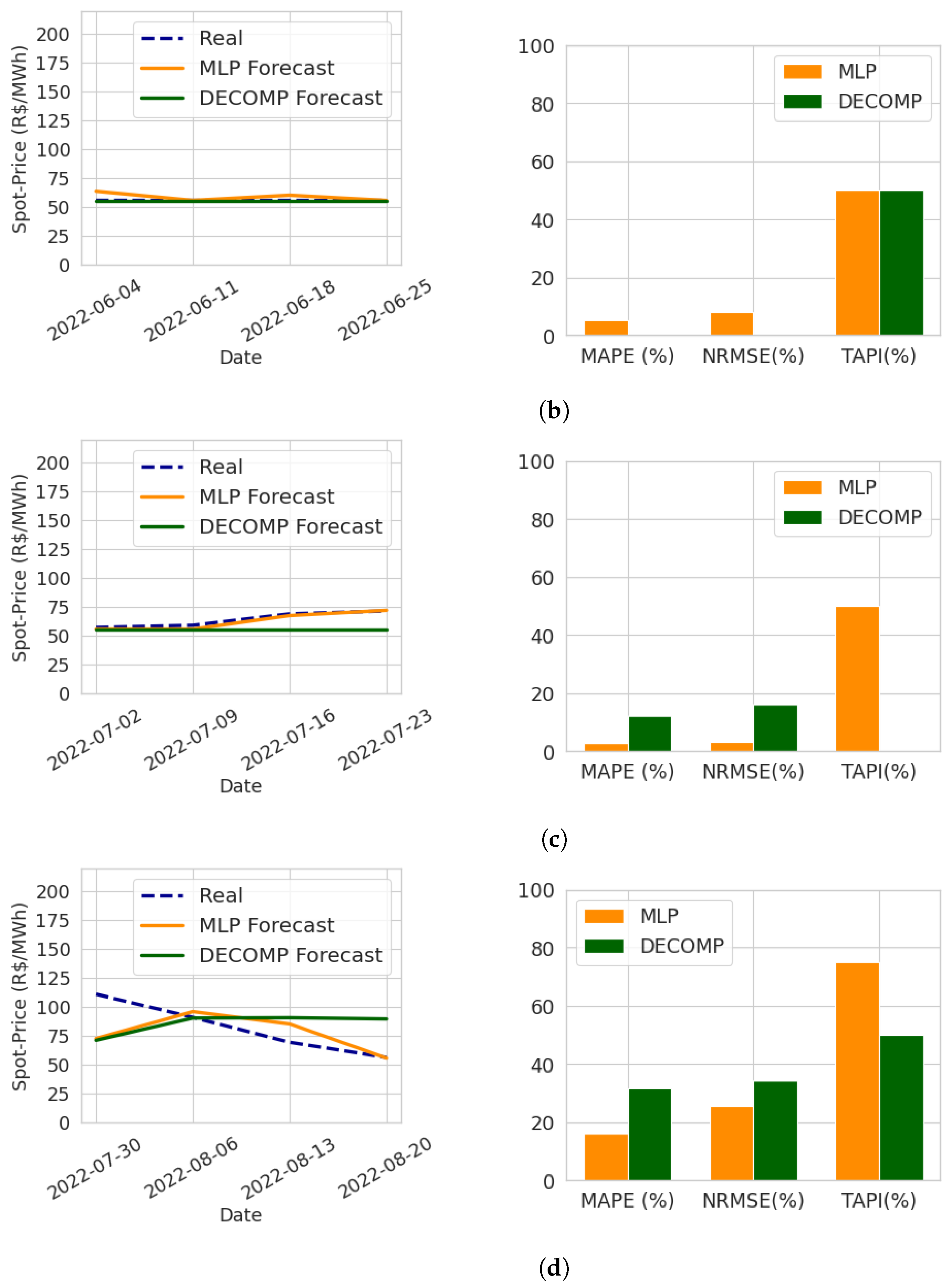
In Figure 11, the performance of the models when projecting prices for the year 2022 is illustrated. Notably, in 2022, the models showed lower error values compared to 2021 for both, due to a smaller price variation.

In the first two validation windows of Figure 11, in which the price barely varied, the DECOMP model demonstrated good performance. However, there was a slight increase in energy prices during the first half of July, followed by a decrease in the second half of July and early August. During this period, the MLP model outperformed, successfully anticipating both the upward and downward trends in energy spot prices.

Regarding the TAPI, similar to observations in the multi-step forecast for 2021, the MLP model stood out, with the indicator consistently remaining equal to or greater than 50% for all forecast horizons. This indicates the model’s ability to generally capture price trends in the Southeast energy market.

Table 2. Models’ performance.

Model	MAPE (%)	NRMSE (%)	TAPI (%)
MLP	14.65	24.70	68.75
DECOMP	19.44	53.89	56.25

provides performance metrics for the models based on spot price predictions for energy in the Southeast region in both 2021 and 2022. Overall, the proposed model exhibited good performance at estimating energy prices, outperforming DECOMP, especially during periods of higher price volatility.

4. Conclusions

This study introduced a methodology for forecasting electricity spot prices in the Brazilian Southeast region using multilayer perceptron as an alternative to the traditional DECOMP model implemented in the country. This model enables the incorporation of additional exogenous variables in addition to the price itself to improve the accuracy of predictions.

Due to the high volatility of energy prices, the model was tested at various time intervals while maintaining a fixed forecasting horizon of four weeks. This approach allowed for the validation of the model’s performance under different market conditions. The results demonstrated the model’s strong performance, with an MAPE of 14.65%, an NRMSE of 24.70%, and a TAPI of 68.75%. Furthermore, the model presented an advantage over the DECOMP model, particularly during periods of greater price volatility.

Strong performance at estimating energy price trends is important for making well-informed decisions in the energy trading sector. If a price increase is anticipated, one can secure an energy contract at the current rates for future resale at a higher price. Conversely, when a price decrease is forecast, it suggests initiating contracts for energy sale under current conditions to be purchased at reduced rates in the future. Through this work, the aim is to support market participants in their decision-making processes related to short-term planning in the energy trading market, allowing them to effectively manage their contract portfolios.