

Reliability-Based Design Optimization of the PEMFC Flow Field with Consideration of Statistical Uncertainty of Design Variables


Abstract
1. Introduction
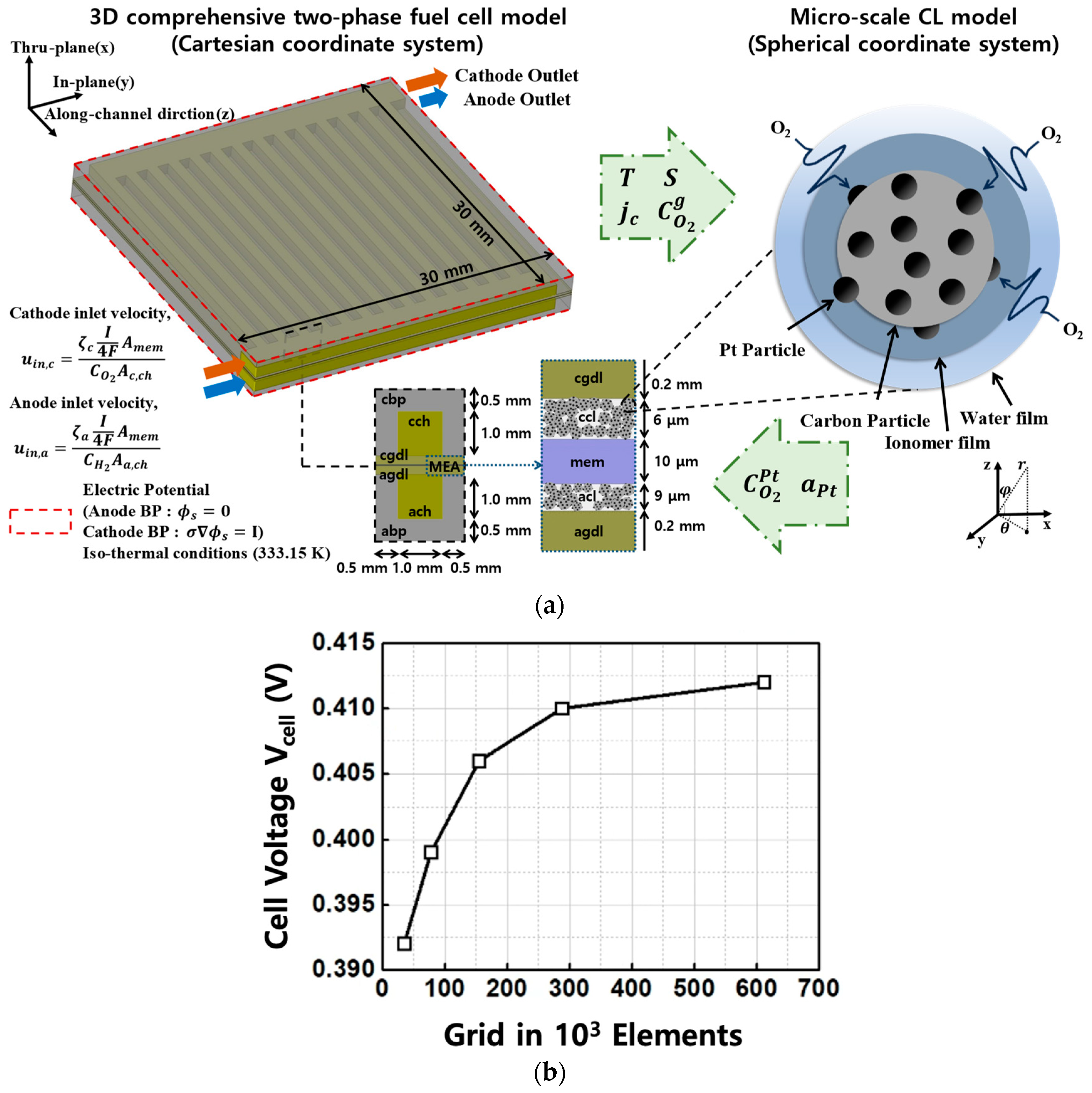
2. Multi-Scale, Multi-Phase 3D PEMFC Model
2.1. Model Assumptions
- (1)
- The present study was guided by a set of specific assumptions outlined below.
- (2)
- Ideal gas mixtures in the gas phase were considered due to the low operating pressures involved.
- (3)
- Flow velocity was assumed to be low, maintaining a laminar condition.
- (4)
- Negligible effects of gravity were taken into account.
- (5)
- The influence of immobile liquid saturation in porous regions was considered to be negligible.
2.2. Governing Equations and Source Terms
2.3. Microscale CL Model
2.4. Boundary Conditions and Numerical Implementation
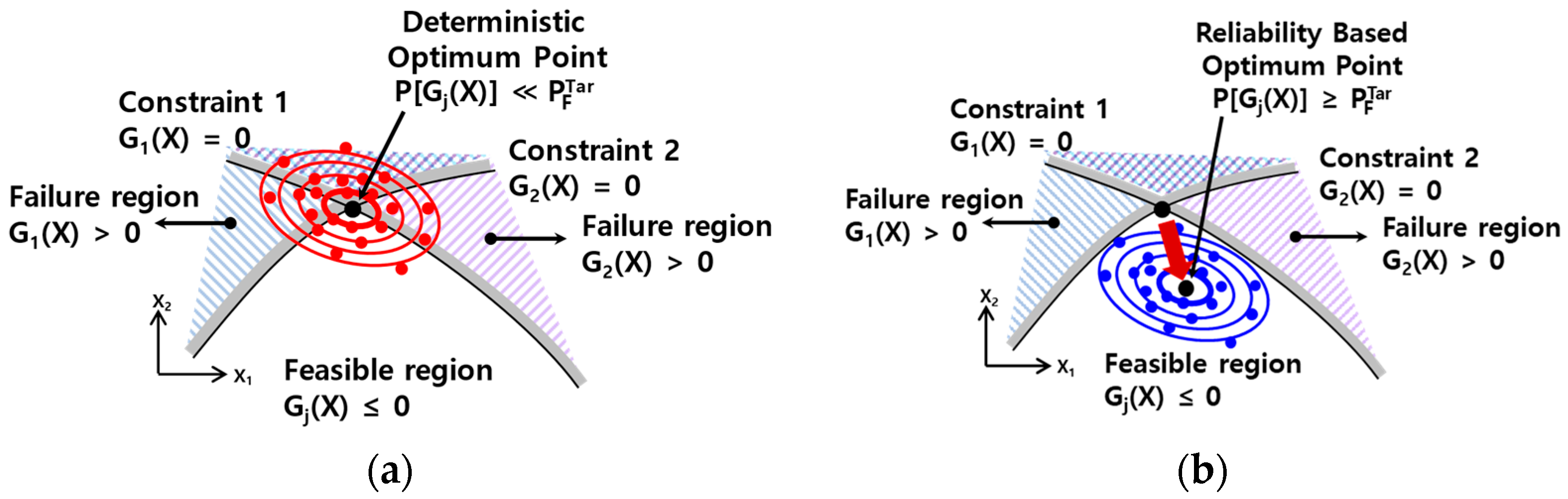
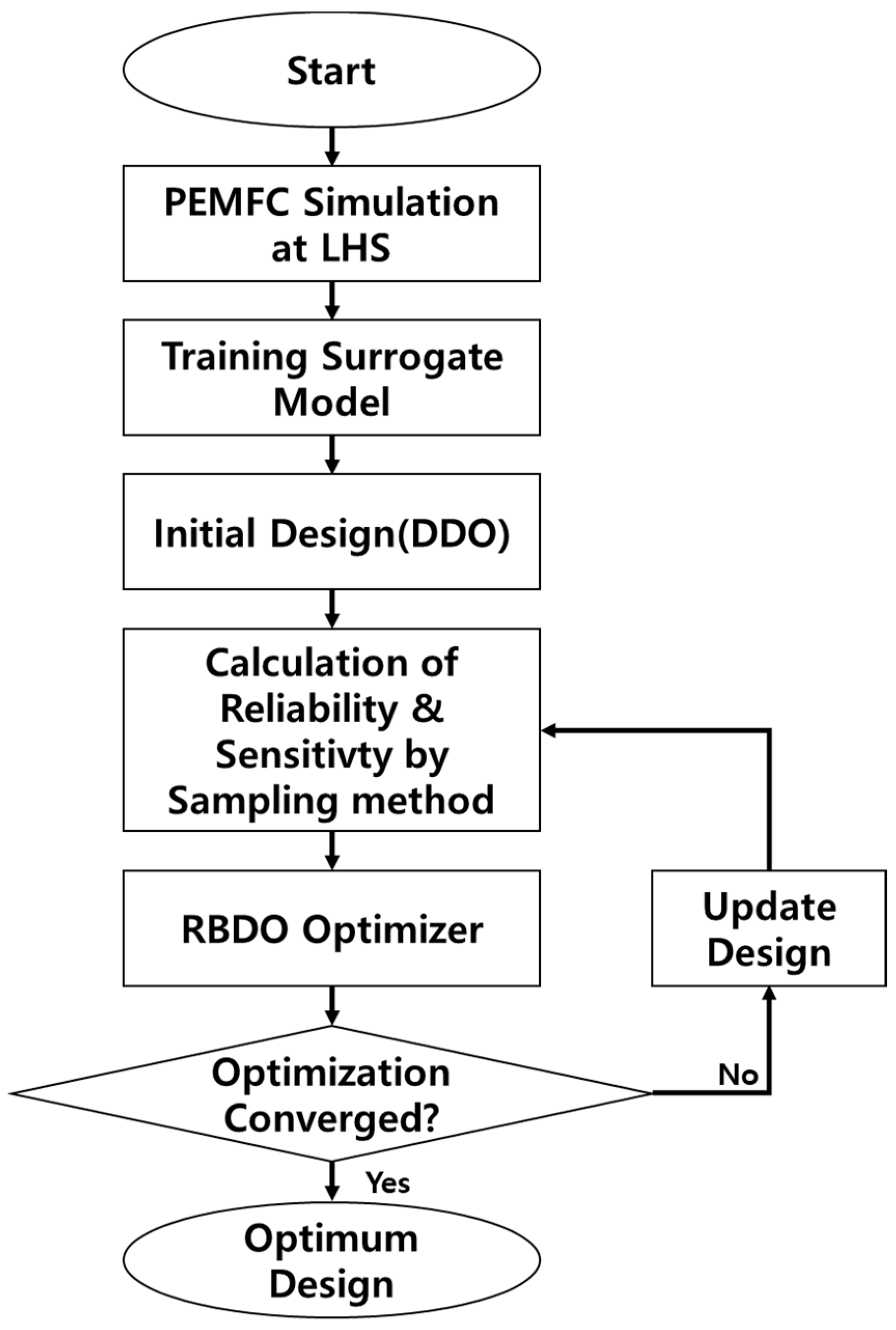
3. Reliability Based Design Optimization
3.1. General Formulation of RBDO
3.2. Sampling-Based RBDO
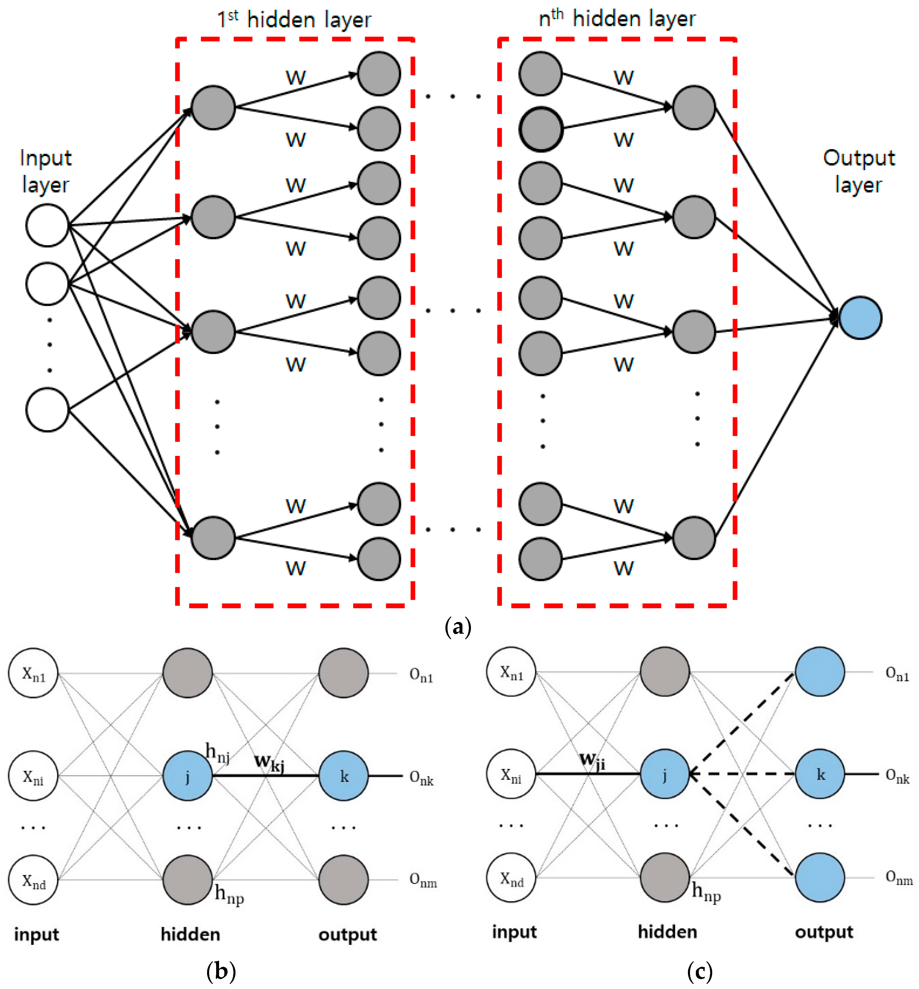
3.3. Metamodeling (Surrogate)
4. Results and Discussion
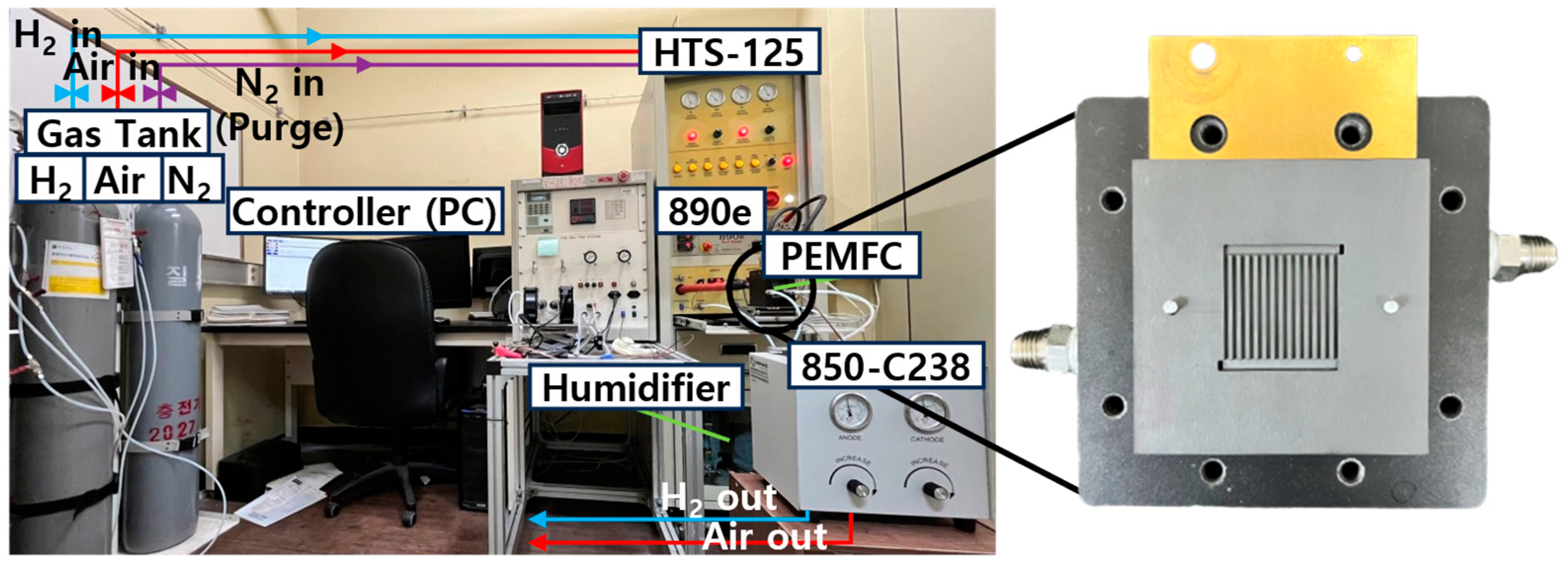
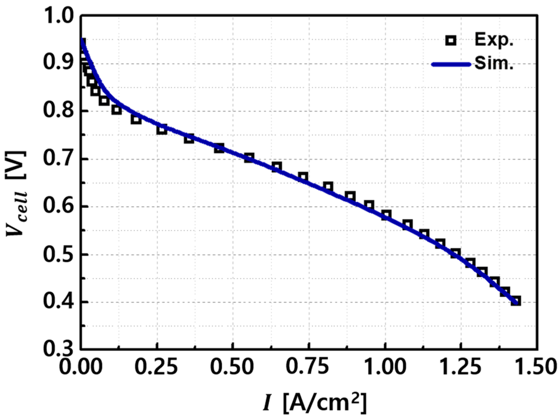
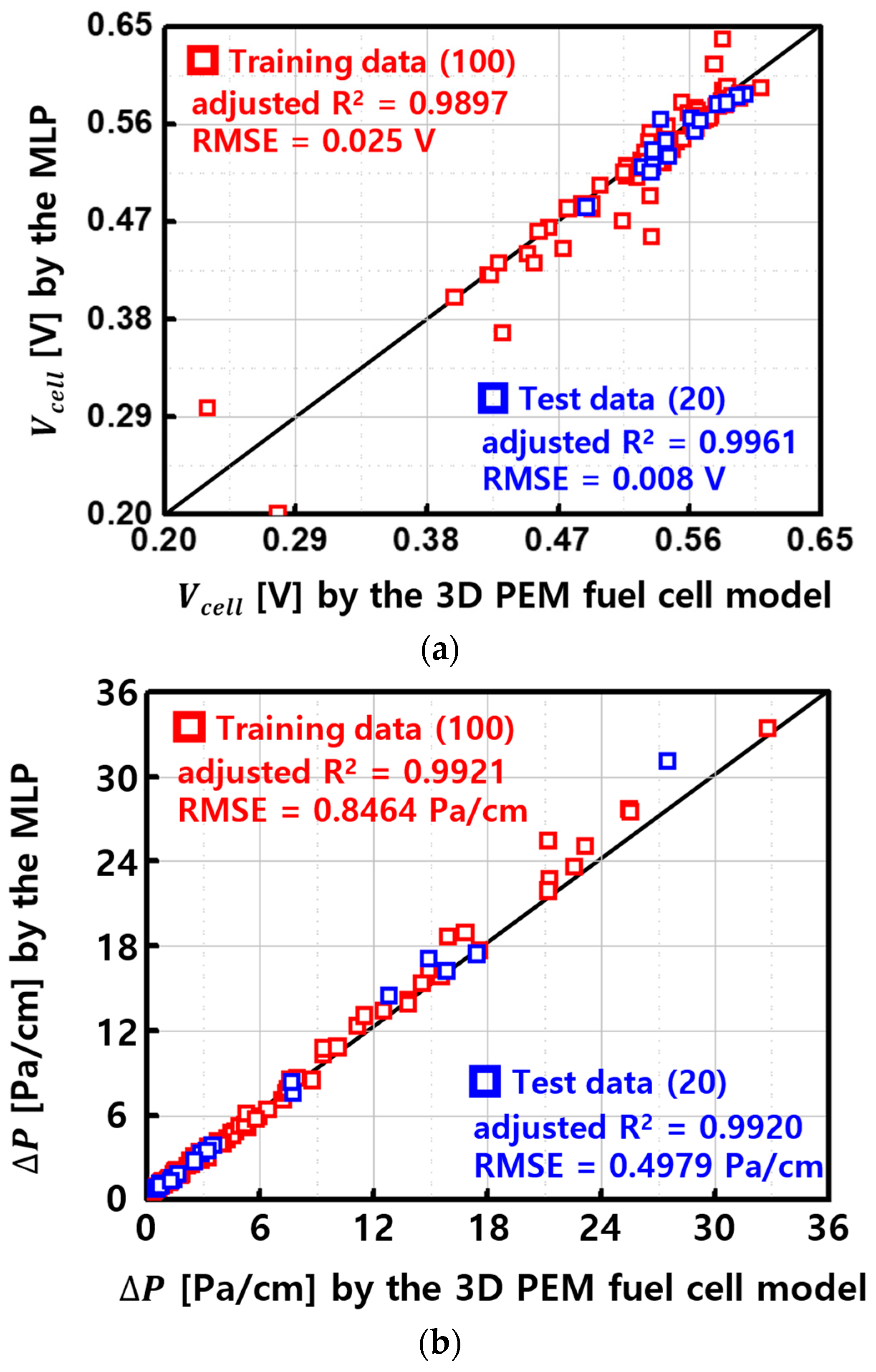
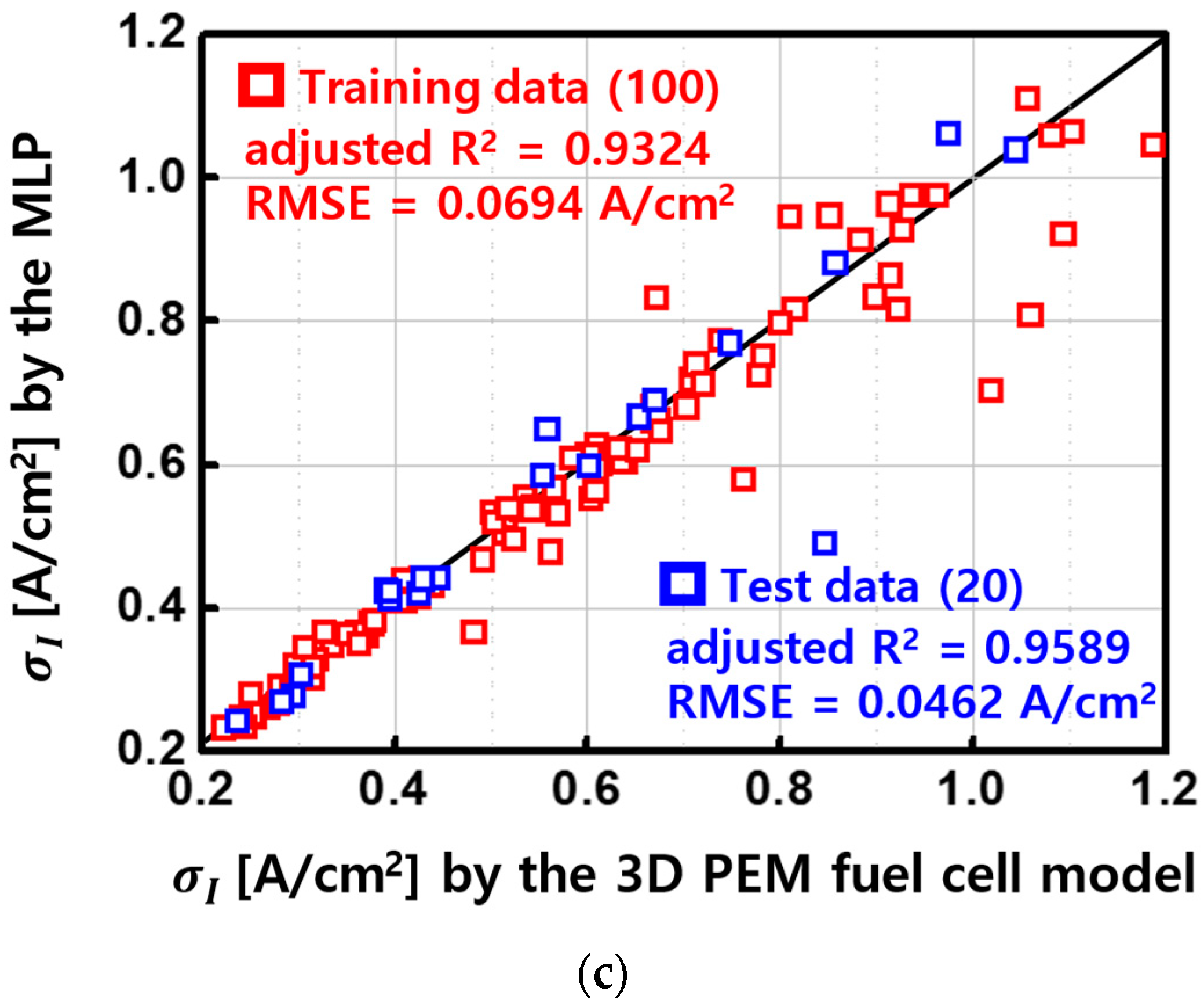
4.1. Experimental Validation of a 3D PEMFC Model and Construction of the MLP Models
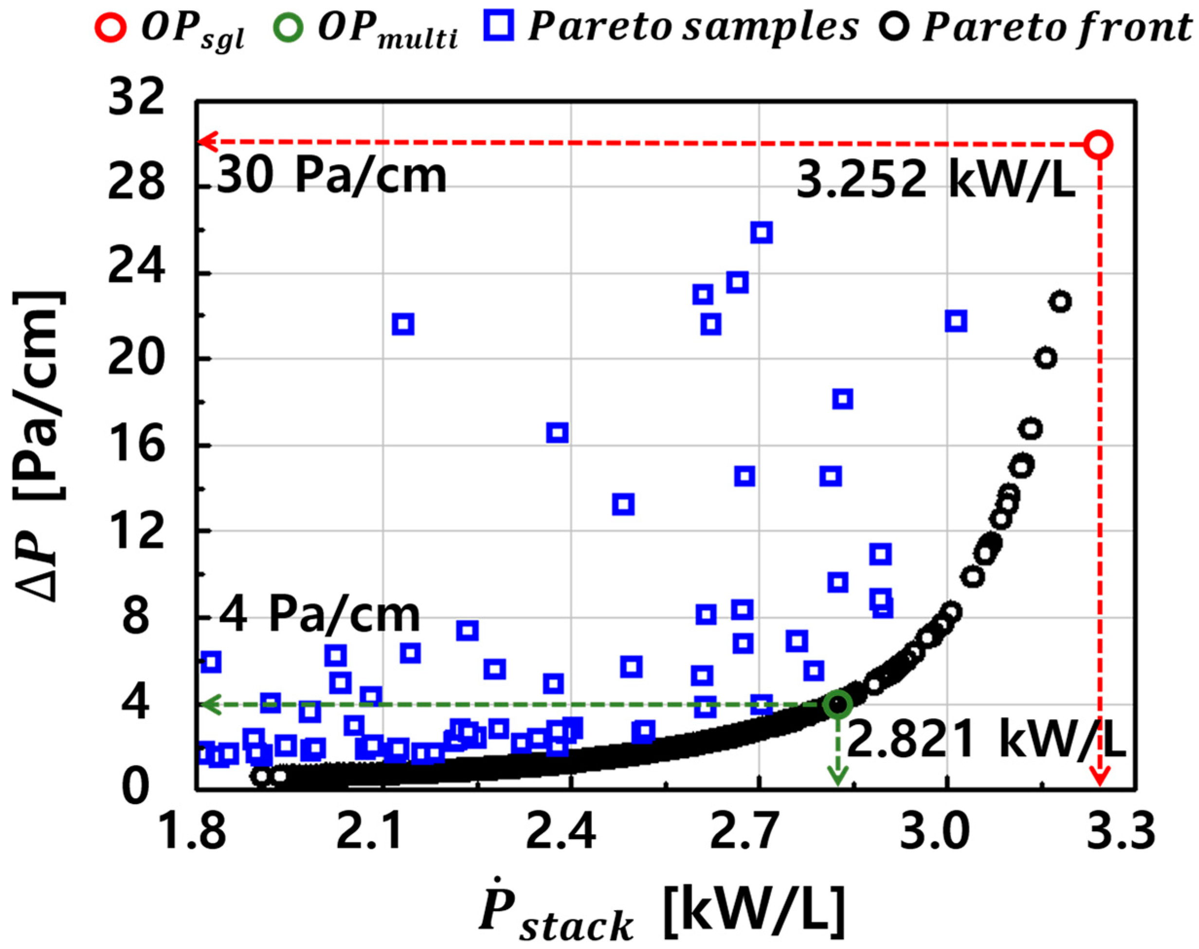
4.2. Comparative Analysis of Single-Objective and Multi-Objective Optimization Methods
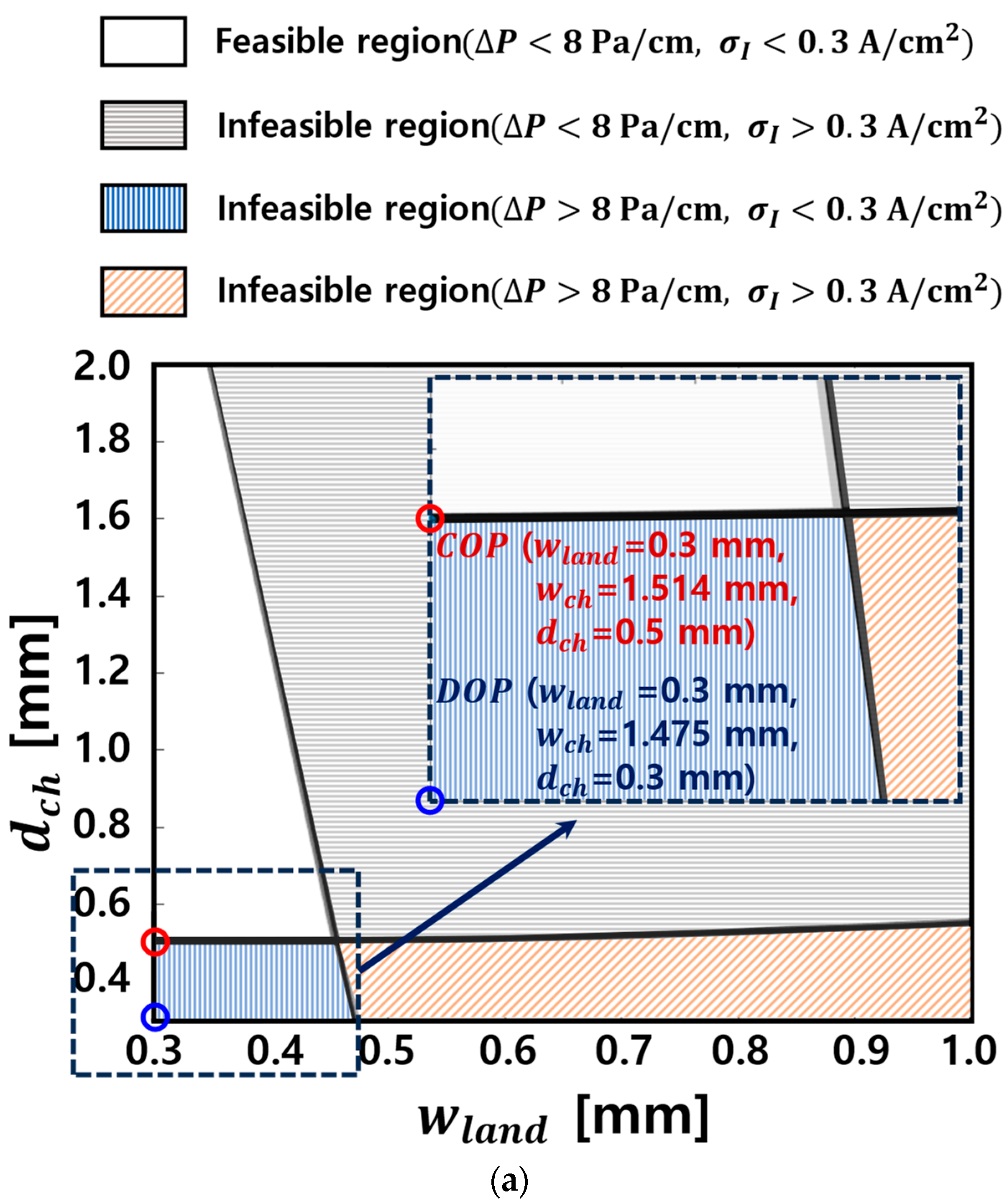
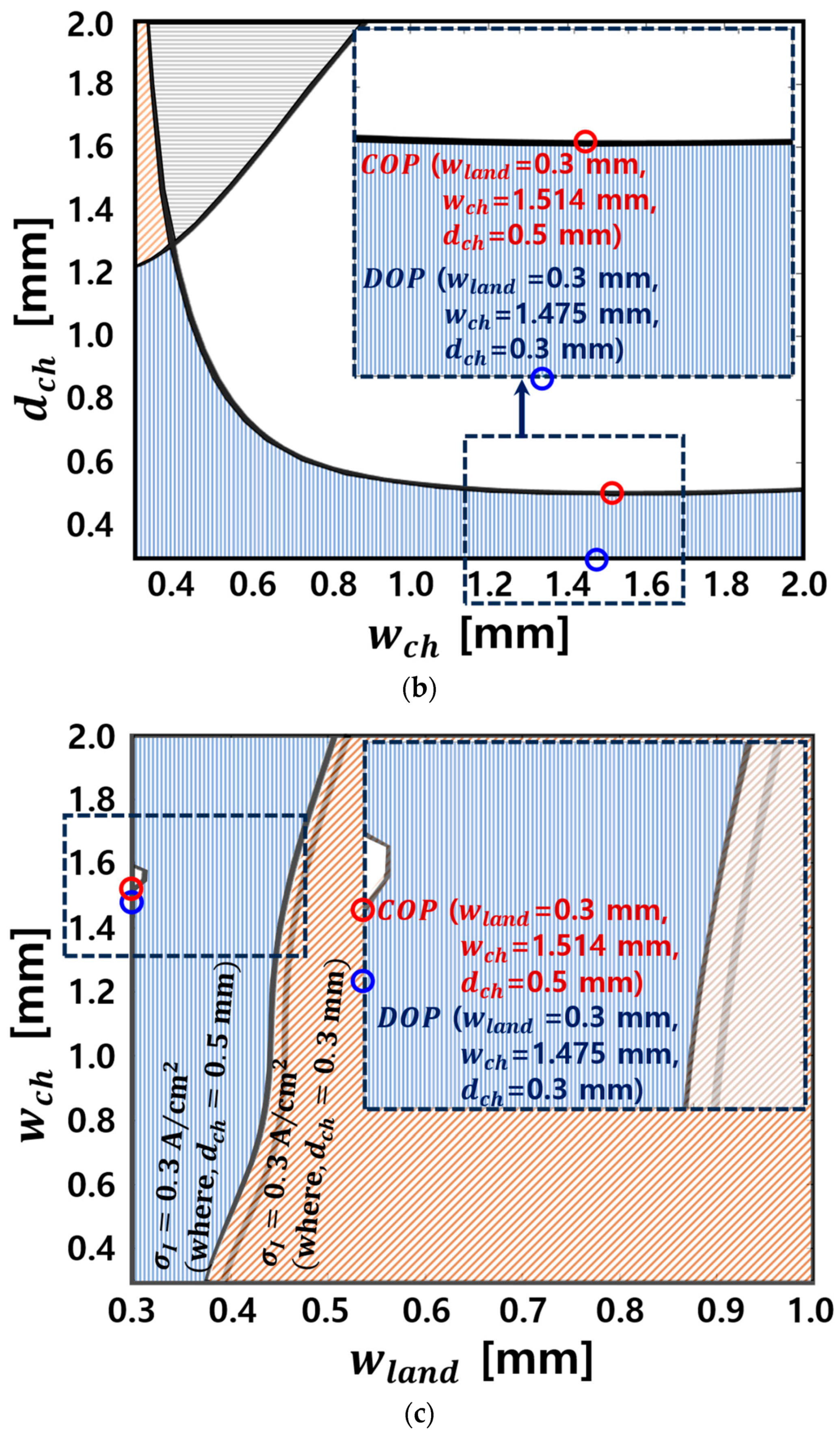
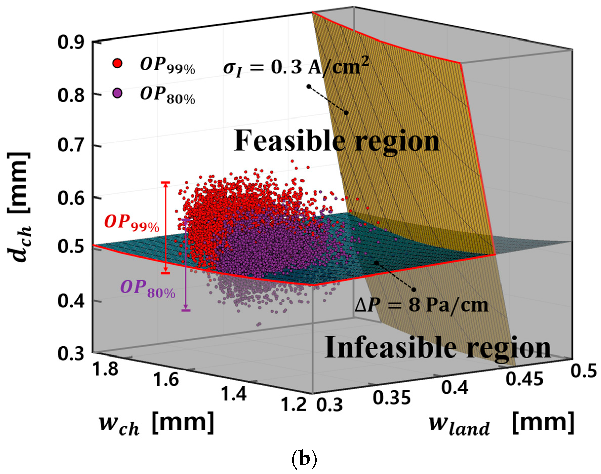
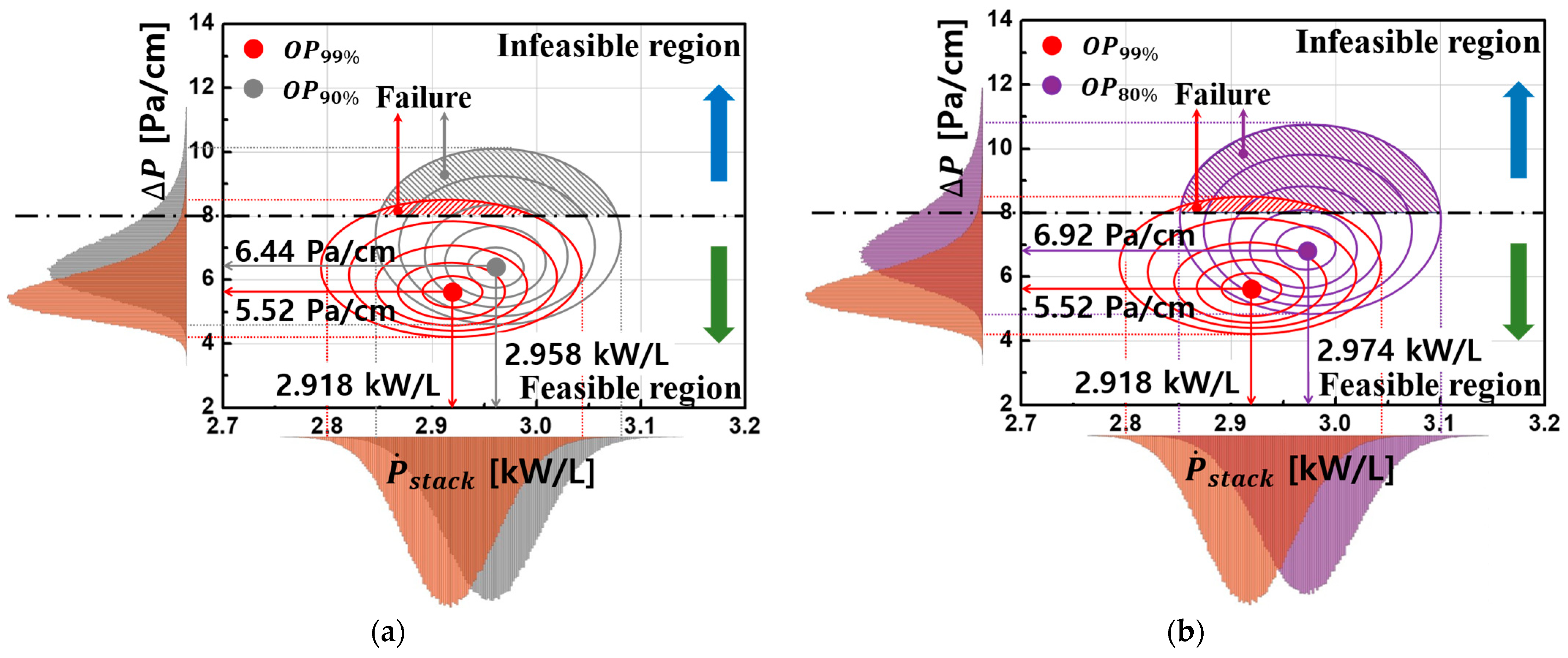
4.3. RBDO Accounting for Output Constraints and Production Tolerances of Design Variables
5. Conclusions
Author Contributions
Funding
Data Availability Statement
Conflicts of Interest
Nomenclature
| a | Ratio of active surface area per unit electrode volume, m2/m3 or water activity | |
| A | Area, m2 | |
| C | Molar concentration of species, mol/m3 or capability | |
| COP | Constrained optimal point | |
| D | Species diffusivity, m2/s | |
| DOP | Deterministic optimal point | |
| d | Diameter or vector of design variables or number of input variables or depth | |
| E | Activation energy, kJ/mol or expectation operator | |
| EW | Equivalent weight of a dry membrane, kg/mol | |
| F | Faraday’s constant, 96,487 C/mol | |
| f | Objective function | |
| G | Global best or deterministic constraint function | |
| H | Joint cumulative density function | |
| h | Joint probability density function or output of the | |
| hidden layer upon activation | ||
| i0 | Exchange current density, A/cm2 | |
| I | Operating current density, A/cm2 or indicator function | |
| j | Transfer current density, A/cm3 | |
| k | Thermal conductivity, W/m·K or relative permeability | |
| K | Hydraulic permeability, m2 | |
| M | Number of Monte Carlo samples | |
| MW | Molecular weight, kg/mol | |
| N | Number of training points | |
| n | Number of electrons transferred in the electrode reaction | |
| nc | Number of probabilistic constraints | |
| nd | Number of design variables | |
| net | Product of weights and the training data | |
| nr | Number of random variables | |
| OP | Optimal point | |
| P | Pressure, Pa | |
| P | Waste product or probability function or power density, kW/L | |
| p | Number of weight coefficients in each second-order equation or number of | |
| weights in the hidden layer | ||
| q | Interpolation coefficient | |
| R | Real space | |
| s | Liquid saturation or the first-order score function | |
| S | Source term in the transport equation | |
| T | Temperature, K | |
| u | Concentration of chemical species U | |
| Fluid velocity and superficial velocity in a porous medium, m/s | ||
| V | Voltage | |
| v | Concentration of chemical species V | |
| W | Matrix of weights | |
| w | Width or weight | |
| wt | Weight ratio | |
| X | Vector of random variables or matrix of design variables | |
| X | Random variable | |
| x | Input variable | |
| z | Transport resistance coefficient | |
| Greek symbols | ||
| α | Transfer coefficient | |
| γ | Reaction order or local density | |
| δ | Thickness, m | |
| ε | Volume fraction | |
| η | Surface overpotential, V | |
| Contact angle of the gas diffusion layer | ||
| κ | Proton conductivity, S/m | |
| Water content | ||
| Mean | ||
| ξ | Stoichiometry flow ratio | |
| ρ | Density, kg/m | |
| σ | Electronic conductivity, S/m or standard deviation | |
| τ | Viscous shear stress, N/m2 | |
| Standard normal cumulative density function or phase potential | ||
| Ω | Oxygen transport resistance | |
| Ω | Failure set | |
| Superscripts | ||
| c | Catalyst coverage coefficient | |
| eff | Effective | |
| g | Gas | |
| l | Liquid | |
| mem | Membrane | |
| ref | Reference value | |
| Tar | Target | |
| Subscripts | ||
| a | Anode | |
| C | Carbon | |
| CL | Catalyst layer | |
| c | Cathode | |
| cell | Cell | |
| ch | Gas channel | |
| e | Electrolyte | |
| F | Failure | |
| gdl | Gas diffusion layer | |
| I | Current density | |
| i | Species or ith random variables | |
| in | Channel inlet | |
| int | Interface | |
| j | jth constraint | |
| k | kth objective function | |
| L | Lower | |
| land | Land | |
| mem | Membrane | |
| multi | Multi objective optimization | |
| p | Process | |
| s | Solid or Surface | |
| sgl | Single objective optimization | |
| stack | Stack | |
| T | Temperature | |
| U | Upper | |
| u | Momentum equation | |
| w | Water | |
| 0 | Initial conditions or standard conditions, i.e., 298.15 K and 101.3 kPa (1 atm) | |
References
- Momirlan, M.; Veziroglu, T.N. Current status of hydrogen energy. Renew. Sustain. Energy Rev. 2002, 6, 141–179. [Google Scholar] [CrossRef]
- Barbir, F. PEM Fuel Cells: Theory and Practice; Academic Press: Cambridge, MA, USA, 2005. [Google Scholar]
- Bernay, C.; Marchand, M.; Cassir, M. Prospects of different fuel cell technologies for vehicle applications. J. Power Sources 2002, 108, 139–152. [Google Scholar] [CrossRef]
- Kirubakaran, A.; Jain, S.; Nema, R.K. A review on fuel cell technologies and power electronic interface. Renew. Sustain. Energy Rev. 2009, 13, 2430–2440. [Google Scholar] [CrossRef]
- Li, X.; Sabir, I. Review of bipolar plates in PEM fuel cells: Flow-field designs. Int. J. Hydrogen Energy 2005, 30, 359–371. [Google Scholar] [CrossRef]
- Ozen, N.D.; Timurkutluk, B.; Altinisik, K. Effects of operation temperature and reactant gas humidity levels on performance of PEM fuel cells. Renew. Sustain. Energy Rev. 2016, 59, 1298–1306. [Google Scholar] [CrossRef]
- Ko, D.; Doh, S.; Park, H.S.; Kim, M.H. Investigation of the effect of operating pressure on the performance of proton exchange membrane fuel cell: In the aspect of water distribution. Renew. Energy 2018, 115, 896–907. [Google Scholar] [CrossRef]
- Gasteiger, H.A.; Yan, S.G. Dependence of PEM fuel cell performance on catalyst loading. J. Power Sources 2004, 127, 162–171. [Google Scholar] [CrossRef]
- Akhtar, N.; Qureshi, A.; Scholta, J.; Hartnig, C.; Messerschmidt, M.; Lehnert, W. Investigation of water droplet kinetics and optimization of channel geometry for PEM fuel cell cathodes. Int. J. Hydrogen Energy 2009, 34, 3104–3111. [Google Scholar] [CrossRef]
- Wang, X.D.; Zhang, X.X.; Yan, W.M.; Lee, D.J.; Su, A. Determination of the optimal active area for proton exchange membrane fuel cells with parallel, interdigitated or serpentine designs. Int. J. Hydrogen Energy 2009, 34, 3823–3832. [Google Scholar] [CrossRef]
- Rao, S. Engineering Optimization: Theory and Practice; John Wiley & Sons: Hoboken, NJ, USA, 2019. [Google Scholar]
- Ye, M.; Wang, X.; Xu, Y. Parameter identification for proton exchange membrane fuel cell model using particle swarm optimization. Int. J. Hydrogen Energy 2009, 34, 981–989. [Google Scholar] [CrossRef]
- Cai, G.; Liang, Y.; Liu, Z.; Liu, W. Design and optimization of bio-inspired wave-like channel for a PEM fuel cell applying genetic algorithm. Energy 2020, 192, 116670. [Google Scholar] [CrossRef]
- Tirnovan, R.; Giurgea, S.; Miraoui, A.; Cirrincione, M. Surrogate model for proton exchange membrane fuel cell (PEMFC). J. Power Sources 2008, 175, 773–778. [Google Scholar] [CrossRef]
- Tirnovan, R.; Giurgea, S.; Miraoui, A.; Cirrincione, M. Surrogate modelling of compressor characteristics for fuel-cell applications. Appl. Energy 2008, 85, 394–403. [Google Scholar] [CrossRef]
- Forrester, A.I.; Keane, A.J. Recent advances in surrogate-based optimization. Prog. Aerosp. Sci. 2009, 45, 50–79. [Google Scholar] [CrossRef]
- Choi, J.; Cha, Y.; Kong, J.; Vaz, N.; Lee, J.; Ma, S.-B.; Kim, J.-H.; Lee, S.W.; Jang, S.S.; Ju, H. Multi-Variate Optimization of Polymer Electrolyte Membrane Fuel Cells in Consideration of Effects of GDL Compression and Intrusion. J. Electrochem. Soc. 2022, 169, 14511. [Google Scholar] [CrossRef]
- Zhang, G.; Wu, L.; Jiao, K.; Tian, P.; Wang, B.; Wang, Y.; Liu, Z. Optimization of porous media flow field for proton exchange membrane fuel cell using a data-driven surrogate model. Energy Convers. Manag. 2020, 226, 113513. [Google Scholar] [CrossRef]
- Bauer, F.; Denneler, S.; Willert-Porada, M. Influence of temperature and humidity on the mechanical properties of Nafion® 117 polymer electrolyte membrane. J. Polym. Sci. Part B Polym. Phys. 2005, 43, 786–795. [Google Scholar] [CrossRef]
- Lamberti, L.; Pappalettere, C. Comparison of the numerical efficiency of different sequential linear programming based algorithms for structural optimisation problems. Comput. Struct. 2000, 76, 713–728. [Google Scholar] [CrossRef]
- Antoniou, A.; Lu, W.S. Optimization: Methods, Algorithms, and Applications; Kluwer Academic: New York, NY, USA, 2003. [Google Scholar]
- Tu, J.; Choi, K.K.; Park, Y.H. A new study on reliability-based design optimization. J. Mech. Des. 1999, 121, 557–564. [Google Scholar] [CrossRef]
- Enevoldsen, I.; Sørensen, J.D. Reliability-based optimization in structural engineering. Struct. Saf. 1994, 15, 169–196. [Google Scholar] [CrossRef]
- Chandu, S.V.; Grandhi, R.V. General purpose procedure for reliability based structural optimization under parametric uncertainties. Adv. Eng. Softw. 1995, 23, 7–14. [Google Scholar] [CrossRef]
- Mun, J.; Lim, J.; Kwak, Y.; Kang, B.; Choi, K.K.; Kim, D.H. Reliability-based design optimization of a permanent magnet motor under manufacturing tolerance and temperature fluctuation. IEEE Trans. Magn. 2021, 57, 8203304. [Google Scholar] [CrossRef]
- Youn, B.D.; Choi, K.K.; Park, Y.H. Hybrid analysis method for reliability-based design optimization. J. Mech. Des. 2003, 125, 221–232. [Google Scholar] [CrossRef]
- Zeng, Y.; Li, Y.F.; Li, X.Y.; Huang, H.Z. Tolerance-based reliability and optimization design of switched-mode power supply. Qual. Reliab. Eng. Int. 2019, 35, 2774–2784. [Google Scholar] [CrossRef]
- Wang, Y.; Basu, S.; Wang, C.-Y. Modeling two-phase flow in PEM fuel cell channels. J. Power Sources 2008, 179, 603–617. [Google Scholar] [CrossRef]
- Jo, A.; Ju, H. Numerical study on applicability of metal foam as flow distributor in polymer electrolyte fuel cells (PEFCs). Int. J. Hydrog. Energy 2018, 43, 14012–14026. [Google Scholar] [CrossRef]
- Choi, K.K.; Youn, B.D. Reliability-Based Design Optimization of Structural Durability Under Manufacturing Tolerances. In Proceedings of the Fifth World Congress of Structural and Multidisciplinary Optimization, Lido di Jesolo-Venice, Italy, 19–23 May 2003. [Google Scholar]
- Au, S.-K.; Beck, J.L. Estimation of small failure probabilities in high dimensions by subset simulation. Probabilistic Eng. Mech. 2001, 16, 263–277. [Google Scholar] [CrossRef]
- Haldar, A.; Mahadevan, S. Probability, Reliability and Statistical Methods in Engineering Design; Wiley: Hoboken, NJ, USA, 2000. [Google Scholar]
- Hohenbichler, M.; Rackwitz, R. Improvement of second-order reliability estimates by importance sampling. J. Eng. Mech. 1988, 114, 2195–2199. [Google Scholar] [CrossRef]
- Zeeb, C.N.; Burns, P.J.; Collins, F. A Comparison of Failure Probability Estimates by Monte Carlo Sampling and Latin Hypercube Sampling; Sandia National Laboratories: Livermore, CA, USA, 1998. [Google Scholar]
- Park, J.W.; Lee, I. A new framework for efficient sequential sampling-based RBDO using space mapping. J. Mech. Des. 2023, 145, 31702. [Google Scholar] [CrossRef]
- Tsompanakis, Y.; Papadrakakis, M. Large-scale reliability-based structural optimization. Struct. Multidiscip. Optim. 2004, 26, 429–440. [Google Scholar] [CrossRef]
- Lee, I.; Choi, K.K.; Noh, Y.; Zhao, L.; Gorsich, D. Sampling-based stochastic sensitivity analysis using score functions for RBDO problems with correlated random variables. J. Mech. Des. 2011, 133, 021003. [Google Scholar] [CrossRef]
- Valdebenito, M.A.; Schuëller, G.I. A survey on approaches for reliability-based optimization. Struct. Multidiscip. Optim. 2010, 42, 645–663. [Google Scholar] [CrossRef]
- Youn, B.D.; Choi, K.K. A new response surface methodology for reliability-based design optimization. Comput. Struct. 2004, 82, 241–256. [Google Scholar] [CrossRef]
- Vaz, N.; Choi, J.; Cha, Y.; Kong, J.; Park, Y.; Ju, H. Multi-objective optimization of the cathode catalyst layer micro-composition of polymer electrolyte membrane fuel cells using a multi-scale, two-phase fuel cell model and data-driven surrogates. J. Energy Chem. 2023, 81, 28–41. [Google Scholar] [CrossRef]
- Kiran, D.R. Total Quality Management: Key Concepts and Case Studies; Butterworth-Heinemann: Oxford, UK, 2016. [Google Scholar]
- Stepanova, V.; Erins, I. ICT Transfer Business Model Development. Int. J. Mach. Learn. Comput. 2020, 10, 170–175. [Google Scholar] [CrossRef]


| Governing Equations | ||
|---|---|---|
| Mass | (1) | |
| Momentum | (2) | |
| Species | Flow channels and porous media: | (3) |
| Water transport in membrane: | (4) | |
| Charge | Proton transport: | (5) |
| Electron transport: | (6) | |
| Energy | (7) | |
| Description | Expression | ||
|---|---|---|---|
| Momentum | Porous media | ||
| Species | H2 in anode CL | ||
| O2 in cathode CL | |||
| Water in anode CL | |||
| Water in cathode CL | |||
| Energy | In anode CL | ||
| In cathode CL | |||
| In membrane | |||
| Charge | In CLs: | ||
| Electrochemical reactions HOR on the anode side: ORR on the cathode side: | |||
| Transfer current density, | HOR in anode CL: | (8) | |
| ORR in cathode CL: | (9) | ||
| Overpotential | where | (10) | |
| Description | Value/Expression | Ref. |
|---|---|---|
| Activation energy of anode, | 10.0 kJ/mol | [24] |
| Activation energy of cathode, | 70.0 kJ/mol | [24] |
| Transfer coefficient of HOR, | 1 | [28] |
| Transfer coefficient of ORR, | 1 | [28] |
| Reference H2/O2 molar concentration, | 40.88 mol/m3 | [28] |
| Permeability of GDL/CL, | 1.0 × 10⁻¹²/1.0 × 10−13 m2 | [24] |
| Equivalent weight of electrolyte in the membrane, | 1.1 kg/mol | [24] |
| Faraday’s constant, | 96,485 C/mol | [28] |
| Universal gas constant, | 8.314 | |
| H2 diffusivity in the anode gas channel, | 1.1028 × 10⁻⁴ m2/s | [28] |
| H2O diffusivity in the anode gas channel, | 1.1028 × 10⁻⁴ m2/s | [28] |
| O2 diffusivity in the cathode gas channel, | 3.2348 × 10⁻⁴ m2/s | [28] |
| H2O diffusivity in the cathode gas channel, | 7.35 × 10⁻⁵ m2/s | [28] |
| Binary gas diffusivity ( | For nonporous regions | (11) |
| Effective diffusivity ( | For porous regions | (12) |
| Description | Expression | |
|---|---|---|
| Mixture density ( | (13) | |
| Gas mixture density | (14) | |
| Mixture velocity ( | (15) | |
| Mixture mass fraction | (16) | |
| Relative permeability | (17) | |
| (18) | ||
| Kinematic viscosity of the two-phase mixture | (19) | |
| Kinematic viscosity of the gas mixture | (20) | |
| where and | (21) | |
| , T in kelvin | (22) | |
| Relative mobility | (23) | |
| (24) | ||
| Diffusive mass flux | (25) | |
| Capillary pressure Pc | (26) | |
| Leverett function J(s) | (27) |
| Description | Expression | |
|---|---|---|
| Membrane water content (λ) | Water | (28) |
| Water activity, | (29) | |
| Electro-osmotic drag (EOD) coefficient of water | (30) | |
| Proton conductivity () | (31) | |
| Water diffusion coefficient () | (32) | |
| Interfacial resistance of the water film | (33) |
| Description | Expression | |
|---|---|---|
| Carbon volume fraction () | (34) | |
| Pt particle volume fraction () | (35) | |
| Ionomer volume fraction () | (36) | |
| CL thickness () | (37) | |
| Thickness of the ionomer film () | (38) | |
| Thickness of water film () | (39) | |
| Oxygen balance in a single Pt/C particle domain | (40) | |
| Volumetric surface area of ionomer ( | (41) | |
| Volumetric surface area of Pt ( | (42) | |
| (43) | ||
| Total oxygen transport resistance ( | (44) | |
| Total transport resistance | (45a) | |
| Interfacial resistance in ionomer | (45b) | |
| Interfacial resistance in water film | (45c) | |
| Interfacial resistance in platinum particle | (45d) | |
| Effective ionomer thickness | (46) | |
| Effective water thickness | (47) | |
| Number of Pt particles on a single carbon particle | (48) | |
| Oxygen concentration on the Pt particle surfaces | (49) |
| Description | Expression | |
|---|---|---|
| Anode inlet velocity | (50) | |
| Cathode inlet velocity | (51) | |
| Constant temperature on side walls | (52) | |
| Heat flux on the top and bottom surfaces | (53) | |
| Electric potential on anode outer BP surface | (54) | |
| Electric potential on cathode outer BP surface | (55) | |
| Pressure(anode/cathode), | 2/2 bar | |
| Operating temperature, | 333.15 K | |
| Stoichiometry(anode/cathode), | 1.5/2.0 |
| Design Cases | Design Variables | [kW/L] | [Pa/cm] | Reliability | |||
|---|---|---|---|---|---|---|---|
[mm] | [mm] | [mm] | PG1 [%] | PG2 [%] | |||
| Ref. point | 1.00 | 1.00 | 1.00 | 1.667 | 2.832 | 100 | 0.00 |
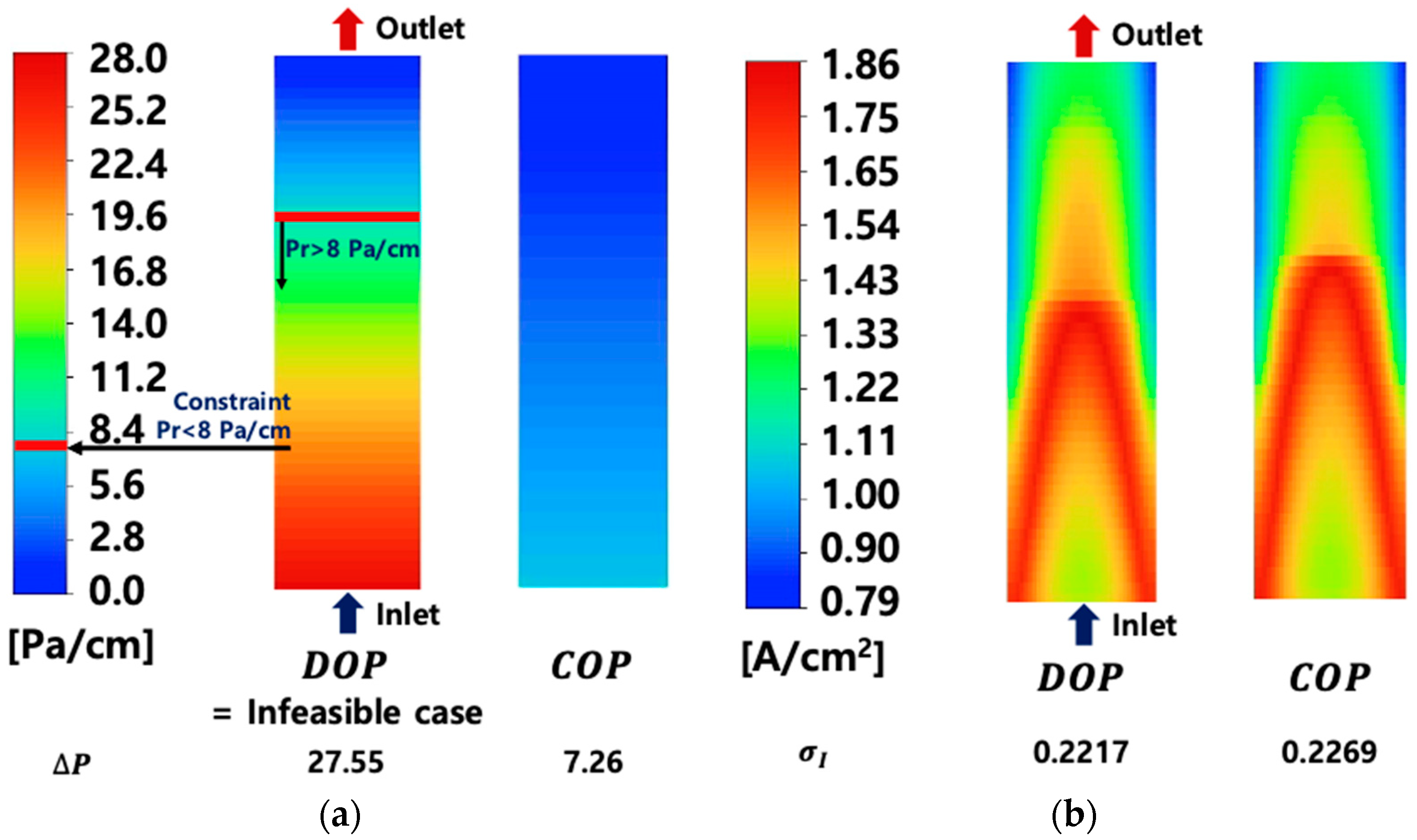
| Deterministic Optimum point (DOP) | 0.30 | 1.48 | 0.30 | 3.252 | 30.209 | 0.00 | 100 |
| Constraint Optimum point (COP) | 0.30 | 1.51 | 0.50 | 3.008 | 8.000 | 49.79 | 100 |
| RBDO | 0.30 | 1.46 | 0.53 | 2.974 | 6.918 | 80.04 | 99.99 |
| RBDO | 0.30 | 1.51 | 0.54 | 2.958 | 6.453 | 90.21 | 99.99 |
| RBDO | 0.30 | 1.55 | 0.58 | 2.918 | 5.519 | 99.13 | 99.99 |
Disclaimer/Publisher’s Note: The statements, opinions and data contained in all publications are solely those of the individual author(s) and contributor(s) and not of MDPI and/or the editor(s). MDPI and/or the editor(s) disclaim responsibility for any injury to people or property resulting from any ideas, methods, instructions or products referred to in the content. |
© 2024 by the authors. Licensee MDPI, Basel, Switzerland. This article is an open access article distributed under the terms and conditions of the Creative Commons Attribution (CC BY) license (https://creativecommons.org/licenses/by/4.0/).
Share and Cite
Heo, S.; Choi, J.; Park, Y.; Vaz, N.; Ju, H. Reliability-Based Design Optimization of the PEMFC Flow Field with Consideration of Statistical Uncertainty of Design Variables. Energies 2024, 17, 1882. https://doi.org/10.3390/en17081882
Heo S, Choi J, Park Y, Vaz N, Ju H. Reliability-Based Design Optimization of the PEMFC Flow Field with Consideration of Statistical Uncertainty of Design Variables. Energies. 2024; 17(8):1882. https://doi.org/10.3390/en17081882
Chicago/Turabian StyleHeo, Seongku, Jaeyoo Choi, Yooseong Park, Neil Vaz, and Hyunchul Ju. 2024. "Reliability-Based Design Optimization of the PEMFC Flow Field with Consideration of Statistical Uncertainty of Design Variables" Energies 17, no. 8: 1882. https://doi.org/10.3390/en17081882
APA StyleHeo, S., Choi, J., Park, Y., Vaz, N., & Ju, H. (2024). Reliability-Based Design Optimization of the PEMFC Flow Field with Consideration of Statistical Uncertainty of Design Variables. Energies, 17(8), 1882. https://doi.org/10.3390/en17081882