Article

Acoustic Design Parameter Change of a Pressurized Combustor Leading to Limit Cycle Oscillations

Faculty of Engineering Technology, University of Twente, 7522 NB Enschede, The Netherlands
*
Author to whom correspondence should be addressed.
Energies 2024, 17(8), 1885; https://doi.org/10.3390/en17081885
Submission received: 21 February 2024 / Revised: 27 March 2024 / Accepted: 12 April 2024 / Published: 15 April 2024
(This article belongs to the Special Issue Heat Transfer and Advanced Combustion in Gas Turbines)

Abstract

:
When aiming to cut down on the emission of nitric oxides by gas turbine engines, it is advantageous to have them operate at low combustion temperatures. This is achieved by lean premixed combustion. Although lean premixed combustion is a proven and promising technology, it is also very sensitive to thermoacoustic instabilities. These instabilities occur due to a coupling between the unsteady heat release rate of the flame and the acoustic field inside the combustion chamber. In this paper, this coupling is investigated in detail. Two acoustic design parameters of a swirl-stabilized pressurized preheated air (300 °C)/natural gas combustor are varied, and the occurrence of thermoacoustic limit cycle oscillations is explored. The sensitivity of the acoustic field as a function of combustion chamber length (0.9 m to 1.8 m) and reflection coefficient (0.7 and 0.9) at the exit of the combustor is investigated first using a hybrid numerical and analytical approach. ANSYS CFX is used for Unsteady Reynolds Averaged Navier-Stokes (URANS) numerical simulations, and a one-dimensional acoustic network model is used for the analytical investigation. Subsequently, the effects of a change in the reflection coefficient are validated on a pressurized combustor test rig at 125 kW and 1.5 bar. With the change in reflection coefficient, the combustor switched to limit cycle oscillation as predicted, and reached a sound pressure level of 150 dB.

1. Introduction

Gas turbine engines are a key technology in industrial and large-scale power and heat generation. To meet future energy challenges, recent innovation in gas turbine technology has been focused on developing more efficient, reliable, and less polluting engines. To cut down the emission of NOX, it is advantageous to operate gas turbine engines at low temperatures. This is achieved by lean premixed combustion, in which the flame temperature is lowered by mixing more air with the fuel than is necessary for stoichiometric oxidation. Although lean premixed combustion of natural gas is a proven and promising technology, it is also very sensitive to thermoacoustic instabilities. These instabilities occur due to a coupling between the unsteady heat release rate of the flame and the acoustic field inside the combustion chamber [1] and can trigger a self-excited oscillation with a high amplitude, leading to a structural failure of the liner.
The principles of combustion instabilities are still not well understood, making it difficult to prepare for all use cases where a given combustor would experience instability [2]. Thus, commissioning a gas turbine becomes a major risk, and may require adjustments to the combustor and/or modifications to the control parameters on site. These adjustments are often expensive in terms of time and money and may hinder the performance of the combustor.
Combustion instability is influenced by intricate physical mechanisms, mostly determined by the system’s geometry and operating conditions [3]. In the literature, thermoacoustic instabilities in many technologies, such as gas turbines, domestic boilers, industrial burners, and propulsion engines, have been investigated [4]. Among these technologies, the combustor featuring a swirl burner stands out as the prevailing design for gas turbine engines due to its ability to maintain high stability limits for most types of flames [5].
Thermoacoustic instabilities are often described by a feedback loop between heat release rate fluctuations, pressure fluctuations, and a coupling mechanism [6]. In order to reach limit cycle oscillations, the energy added to the system by this feedback loop has to be greater than the losses. This feedback loop has received a lot of attention in the literature [7,8]. Some authors (for example, Chen et al. [9]) have studied the interaction of acoustic waves and entropy waves. However, in the current research, the flame front is stationary thanks to the strong anchoring of the swirl stabilized flame, so this approach is not used. Of relevance to the present study, Lee [10] investigated combustion instabilities in a swirler stabilized combustor, where both fuel injection location and combustor length could be varied using a movable plug at the outlet. It was shown that a change in chamber length affected the thermoacoustic properties of the combustor. These results prove that the amplitude and frequency of an instability depend continuously on the length of the combustion chamber. Kim et al. [11] also examined self-excited and forced combustion instabilities by changing the length of the combustor. They used the flame transfer function as the input to their calculating tool in order to anticipate the unstable operation of the combustor. By adjusting the combustor’s length, they were able to find a good agreement between the expected instabilities and self-excitation. Another study by Evesque [12] showed that the pressure amplitude of the natural mode of a Rijke tube is increased by a factor of 1.5 if the length is tuned. Zhang et al. [13] also used variable length combustors with range of 300–1100 mm to investigate thermoacoustic instabilities. They studied the effect of hydrogen addition to methane. Their study showed changes in the primary acoustic mode of the combustor with an increased percentage of hydrogen. Paschereit et al. [14] investigated thermoacoustic instabilities by adjusting the acoustic boundary conditions of a combustor, as well as acoustic forcing both upstream and downstream of the combustor. They used orifices with different exit areas to change the reflection coefficient on their atmospheric test rig. Similarly, Yang et al. [15] experimentally investigated the effect of the outlet boundary design on combustion instabilities by introducing different damping rings to create variations in the outlet contractions of the combustion chamber. Sahay et al. [16] developed a mitigation method to suppress thermoacoustic instabilities by introducing a delay on the acoustic self-feedback. They applied a coupling tube in the combustion chamber near the anti-node position of the acoustic standing wave and varied its dimensions.
All the studies mentioned above are related to combustors operated with air and a fuel supply under atmospheric conditions. The main objective of these studies was to provide a mitigation solution to thermoacoustic instabilities by developing active or passive control methods achieved by means of making changes to the combustor setup. These changes included modifications to combustion chamber geometry such as chamber length, changing the fuel injection location, employing acoustic dampers, and changing the air factor, often in a trial-and-error fashion. The effects of operating under pressurized conditions, and a systematic approach for identifying the underlying sensitivities of a lean-operated combustor to thermoacoustic instabilities, have remained relatively unexplored.
When it comes to the question of stability in combustion systems, one-dimensional acoustic network models act as a powerful tool. Combustion instabilities have been extensively examined in the literature [8,17,18,19,20,21,22] using this method. Using the inhomogeneous wave equation with a monopole-type source term, Heckl [8] studied the acoustic field in a Rijke tube. The combustion instability of premix gases was studied by Merk [17], who also presented a transfer matrix for laminar flames. Dowling [18] studied oscillations in a simple duct with no mean flow, one end closed, and one end open. Then, unsteady heat released, coupled with its code and the frequency of associated oscillations, were predicted. Schuermans et al. [19] applied a network modelling approach to a gas turbine combustor with premixed, turbulent, swirler stabilized flames in atmospheric conditions. Gentemann et al. [20] described a procedure for the estimation of acoustic transfer matrices of sudden area changes in ducts by means of CFD analysis. Kopitz et al. [21] proposed a hybrid method combining CFD and low order modelling. They linked unsteady flow simulations with low order modelling in order to generate deeper insights regarding the Nyquist stability criterion and its adaptation to thermoacoustic instabilities. The lecture notes of Polifke [22] offer a through overview of system modelling and stability analysis. There are several ways to establish a one-dimensional network model [23,24,25]. In this paper, we use the method proposed by Van der Eerden [26]. In this method, the transfer matrix formulation is established by the relations between the mass flow perturbations and the total pressure wave amplitudes. This formulation makes use of the amplitude of the whole pressure wave, which is measured by pressure transducers in real time. This makes it easy to compare the model’s predictions to experimental data.
CFD (computational fluid dynamics) is another method widely used in the literature to investigate thermoacoustic instabilities [27,28,29]. Hantschk and Vortmeyer [30] performed CFD simulation of self-excited thermoacoustic instabilities in a Rijke tube. The resulting predictions regarding the frequency and development of instabilities matched very well with experimental observations. Govert et al. [31] compared RANS and LES for premixed turbulent combustion. They found good agreement between the main flow feature predictions of both RANS and LES. However, flame length was not very accurately calculated by RANS; the LES results showed better agreement with experimental data. Despite the high computing cost, these methods have proven to be reliable for predicting combustion instabilities.
The current research aims to explore the sensitivity of a pressurized natural gas combustor to thermoacoustic instabilities using a hybrid numerical and analytical approach. The stability of the combustor is predicted using a 1D acoustic network model (ANM). Subsequently, the model is employed as a design instrument, whereby the combustor length and exit impedances are subject to variation. Additionally, a numerical investigation is carried out for the exit impedance. The results demonstrate that our systematic approach is capable of identifying the underlying thermoacoustic sensitivities of a pressurized natural gas combustor and can thus be used as an effective design tool for similar systems.

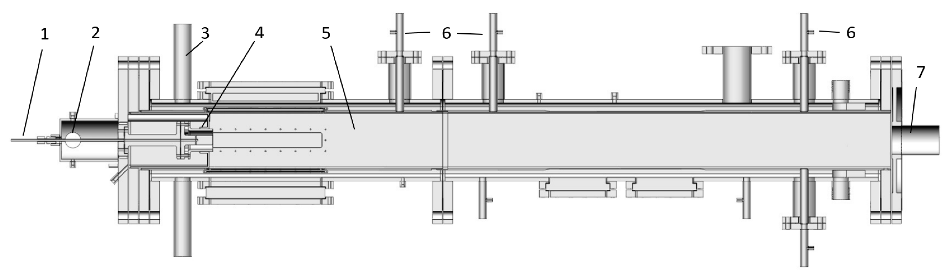
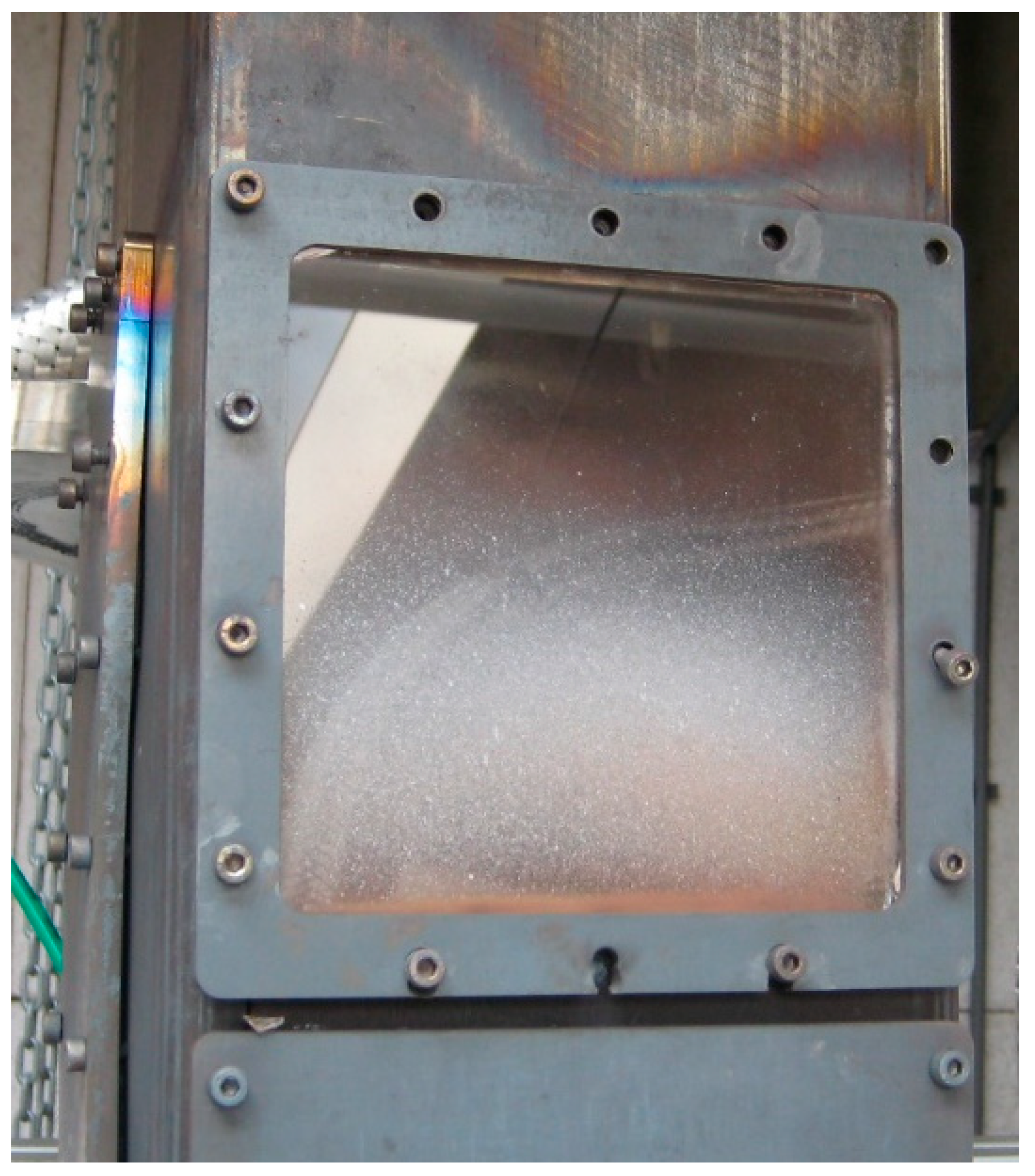
2. Experimental Setup

The experimental investigation was conducted on a swirl stabilized pressurized combustor, as shown in Figure 1. The combustor (called DESIRE) was able to reach 500 kW thermal power at 5 bar absolute pressure, and was operated in premixed mode using natural gas (with 89.12 Mol.% methane and 10.82% nitrogen), and preheated air at 300 °C. A detailed description of the combustor, along with its components and the operational procedure, has been presented in earlier studies [32,33,34]. In this paper, only the relevant components which were essential to the present investigation will be discussed.
The test rig was operated at an air factor of 1.8 and a pressure and thermal power of 1.5 bar/125 kW and 3.0 bar/250 kW, respectively. Air entered the plenum via small holes (12 holes of 10 mm diameter). Due to the high air velocity through these holes and the large area change, the plenum acted as an acoustic decoupler ( R 0.9 ) [34]. The burner was a swirler type with a swirl number of 0.7. It had four fuel injection holes (each 2 mm in diameter) along the circumference of the burner core. The mass flows of air and gas were controlled using Bronckhorst mass flow controller valves, which have an accuracy of 1% of their full scale (500 nm3/h). The injected gas mixed with swirled air in the annular burner channel. The swirler burner opened to the combustion chamber, and thanks to the accompanying formation of the inner and outer recirculation zones in the combustion chamber, the flame was anchored just downstream of the burner. The combustion chamber was a square cross-section rectangular tube with dimensions of 150 × 150 × 1813 mm3 (H × W × L). At the end of the combustor, an exit boundary condition was created by means of a decrease in area ( R 0.7 ) [34]. The purpose of the construction was to reflect acoustic waves back into the combustion chamber, similar to what occurs in a gas turbine engine.
Pressure fluctuations in the combustor were measured using piezoresistive Kulite differential pressure transducers (Kulite XTE 190M) [35]. The Kulite transducer had a 0.35 bar pressure range, and its natural frequency was around 150 kHz. These pressure transducers were able operate at elevated pressures by equalizing the mean pressure on both sides of the sensor diaphragm. The combustor was connected to a pressure supply cylinder, where the amplitude of acoustic oscillations was significantly reduced. Then, this pressure supply cylinder was attached to the back of the pressure transducers using a thin, flexible hose. Due to the volume of the pressure supply cylinder and the viscothermal loss inside the thin hoses, the acoustic energy transmitted from the combustor to the back of the pressure transducers was damped in full to produce a constant background pressure. All the pressure transducers were calibrated with respect to the reference transducer using a calibration tube; thus, relative amplitude and phase errors between the pressure transducers were minimized in order to increase measurement accuracy (see Figure A1).
The experimental data were recorded using a variety of National Instruments DAQ cards. The hardware had three DAQ cards (NI 9239) for input, and one card (NI 9263) for output. These cards were connected to a NI 9188 chassis and linked with a single Ethernet interface back to a host computer. A custom-built LabVIEW script was used to record the data. The script used an averaging algorithm to provide output data. The LabVIEW sampling rate was set to 3125 samples per second, resulting in a total of 10,000 samples being recorded in a duration of 3.2 s. The recorded data were post-processed in the MATLAB 8.0 environment. More details on the experimental procedure are discussed in Appendix A.

Initial Experimental Observations

The experimental investigations were mainly performed at an operating point of 125 kW, 1.5 bar absolute pressure, and an air factor of 1.8. Figure 2 shows the measured pressure spectrum of this operation point. There was distinct activity at 421 Hz and amplitude of 55 Pa. The other activities were below 10 Pa without any distinct peak. This indicates that the spontaneous oscillations were quite well damped due to loss of acoustic energy through the combustor exit and/or a mismatch between the acoustics and combustion dynamics. Due to this, the thermoacoustic feedback was too small to reach limit cycle oscillations, and nonlinear effects and frequency doubling were not observed.
The measured acoustic field was compared with the predicted field using a one-dimensional acoustic network model. Acoustic network models (ANM) are widely used in the prediction of acoustic behavior and combustion instabilities. In the ANM, the whole combustion system is described in a linear approach by a combination of coupled small elements, where the input–output relationship of each element is represented by a transfer matrix. The combination of each transfer matrix in the system is called a system matrix. More details on the system matrix and computational procedure were explained in Appendix A of reference [36]. With the addition of a flame model, the ANM provides the eigenmodes of the system and information on the onset of instabilities. This happens when the determinant of the system matrix (S) is equal to zero. The amplitude of a resulting limit cycle oscillation cannot be predicted, since this is determined by nonlinear high-amplitude behavior.
The system matrix is a function of frequency ω . In the absence of time delays, the determinant of the system is zero for the system’s real eigenfrequencies ω r ; in the presence of time delays, the determinant of the system becomes zero for the system’s complex eigenfrequencies ω r + i ω i . When the complex eigenfrequencies are smaller than zero, the oscillation grows exponentially in time. This indicates the positive growth rate of instabilities. We used the Nelder-Mead simplex search method to find the complex eigenfrequencies [37]. This method employs a direct search approach, eliminating the need for numerical or analytic gradients, and relies solely on function evaluations.
In an earlier study, the one-dimensional acoustic network model was used for a stability analysis on the present experimental test rig [36,38]. The instability analysis results generated in [36,38] are presented in Figure 3. The measured flame transfer function needs to be coupled with the network model, and it is represented there by two analytical models. The first is the well-known n τ σ model, where n represents the interaction index, τ is the certain time delay, and σ is the time delay variance [39]. The second model is the rational transfer function (RTF), as described by Hoeijmakers [40]. It uses a polynomial function to make a fit to the measured flame transfer functions. Figure 3 shows the instability predictions for different FTF implementations. In the first n τ σ model, fit n is kept as constant over the frequency range. In the second n τ σ model, the fit has low pass filter behavior, where the magnitude reduces with increasing frequency. The third fit is according to RTF, and follows the measured FTF as close as possible. These measured and fitted FTFs are presented in Appendix B. All the suggested methods predicted the eigenmodes of the combustor.
The main objective of the study was to gain insight into the sensitivity of the predicted and measured instabilities to the geometrical changes in the test rig. A second objective was to establish the predictive performance of the ANM as a combustor design tool. To research both aspects, the length of the combustor and the exit impedance were varied.

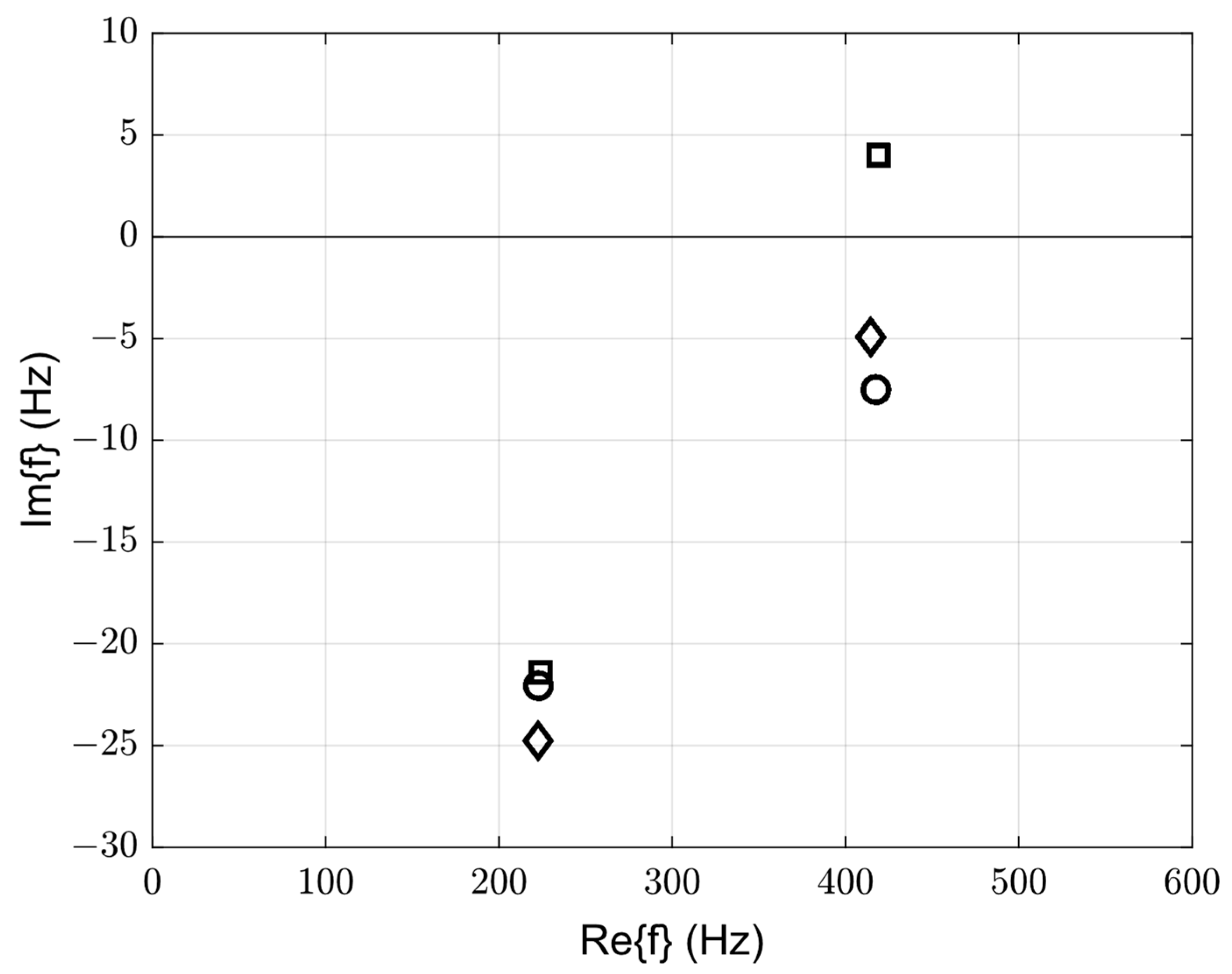
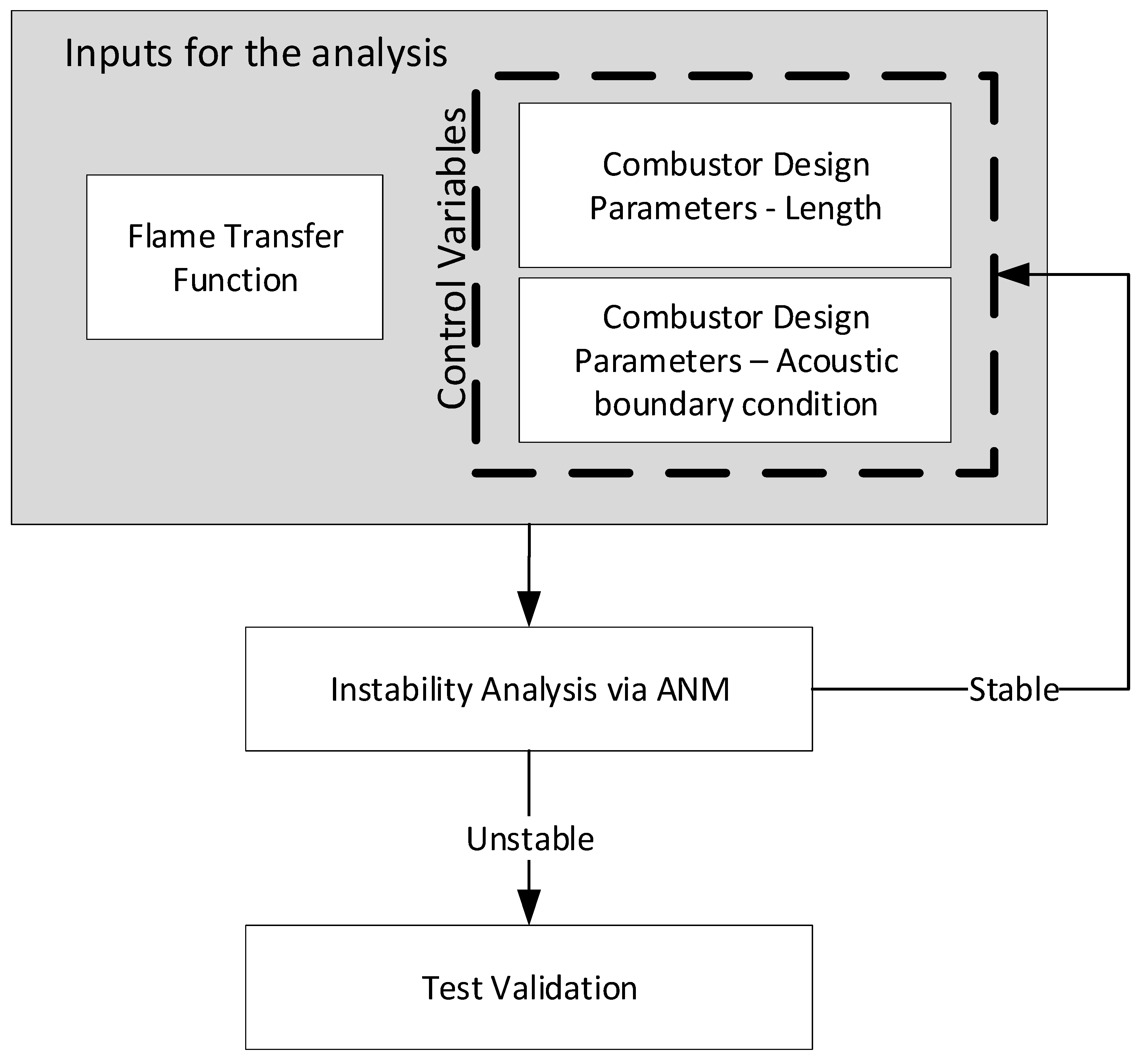
3. Acoustic Design Parameter Change of the Combustion Chamber

This section examines the impact of acoustic design parameters on combustor stability, following the methodology illustrated in Figure 4. The acoustic network model was employed for the purpose of conducting instability analysis. A comprehensive depiction of the network model is provided in Section 3.1. The input parameters are summarized as the flame transfer function, the length of the combustor, and the exit boundary condition of the combustor; they undergo change until the output becomes unstable. The promising configuration is then applied to the experimental setup, and the validation is performed.

3.1. Changing the Length of the Combustion Chamber

The coupling between the heat release rate fluctuation and the combustion chamber acoustics leads to self-excited combustion instabilities. The original design of the UT DESIRE combustor does not exhibit unstable behavior nor high-amplitude combustion oscillations for any operating condition. In this section, the effect of the length of the combustor on thermoacoustic instabilities is investigated, with an aim to reach limit cycle operation. This can be accomplished by coupling an acoustic mode of the combustion chamber to the flame heat release response and by decreasing the loss of acoustic energy at the combustor exhaust.
In the current study, the measured pressure data showed activity only around the second eigenfrequency of the combustor. This suggests that the dynamic of the flame heat release rate was close to, but not matching, the second acoustic eigenfrequency of the combustor. Therefore, the tuning approach was focused on changing the second acoustic eigenfrequency of the combustor to the dynamic response of the heat release rate. The main activity of the heat release rate sits at around 420 Hz. Lee, Gonzalez-Juez, and Figura [10,41,42] experimentally investigated the effect of varying the combustor length in an atmospheric combustor. The length was varied using a plug that could be moved continuously along the length of the combustor (0.76–1.52 m). The results showed that the primary instability mode changed with the combustor length. The strength of the instabilities was weakest for a short combustor length (<0.9 m), and the strongest in the middle length range (0.9–1.2 m).
In the present study, he ANM was further used to determine the optimal length of the combustor and to trigger the unstable mode. The ANM representation of the experimental setup is presented in Figure 5. A hard acoustic boundary was assumed for the air and fuel impedances. A reflection coefficient of 0.7 was applied for the end impedance. The flame transfer function was applied between nodes three and four. In order to take into account a significant liner length and convective outside cooling, the speed of sound (which is dependent on the temperature) varied as a function of the length. The color gradient along the combustion chamber indicated the temperature evolution of the flue gases. The length (L) was varied between 0.9 m and 1.8 m.
Figure 6 shows the instability search for various lengths of the combustor. The ANM model predicted that the first eigenmode of the combustor would shift from 220 Hz to around 420 Hz when the length of the combustor was reduced to 0.9 m. Similarly, the second eigen frequency was also predicted to have moved to a higher frequency range with a decrease in length. The decrease in length showed a change in instability to a smaller growth rate, similar to the findings of [10,41,42]. Apparently, this combination of burner/flame/combustor was in a stable regime, and did not become more unstable with a shorter length. It was interesting to observe that the growth rate increased again for the first eigenfrequency when the length became such that it approached the 420 Hz of the second eigenfrequency at the original length of 1.8 m.

3.2. Changing the Acoustic Boundary Condition

In the DESIRE test rig, a diaphragm is placed at the downstream end of the combustion chamber to provide a well-defined acoustic end-condition. This allows the application of a Neumann end condition in the CFD model of the reactive flow. Paschereit et al. [14] investigated different acoustic boundary settings in the atmospheric combustor, ranging from open- to anechoic-end conditions. The changes resulted in the activation of different instability modes. The reflection of acoustic waves in a contraction or nozzle was explained by Marble and Candel [43] using a linear analysis. The dimensions of the nozzle were assumed to be smaller than the shortest wavelength of the perturbations in the flow. Stow et al. [44] expanded this approach to capture the boundary conditions when circumferential modes were present. Furthermore, Duran and Moreau [45] showed that nozzle acoustical behavior has a strong dependency on frequency. Silva et al. [46] used the same approach and introduced specific terms to account for enthalpy jumps induced by the rotor stages of the compressor and turbines. These were then applied in LES simulations as improved boundary conditions.
In order to describe the acoustic behavior of a flow through a diaphragm, a model described in the work of Durrieu et al. [47] was used. This model was validated by measurements and shown to be able to accurately predict the acoustic behavior of a diaphragm. Here, the flow was considered to be incompressible, which is a valid assumption when the Mach number of the bulk flow is much smaller than one. In the DESIRE test rig configuration, typical velocities are in the range of 100 m/s, while the speed of sound is around 800 m/s, leading to a Mach number of 0.12. The following equations describe the flow through the diaphragm, where S is cross sectional area, p is pressure, u is velocity, and ρ 0 is density (see Figure 7 for the definition of the variables):
S 1 u 1 = S v u v = S 2 u 2 ,
p 1 + ρ 0 2   u 1 2 = p v + ρ 0 2   u v 2 ,
p v S 2 + ρ 0 u v 2 S v = p 2 S 2 + ρ 0   u 2 2 S 2   ,
Equation (1) is the mass balance equation. Equation (2) is the Bernoulli equation, determining the velocity and the pressure in the diaphragm. Downstream of the diaphragm, the flow detaches (sharp edge). The free jet that arises acts as momentum on the stagnant flow downstream of the diaphragm. Equation (3) is the momentum equation with which the pressure and velocity in the flow downstream of the diaphragm can be calculated. As can be seen from Figure 7, the area S v   is not equal to the cross-sectional area of the diaphragm ( S d ) due to the so-called vena-contracta effect.
The contraction factor is defined as Υ = S v / S d . A theoretical contraction factor of π π   +   2 0.6 is often used for an incompressible flow through a slit shaped orifice [47]. This is a result of a calculation by Kirchhoff for an incompressible steady-state 2D flow through a diaphragm in an infinite baffle [48]. Several corrections can be applied to this contraction factor, but these corrections are usually small. Therefore, the Kirchhoff correction factor was used here. The pressure and velocity in the diaphragm, p v and u v , respectively, can be eliminated from Equations (1)–(3). The following equations remain:
p 1 = p 2 + ρ 0 u v 2 2 S 2 S v 1 2 S 2 S 1 1 ,
u 1 = u 2 S 2 S 1 ,
These equations can be linearized with respect to the mean flow properties. Using the solution of the Helmholtz equation, the linearized equations can be written in terms of acoustic pressure amplitudes p + and p , i.e., the amplitude of the pressure wave traveling in the positive x-direction and in the negative x-direction, respectively.
p 1 + + p 1 = p 2 + + p 2 + M 2 S 2 S v 1 2 S 2 S 1 1 p 2 + + p 2 ,
p 1 + + p 1 = p 2 + + p 2 S 2 S 1 ,
in which M 2 is the Mach number at location 2, i.e., u 2 / c 2 , with c 2 the local speed of sound. Equations (6) and (7) describe the relationship between the pressure waves upstream and downstream of the diaphragm and can be used in a one-dimensional acoustic model.
Figure 8 shows the value of the reflection coefficient as a function of the contraction diameter, i.e., 38 mm and 75 mm, and frequency (up to 600 Hz). Calculations were made using the network model for the operating condition of 125 kW at 1.5 pressure. From the figure, it can be seen that the smaller contraction provided a higher reflection coefficient and phase values, indicating termination of a closed end.
In order to assess the effect of the reflection coefficient on the instability of the combustor, an instability analysis was performed. The instability searches for the different contractions are compared in Figure 9. The combustor configuration with a small reflection coefficient showed stable combustion dynamics around 420 Hz, while the system with the high reflection coefficient became more unstable. The latter can be explained by the reduced loss of acoustic energy by the system. Since the value of the contraction did not change the phase behavior of the reflection coefficient (see Figure 8 (bottom)), the eigenfrequencies were not changed.
Figure 10 presents the results of both (i) the variation of the length of the combustor and (ii) the end contraction diameter. It can be observed that in all cases, a decrease in length lead to a more stable operation.
In earlier investigations, the prediction of combustion noise has been studied numerically [36]. This study’s emphasis was on the 75 mm contraction, and the results were in good agreement with the measurements. Thus, a numerical analysis was carried out to investigate the instability for different end contractions. Using the same method but only changing the end contraction of the combustor would provide a good comparison. The computational domain of the combustor is shown in Figure 11. In order to reduce the computational cost, only the ¼ section of the combustor was modeled with symmetry boundary conditions. All relevant sections that might have an influence on the thermoacoustic behavior of the combustor were included in the fluid domain. The experimental work and numerical analysis utilized the same operating point (125 kW at 1.5 bar). A mass flow boundary condition was used for the fuel and air inlets, with an amount of 3.06 g/s of natural gas and 72.47 g/s of air (preheated air at 300 °C). All the walls were assumed to be non-slip and adiabatic, except for the liner wall. In the experimental setup, the liner wall was cooled by a flow of cooling air. This behavior needed to also be taken into account in the simulation; thus, additional simulations were performed to obtain this data [49]. As an exit boundary condition, an average pressure outlet condition was implemented.
The mesh for the computational domain was generated with Ansys Mesh. It contained approximately 1.35 and 1.2 million elements for the 75 mm and 38 mm contraction, respectively. The majority of the elements were located at the swirler, fuel injection, and upstream of the combustion chamber. The mesh of the computational domain is presented in Appendix C. The mesh independence study confirmed that the results were not sensitive to the mesh size [36].
Ansys CFX was used as the simulation tool. This simulation tool has previously been used by several researchers to predict combustion instabilities and flame dynamics [49,50,51,52,53]. The burning velocity model (BVM) was used as a combustion model. The SST turbulence model was applied for the steady-state calculations, whereas the SST-SAS model was used for transient calculations. Detailed discussions on the combustion and turbulent models have been provided in a previous study [36].
Two numerical simulations were performed with two different end contractions. The numerical results of the calculations are shown in Figure 12. All simulation results showed combustion dynamics activity at the 400 Hz range. However, the application of 38 mm contraction did not result in the predicted higher pressure fluctuation amplitude. It was uncertain as to whether the weakly compressible solver of CFX would capture the interaction of acoustic wave propagation and flow acceleration in the combustor exit nozzle in the numerical simulation. It did capture the pressure fluctuations induced by combustion rate fluctuations and the induced velocity fluctuations. The former is an issue which cannot be resolved by switching to compressible solver. According to Keshtiban et al. [54], for low Mach number simulations, compressible flow solvers suffer severe deficiencies, both in accuracy and efficiency.
To sum up, the research that has been conducted so far regarding the ANM has shown that changing the length of the combustor will not cause it to reach limit cycle oscillations. With a decrease in length, the first eigenmode of the combustor shifts towards a higher frequency, but the instability moves towards more stable conditions. On the other hand, tuning the end contraction by reducing its diameter, as indicated by the ANM, results in a shift towards the instability mode. However, CFD simulations did not support the latter finding. Therefore, this change was explored using the available experimental setup. The following section provides detailed experimental observations on the implementation of this change in the setup.

3.3. Experimental Implementation and Observation

As discussed earlier, the stable regime of the combustor with a contraction size of 75 mm was characterized by a relatively low-amplitude combustion noise. This noise was constant in time and could be explained by the balance between the flame dynamics, low reflection of the combustor acoustics, and acoustic wave damping. It was expected that changing the contraction size to 38 mm would result in a stronger coupling between flame dynamics and acoustics. Figure 13 shows both contractions.
Figure 14 compares the experimental observations for the 75 mm contraction and the 38 mm contraction at 125 kW power and an air factor of 1.8. The 75 mm contraction pressure time trace in Figure 14a appears chaotic and irregular. The signal’s amplitude was in the order of hundreds of Pascals, with time-varying amplitudes increasing and decreasing. However, when the 38 mm contraction was introduced, the combustor transitioned into a different combustion regime (Figure 14b), characterized by persistent high-amplitude pressure oscillations that were constant in time. The combustion noise from the stable regime transformed into a humming noise with amplitudes of up to 3000 Pascal. Once this regime was fully developed, the amplitude of the oscillations remained constant over time. For better visibility, a zoomed-in figure is shown for both cases. The time signal for the 75 mm contraction (Figure 14c) showed a very noisy signal, while the 38 mm contraction (Figure 14d) showed an almost perfect sinusoidal wave profile. The red dashed line represents a sinusoidal wave at 426 Hz, fit to the measured time signal.
The plot in Figure 15 shows the signal’s power spectral density as a function of frequency for the 38 mm contraction. The periodic dynamics of the signal in the time domain appear as a narrow and tall peak at 426 Hz. Another notable feature of the spectrum is the presence of peaks due to non-linear phenomena. These peaks occur at frequencies of 856 and 1278 Hz, which are double and triple the instability frequency. This frequency doubling is characteristic of nonlinear behavior at high oscillation amplitudes.
Figure 16 compares the pressure spectrum of the 75 mm contraction to the 38 mm contraction. Both cases showed activity around 420 Hz, while the amplitude of the stable situation was almost 20 times less than the limit cycle oscillation of the 38 mm contraction.
Next to the research on the 1.5 bar and 125 kW thermal power conditions, the investigations were also conducted on 3.0 bar and 250 kW power. Unfortunately, due to the failure of the window, part of the acoustic wave was dissipated, significantly affecting the amplitude of the instabilities. Data from this experiment are presented in Appendix D.

4. Conclusions

The design of a gas turbine combustion chamber using a given burner design and envelope of operation conditions is an important challenge with regard to thermoacoustic stability. In this paper, we investigated the effect of altering the acoustic field boundary conditions on the growth of thermoacoustic oscillations, either by means of a shorter combustion chamber or by employing different reflection coefficients at the exit of the combustion chamber. This was performed for a pressurized laboratory combustor equipped with a premixed natural gas burner using a combination of computational fluid dynamics simulations and a 1D acoustic model, followed by experimental validation. These changes were explored on the available DESIRE test rig. The original design combination of the swirl-stabilizing burner and high-pressure combustor, which operate in a stable regime, was adapted to determine the point at which limit cycle oscillations occurred. The effects of the change in length and of the reflection coefficients on the instability of the combustor-flame combination was investigated using the 1D acoustic network model and flame response data on the basis of the CFD simulation. The changes were chosen such that the flame characteristic parameters were not affected.
Decreasing the combustor length from 1.8 m to 0.9 m resulted in an increase in combustor eigen frequency and a more stable operation (prediction by ANM) compared to the original length of 1.8 m. The ANM-predicted effect of a change in length was found to compare qualitatively well with empirical findings in the literature.
To determine the effect of the exit flow reflection coefficient, experiments were performed on the University of Twente DESIRE test rig. The predictive performance of the ANM as a combustor design tool was demonstrated here, as ANM successfully predicted the system shift towards instability with increased reflection coefficients. This was investigated at 1.5 bar/125 kW operational conditions, and for two dimensions of the contraction tube, i.e., 75 mm and 38 mm outlet dimeter. The system exhibited limit cycle oscillations with a frequency of 426 Hz and SPL amplitude of 150 dB with the small 38 mm exhaust area, whereas for the 75 mm contraction, no significant oscillations were recorded. This validation indicates that the model can be used for combustor design parameter optimization to avoid instability and tune to stable operating regimes of the combustor at the design stage.
In parallel with the ANM based modeling, ANSYS CFX based modeling was employed for the combination of burner and combustor. This was performed using URANS numerical simulations in the combustor system for the conditions as used in the ANM approach to predict the pressure field induced by the rate of combustion fluctuations. While the eigen modes of the combustor were well captured, the CFX numerical computations did not predict an increase in pressure oscillation amplitude at 420 Hz due to the change in reflection coefficient, and the simulation did not reach the limit cycle as observed in the experiments.
These findings demonstrate the need for a systematic approach to designing optimal combinations of pressurized gas turbine engine burners and combustors. These systems exhibit a highly non-linear sensitivity to the geometrical features of the combustion chamber. While the ANM method was demonstrated to give accurate predictions regarding both eigen frequencies and acoustic amplitude as a function of the design parameters, this applied for full CFD simulation only to the eigen frequencies. The CFD-based method failed to predict the effect of a design change on the induced pressure oscillation amplitude. Further research on CFD methods suitable for low Mach number turbulent combustion flows with thermoacoustic effects is required. Carefully conducted experiments supported by acoustic network model predictions are an essential step in understanding thermoacoustic sensitivities and providing adequate thermoacoustic oscillation mitigation solutions.

Author Contributions

Validation, M.K.; Investigation, M.K.; Writing—original draft, M.K.; Supervision, J.B.W.K.; Writing—review and editing, A.K.P.; Writing—review and editing. All authors have read and agreed to the published version of the manuscript.

Funding

This research was funded by EC in the Marie Curie Actions-Networks for Initial training, Project LIMOUSINE with project number [214905].

Data Availability Statement

The original data presented in the study are openly available at https://doi.org/10.4121/b1fcf201-c229-4dd1-a62e-5e07f9b18441.

Conflicts of Interest

The authors declare no conflicts of interest.

Appendix A. Experimental Procedure

The experimental procedure begins with equipment preparation, ensuring the smooth operation of key components such as mass flow controllers and heater controllers, as well as the reliable performance of compressors for gas and air supply. Once the air compressor (screw type driven by a Diesel engine) is primed and ready to deliver air at a pressure of 10 bar, we initiate the flow of air and set the preheater temperature to 300 °C. We await the preheated air to reach a consistent temperature of 280 °C, at which point the ignition process commences by initiating a 35-kW power input at a stoichiometric air-fuel factor (λ) of 1. When flame detection is confirmed, we gradually adjust the air factor, incrementally moving it towards 1.6 over a span of 15 min. During this time, we monitor all equipment, ensuring that thermocouples, pressure sensors, mass flow controllers, and other vital components are delivering stable and reliable readings. When we have confirmed the stability of all equipment and conditions, we proceed to set the desired thermal power output. In the event of an elevated pressure measurement, we take prompt action to adjust the system pressure to match the designated set point. Data collection begins once the designated set point is reached.
In order to minimize the relative amplitude and phase errors between the pressure transducer signals, all the pressure transducers connected to their dedicated amplifier channels are calibrated with respect to the reference transducer and its amplifier channel. To this end, the pressure transducers are mounted at the end flange of a tube, with a loudspeaker mounted at the other end flange. Figure A1 shows the calibration results: amplitude and phase angle of transducer signals 2 and 3 relative to the reference signal of transducer 1. P.T. 1 is the reference pressure transducer, and P.T. 2 and P.T. 3 represent the relative deviation compared to P.T. 1. It can be observed that there is a minor deviation in both amplitude and phase angle as a function of frequency between all transducer signals, hence the calibration.
Figure A1. Calibration of pressure transducers.
Energies 17 01885 g0a1

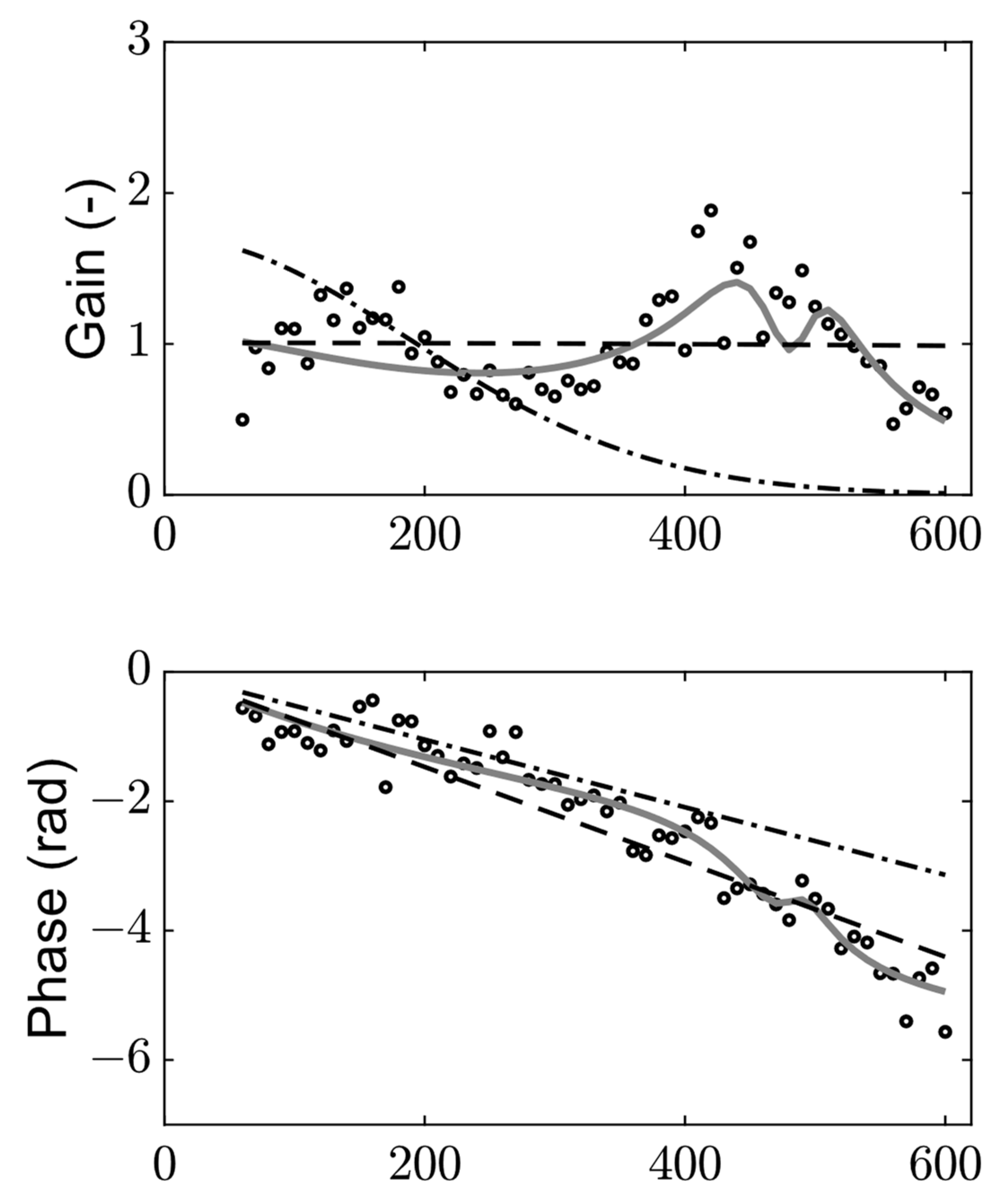
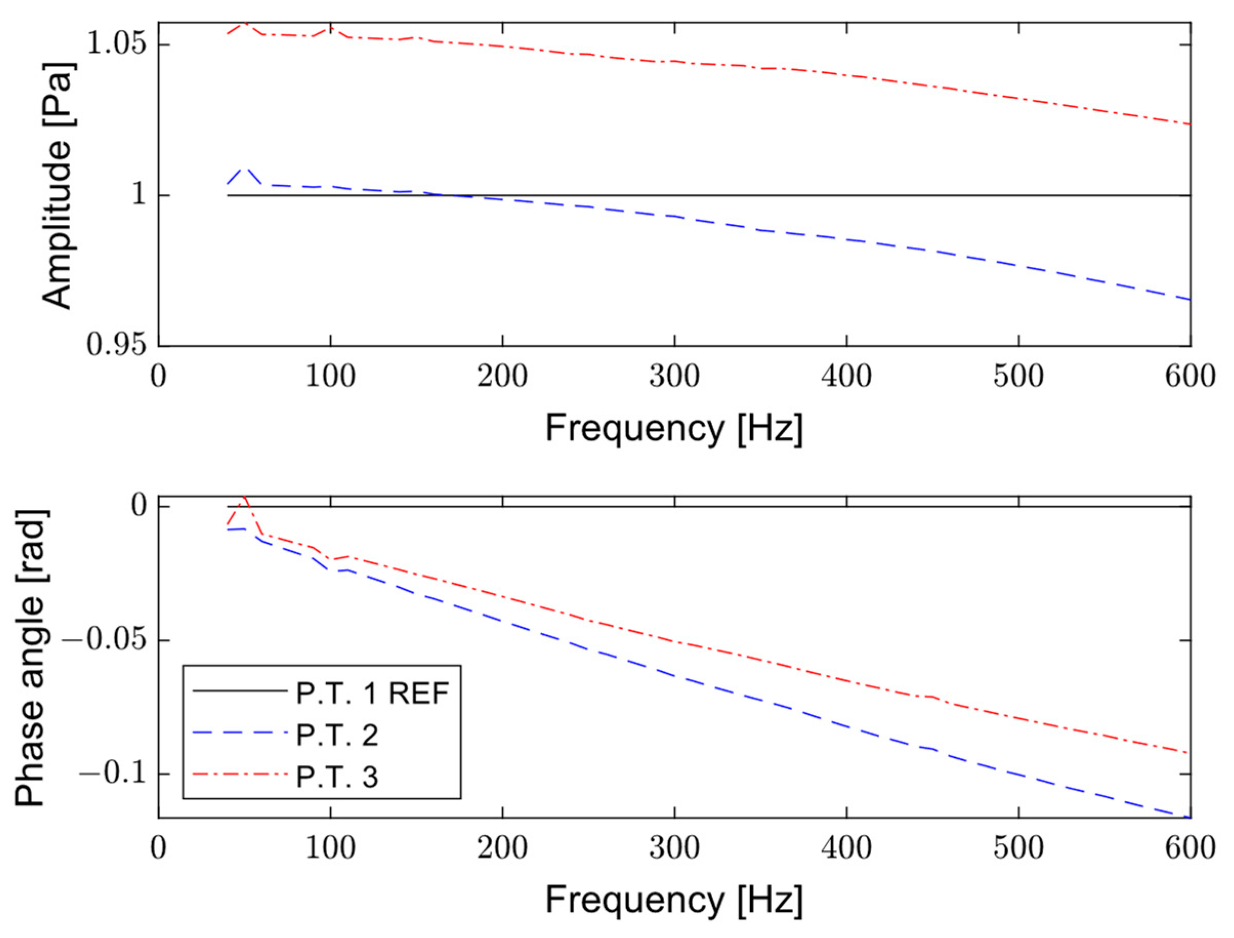
Appendix B. Measured FTF and Parameters for the FTF Fit Models

In this section, the measured FTF and fit parameters for the FTF are presented. The measurement method and the details regarding fits have been explained in detail in a previous work [36,38]. Figure A2 shows the measured and fitted FTFs at the 1.5 bar/125 kW power operation point (15.7). The parameters and the equations used in making the plot are presented in Table A1 for a rational transfer function fit, and Table A2 for n τ σ model fits.
Figure A2. The frequency response of the flame models. Measurement (o), n τ σ model (--), n τ σ model (-.), rational transfer function method (gray -), (PN = 5, PD = 6).
Energies 17 01885 g0a2
H F = ω 5 a 1 ω 4 a 2 ω 3 a 3 ω 2 a 4 + ω a 5 + a 6 ω 6 b 1 + ω 5 b 2 + ω 4 b 3 ω 3 b 4 ω 2 b 5 + ω b 6 + b 7 ,
Table A1. Parameters of the Rational Transfer Function Model FTF fit.
a 1 254.23   i b 1 1
a 2 1084551.95 b 2 6431,017548392937897006049752   i
a 3 1046987085.12   i b 3 28143683,5938770174980163574
a 4 33488605017316,56 b 4 114061616334.2061920166   i
a 5 352954545271784   i b 5 214974463797900.625
a 6 406601584529901289472 b 6 492411166094701952   i
b 7 382766879396415733760
H F = n e i ω t e 1 2 ω 2 σ 2 ,
Table A2. Parameters of nτσ Model FTF fit.
n τ σ
Full fit 1.0072 1.1686   m s 0.0521   m s
Low pass filter 1.705 0.83244   m s 0.84474   m s

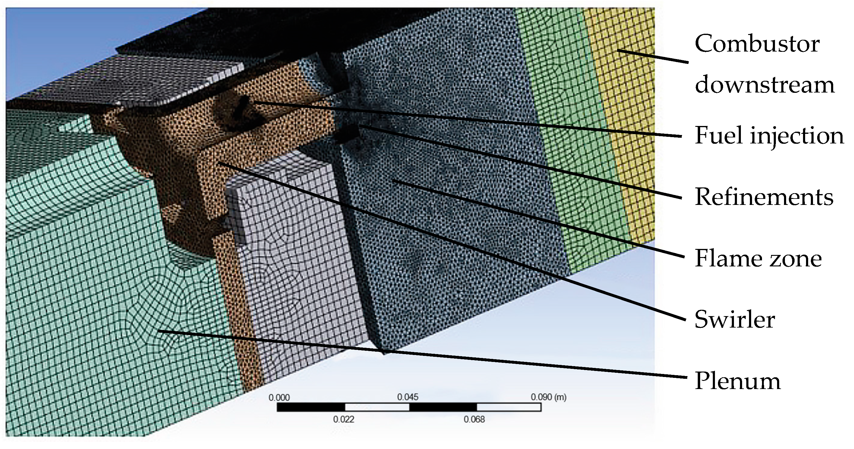
Appendix C. Mesh of the Computational Domain

The Ansys Mesh is used to generate the mesh of the computational domain. The mesh of the most important part of the computational domain is presented in Figure A3. In the earlier investigation the structured and unstructured mesh types were investigated [36]. That study showed that the best configuration would be to use them in combination. Thus, the total element number is kept minimal. The unstructured type of mesh element has a better mesh adaptivity and fits better in complex geometries while the structured type of mesh offers easy data access. Therefore, the fluid domain is divided into sub-sections where different mesh types can be applied. Unstructured tetrahedral meshing is used for the locations for the swirler, annular channel and flame zone in the combustion chamber. These locations have large gradients and high levels of turbulence. Since the flow field is smooth in the plenum and the down-stream section of the combustion chamber a structured type of mesh element can be used there. Detailed mesh statistics for both cases are presented in Table A3.
Figure A3. Mesh of a computational domain.
Energies 17 01885 g0a3
Table A3. Mesh statistics for 38 mm and 75 mm contraction cases.
Contraction diameter38 mm75 mm
Total Number of elements1,194,4701,357,395
Total Number of Tetrahedrons1,057,6821,202,131
Total Number of Prisms51013052
Total Number of Hexahedrons108,588123,538
Total Number of Pyramids23,09928,674

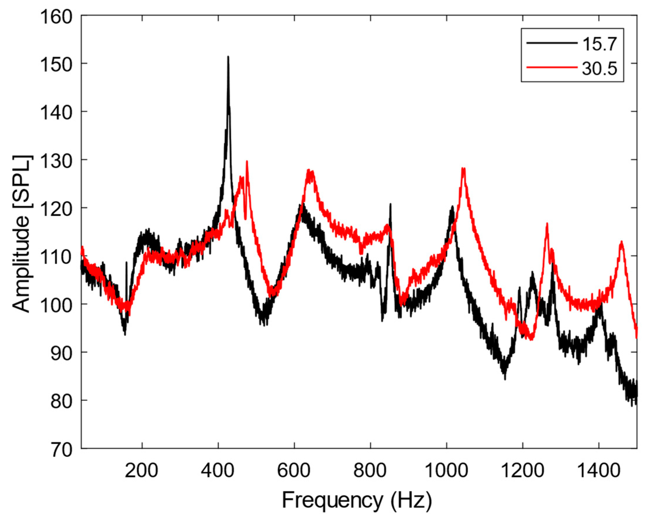
Appendix D. Combustion Test at 3.0 Bar and 250 kW Thermal Power

After having conducted the experiments at 1.5 bar/125 kW, with about one hour limit-cycle operation, the experiments were continued with tests at 3.0 bar and 250 kW at the 38 mm contraction. The measured pressure amplitude SPL spectrum as a function of frequency is presented in Figure A4 for both the 1.5 bar/125 kW and the 3.0/250 kW measurements. The expectation was to find similar spectra with slightly higher (3–6 dB) amplitudes at 250 kW. In Figure A4 it can be observed, however, that the 3.0 bar/250 kW does not have high-amplitude limit cycle oscillations. There is a high peak at slightly over 426 Hz, but the SPL is “only” 130 dB instead of 155 dB as in the 1.5 bar/125 kW case. In order to explore the reason for this, the combustor was partly disassembled and inspected. The liner near the burner features windows that provide an opportunity for visual access to the flame. In these window frames, there are quartz glass windows mounted and fixated by metal flanges using M4 bolts. After disassembly of the combustor liner, it was discovered that of the 14 bolts near the flame area, 7 had failed and gone missing; see Figure A5. This indicates the effect on the combustor assembly and the likelihood of structural failure due to such high-amplitude oscillations. This failure leads to severe acoustic leakage from the inside of the liner to the outside and a large loss of acoustic energy that will prevent amplitude growth, leading to limit cycle oscillation. The bolts most probably failed at the finalization and cooling down of the 1.5 bar/125 kW test. The failing liner window frame after the high-pressure 3 bar test is shown in Figure A5. In view of safety, it was decided to discontinue the test series and not to perform further tests at 3 bar. The target of the research was reached at the 1.5 bar/125 kW test, where it was demonstrated that a contraction to 38 mm could lead to limit cycle oscillations thanks to a decreased loss of acoustic energy from the combustor system. This demonstrates the susceptibility of a gas turbine engine combustor to thermoacoustic instability due to the high acoustic reflection coefficient at the turbine nozzle.
Figure A4. Pressure spectrum for 125 kW at 1.5 bar (15.7) and 250 kW at 3 bar (30.5) as a function of frequency.
Energies 17 01885 g0a4
Figure A5. Failed and missing bolts of the liner window frame of the combustor after the 1.5 bar/125 kW test.
Energies 17 01885 g0a5

References

  1. Lieuwen, T.; Torres, H.; Johnson, C.; Zinn, B.T. A Mechanism of combustion instability in lean premixed gas turbine combustors. J. Eng. Gas Turb. Power Trans. ASME 2001, 123, 182–189. [Google Scholar] [CrossRef]
  2. Campa, G. Prediction of the Thermoacoustic Combustion Instability in Gas Turbines. Ph.D. Thesis, Politecnico di Bari, Bari, Italy, 2012. [Google Scholar]
  3. Candel, S. Combustion dynamics and control: Progress and challenges. Proc. Combust. Inst. 2002, 29, 1–28. [Google Scholar] [CrossRef]
  4. Poinsot, T. Prediction and control of combustion instabilities in real engines. Proc. Combust. Inst. 2017, 36, 1–28. [Google Scholar] [CrossRef]
  5. Syred, N.; Beér, J. Combustion in swirling flows: A review. Combust. Flame 1974, 23, 143–201. [Google Scholar] [CrossRef]
  6. Rayleigh, L. The Theory of Sound; Macmillan and Co.: London, UK, 1896; Volume 2. [Google Scholar]
  7. Poinsot, T.J.; Trouve, A.C.; Veynante, D.P.; Candel, S.M.; Esposito, E.J. Vortex-driven acoustically coupled combustion instabilities. J. Fluid Mech. 1987, 177, 265–292. [Google Scholar] [CrossRef]
  8. Heckl, M.A. Active control of the noise from a rijke tube. J. Sound Vib. 1988, 124, 117–133. [Google Scholar] [CrossRef]
  9. Chen, L.S.; Bomberg, S.; Polifke, W. Propagation and generation of acoustic and entropy waves across a moving flame front. Combust. Flame 2016, 166, 170–180. [Google Scholar] [CrossRef]
  10. Lee, H.J. Combustion Instability Mechanisms in a Lean Premixed Gas Turbine Combustor. Ph.D. Thesis, The Pennsylvania State University, State College, PA, USA, 2009. [Google Scholar]
  11. Kim, D.; Park, S.W. Forced and self-excited oscillations in a natural gas fired lean premixed combustor. Fuel Process. Technol. 2010, 91, 1670–1677. [Google Scholar] [CrossRef]
  12. Evesque, S.; Dowling, A. Adaptive control of combustion oscillations. In Proceedings of the 4th AIAA/CEAS Aeroacoustics Conference, Toulouse, France, 2–4 June 1998. [Google Scholar]
  13. Zhang, J.; Ratner, A. Experimental study of the effects of hydrogen addition on the thermoacoustic instability in a variable-length combustor. Int. J. Hydrog. Energy 2021, 46, 16086–16100. [Google Scholar] [CrossRef]
  14. Paschereit, C.O.; Gutmark, E.; Weisenstein, W. Excitation of thermoacoustic instabilities by interaction of acoustics and unstable swirling flow. AIAA J. 2000, 38, 1025–1034. [Google Scholar] [CrossRef]
  15. Yang, Y.; Wang, G.; Fang, Y.; Jin, T.; Li, J. Experimental study of the effect of outlet boundary on combustion instabilities in premixed swirling flames. Phys. Fluids 2021, 33, 027106. [Google Scholar] [CrossRef]
  16. Sahay, A.; Kushwaha, A.; Pawar, S.A.; PR, M.; Dhadphale, J.M.; Sujith, R.I. Mitigation of limit cycle oscillations in a turbulent thermoacoustic system via delayed acoustic self-feedback. Chaos: Interdiscip. J. Nonlinear Sci. 2023, 33, 043118. [Google Scholar] [CrossRef] [PubMed]
  17. Merk, H. An analysis of unstable combustion of premixed gases. Symp. Int. Combust. 1957, 6, 500–512. [Google Scholar] [CrossRef]
  18. Dowling, A. The calculation of thermoacoustic oscillations. J. Sound Vib. 1995, 180, 557–581. [Google Scholar] [CrossRef]
  19. Schuermans, B.B.H.; Polifke, W.; Paschereit, C.O.; van der Linden, J.H. Prediction of Acoustic Pressure Spectra in Combustion Systems Using Swirl Stabilized Gas Turbine Burners. In ASME Turbo Expo 2000: Power for Land, Sea, and Air; American Society of Mechanical Engineers: New York, NY, USA, 2000. [Google Scholar]
  20. Gentemann, A.; Fischer, A.; Evesque, S.; Polifke, W. Acoustic Transfer Matrix Reconstruction and Analysis for Ducts with Sudden Change of Area. In Proceedings of the 9th AIAA/CEAS Aeroacoustics Conference and Exhibit, Hilton Head, SC, USA, 12–14 May 2003. [Google Scholar]
  21. Kopitz, J.; Polifke, W. CFD-based application of the Nyquist criterion to thermo-acoustic instabilities. J. Comput. Phys. 2008, 227, 6754–6778. [Google Scholar] [CrossRef]
  22. Polifke, W. System modelling and stability analysis. Lect. Ser. Von Karman Inst. Fluid Dyn. 2007, 9, 7. [Google Scholar]
  23. Hubbard, S.; Dowling, A.P. Acoustic Resonances of an Industrial Gas Turbine Combustion System. J. Eng. Gas Turbines Power 2000, 123, 766–773. [Google Scholar] [CrossRef]
  24. Polifke, W.; Poncet, A.; Paschereit, C.; Döbbeling, K. Reconstruction of acoustic transfer matrices by instationary computational fluid dynamics. J. Sound Vib. 2001, 245, 483–510. [Google Scholar] [CrossRef]
  25. Hobson, D.E.; Fackrell, J.E.; Hewitt, G. Combustion instabilities in industrial gas turbines—Measurements on operating plant and thermoacoustic modeling. J. Eng. Gas Turbines Power 2000, 122, 420–428. [Google Scholar] [CrossRef]
  26. Van der Eerden, F. Noise Reduction with Coupled Prismatic Tubes. Ph.D. Thesis, University of Twente, Enschede, The Netherlands, 2000. [Google Scholar]
  27. Martin, C.E.; Benoit, L.; Sommerer, Y.; Nicoud, F.; Poinsot, T. Large-eddy simulation and acoustic analysis of a swirled staged turbulent combustor. AIAA J. 2006, 44, 741–750. [Google Scholar] [CrossRef]
  28. Laera, D.; Campa, G.; Camporeale, S.M.; Bertolotto, E.; Rizzo, S.; Bonzani, F.; Ferrante, A.; Saponaro, A. Modelling of Thermoacoustic Combustion Instabilities Phenomena: Application to an Experimental Test Rig. Energy Procedia 2014, 45, 1392–1401. [Google Scholar] [CrossRef]
  29. Krediet, H.J. Prediction of Limit Cycle Pressure Oscillations in Gas Turbine Combustion Systems Using the Flame Describing Function; University of Twente: Enschede, The Netherlands, 2012. [Google Scholar]
  30. Hantschk, C.-C.; Vortmeyer, D. Numerical simulation of self-excited thermoacoustic instabilities in a rijke Tube. J. Sound Vib. 1999, 227, 511–522. [Google Scholar] [CrossRef]
  31. Gövert, S.; Mira, D.; Kok, J.; Vázquez, M.; Houzeaux, G. Turbulent combustion modelling of a confined premixed jet flame including heat loss effects using tabulated chemistry. Appl. Energy 2015, 156, 804–815. [Google Scholar] [CrossRef]
  32. Kapucu, M.; Kok, J.B.; Alemela, P. Comparison of Two Methods for Flame Transfer Function Measurements: MOOG Valve or Siren and the Impact of Results on the Instability Analysis in a High Pressure Combustor. In Turbo Expo: Power for Land, Sea, and Air; American Society of Mechanical Engineers: New York, NY, USA, 2012. [Google Scholar]
  33. Pozarlik, A. Vibro-Acoustical Instabilities Induced by Combustion Dynamics in Gas Turbine Combustors. Ph.D. Thesis, University of Twente, Enschede, The Netherlands, 2010. [Google Scholar]
  34. Van Kampen, J.F. Acoustic Pressure Oscillations Induced by Confined Premixed Natural Gas Flames. Ph.D. Thesis, University of Twente, Enschede, The Netherlands, 2006. [Google Scholar]
  35. Kulite Netherlands, Stekon B.V. Meer Duin 64b, 2163 HC Lisse, The Netherlands. Available online: https://kulite.com//assets/media/2022/09/XTE-190-1.pdf (accessed on 26 March 2024).
  36. Kapucu, M.; Kok, J.B.W. CFD-Based Prediction of Combustion Dynamics and Nonlinear Flame Transfer Functions for a Swirl-Stabilized High-Pressure Combustor. Energies 2023, 16, 2515. [Google Scholar] [CrossRef]
  37. Lagarias, J.C.; Reeds, J.A.; Wright, M.H.; Wright, P.E. Convergence Properties of the Nelder-Mead Simplex Method in Low Dimensions. SIAM J. Optim. 1998, 9, 112–147. [Google Scholar] [CrossRef]
  38. Kapucu, M.; Kok, J.B.W.; Pozarlik, A. Experimental investigation of thermoacoustics and high frequency combustion dynamics with band stop characteristics in a pressurized combustor. Energies 2024, 7, 1680. [Google Scholar] [CrossRef]
  39. Schuermans, B. Modeling and Control of Thermoacoustic Instabilities. Ph.D. Thesis, Ecole Polytechnique Federale De Lausanne, Lausanne, Switzerland, 2003. [Google Scholar]
  40. Hoeijmakers, P.M. Flame-Acoustic Coupling in Combustion Instabilities. Ph.D. Thesis, Technische Universiteit Eindhoven, Eindhoven, The Netherlands, 2014. [Google Scholar]
  41. Gonzalez, E.; Lee, J.; Santavicca, D. A study of combustion instabilities driven by flame-vortex interactions. In Proceedings of the 41st AIAA/ASME/SAE/ASEE Joint Propulsion Conference & Exhibit, Tucson, AZ, USA, 11–13 July 2005. [Google Scholar]
  42. Figura, L.; Lee, J.G.; Quay, B.D.; Santavicca, D.A. The effects of fuel composition on flame structure and combustion dynamics in a lean premixed combustor. In ASME Turbo Expo 2007: Power for Land, Sea, and Air; American Society of Mechanical Engineers: New York, NY, USA, 2007. [Google Scholar]
  43. Marble, F.; Candel, S. Acoustic disturbance from gas non-uniformities convected through a nozzle. J. Sound Vib. 1977, 55, 225–243. [Google Scholar] [CrossRef]
  44. Stow, S.R.; Dowling, A.P.; Hynes, T.P. Reflection of circumferential modes in a choked nozzle. J. Fluid Mech. 2002, 467, 215–239. [Google Scholar] [CrossRef]
  45. Duran, I.; Moreau, S. Solution of the quasi-one-dimensional linearized Euler equations using flow invariants and the Magnus expansion. J. Fluid Mech. 2013, 723, 190–231. [Google Scholar] [CrossRef]
  46. Silva, C.F.; Durán, I.; Nicoud, F.; Moreau, S. Boundary conditions for the computation of thermoacoustic modes in combustion chambers. AIAA J. 2014, 52, 1180–1193. [Google Scholar] [CrossRef]
  47. Durrieu, P.; Hofmans, G.; Ajello, G.; Boot, R.; Aurégan, Y.; Hirschberg, A.; Peters, M.C.A.M. Quasisteady aero-acoustic response of orifices. J. Acoust. Soc. Am. 2001, 110, 1859–1872. [Google Scholar] [CrossRef] [PubMed]
  48. Pierce, A.D. Acoustics: An Introduction to Its Physical Principles and Applications; Acoustic Society of America: New York, NY, USA, 1994. [Google Scholar]
  49. Ozcan, E. Tuning the self-excited thermo-acoustic oscillations of a gas turbine combustor to Limit Cycle Operations by means of numerical analysis. Master’s Thesis, University of Twente, Enschede, The Netherlands, 2012. [Google Scholar]
  50. Shahi, M.; Kok, J.B.W.; Pozarlik, A.K.; Casado, J.C.R.; Sponfeldner, T. Sensitivity of the Numerical Prediction of Turbulent Combustion Dynamics in the Limousine Combustor. J. Eng. Gas Turbines Power 2014, 136, 021504. [Google Scholar] [CrossRef]
  51. Shahi, M. Modeling of Complex Physics & Combustion Dynamics in a Combustor with a Partially Premixed Turbulent Flame. Ph.D. Thesis, University of Twente, Enschede, The Netherlands, 2014. [Google Scholar]
  52. van Kampen, J.F.; Kok, J.B.W.; van der Meer, T.H. Efficient retrieval of the thermo-acoustic flame transfer function from a linearized CFD simulation of a turbulent flame. Int. J. Numer. Methods Fluids 2007, 54, 1131–1149. [Google Scholar] [CrossRef]
  53. Louis, J.J.; Kok, J.B.; Klein, S.A. Modeling and measurements of a 16-kW turbulent nonadiabatic syngas diffusion flame in a cooled cylindrical combustion chamber. Combust. Flame 2001, 125, 1012–1031. [Google Scholar] [CrossRef]
  54. Keshtiban, I.; Belblidia, F.; Webster, M. Compressible flow solvers for low Mach number flows—A review. Int. J. Numer. Methods Fluids 2004, 23, 77–103. [Google Scholar]
Figure 1. DESIRE experimental setup. (1) Fuel inlet, (2) Air inlet, (3) Cooling air inlet, (4) Swirler burner, (5) Combustion chamber, (6) Pressure sensor locations, (7) Exhaust.
Energies 17 01885 g001
Figure 2. Pressure spectra of the combustor (measured acoustic oscillation amplitude as a function of frequency).
Energies 17 01885 g002
Figure 3. Instability analysis. n τ σ model (◊), n τ σ model (low pass filter) (□), RTF (○).
Energies 17 01885 g003
Figure 4. Flowchart for the methodology.
Energies 17 01885 g004
Figure 5. 1D acoustic network model representation of the experimental setup.
Energies 17 01885 g005
Figure 6. Instability analysis for different length of the combustor. Light gray color represents the length of the combustor equal to 0.9 m, and black color represents the length of 1.8 m.
Energies 17 01885 g006
Figure 7. Flow through a diaphragm [47].
Energies 17 01885 g007
Figure 8. Reflection coefficient calculations depending on the contraction diameter. Reflection coefficient magnitude (top) and phase (bottom) vs. frequency.
Energies 17 01885 g008
Figure 9. Instability searches for different contraction diameter.
Energies 17 01885 g009
Figure 10. Instability searches for different contraction diameter and length of the combustor. (■) represents the 38 mm contraction; (●) represents 75 mm.
Energies 17 01885 g010
Figure 11. Computation domain. (1) Air inlet, (2) Plenum, (3) Swirler, (4) Fuel inlet, (5) Combustion chamber, (6) Exhaust (end contraction).
Energies 17 01885 g011
Figure 12. Pressure spectrum for different contraction diameters (acoustic pressure amplitude as a function of frequency for two end conditions).
Energies 17 01885 g012
Figure 13. End contraction: (a) 75 mm, seen from the downstream side, (b) 38 mm, seen from the upstream side.
Energies 17 01885 g013
Figure 14. Quality of measured time signal. (a) 75 mm contraction, (b) 38 mm contraction, (c) zoomed in time signal for 75 mm contraction, (d) zoomed in signal for 38 mm contraction with sinusoidal fit (red dashed line).
Energies 17 01885 g014aEnergies 17 01885 g014b
Figure 15. Measured pressure spectrum amplitude in sound pressure level (SPL) (dB ref. pressure 20 μPa) as a function of frequency.
Energies 17 01885 g015
Figure 16. Pressure spectrum for contraction diameters 75 and 38 mm.
Energies 17 01885 g016
Disclaimer/Publisher’s Note: The statements, opinions and data contained in all publications are solely those of the individual author(s) and contributor(s) and not of MDPI and/or the editor(s). MDPI and/or the editor(s) disclaim responsibility for any injury to people or property resulting from any ideas, methods, instructions or products referred to in the content.

