Abstract
Electric arc furnace technology is a key factor in the sustainable transformation of the iron and steel industry. This study compares two discrete-time multi-objective optimization models—integer and mixed-integer linear programming—that integrate unit commitment with economic and environmental dispatch. After evaluating both approaches, the integer linear programming model is used, due to its reasonable calculation time, to assess demand-side management potentials under real-world processes and day-ahead market conditions. The model is applied to various scenarios with differing energy price dynamics, CO2 pricing, EAF utilization levels, and weighting of the objective functions. Results indicate cost savings of up to 6.95% and CO2 emission reductions of up to 10.86%, though these are subject to a non-linear trade-off between economic and environmental goals. Due to process constraints and market structures, EAFs’ flexibility in energy carrier use (switch between electricity and natural gas) is limited to 3.07%. Additionally, lower furnace utilization does not necessarily increase flexibility, as downstream process requirements restrict scheduling options. The study underscores the importance of green electrification, with up to 36% CO2 savings when using 100% renewable electricity. Overall, unlocking industrial flexibility requires technical solutions, supportive market incentives, and regulatory frameworks for effective industrial decarbonization.
1. Introduction
Addressing global climate change and advancing energy transition toward a low-carbon society requires accelerating industrial measures [1]. Alongside new technologies, grid expansion, restructuring energy markets, and renewable integration, demand-side management (DSM) is key to bridging the gap between increasingly volatile energy generation and inflexible demand. DSM includes a broad portfolio of measures to be able to utilize different flexibility potentials, rather than offering a singular solution [2], and can be classified into energy efficiency (EE) and demand response (DR) measures [3]. DR has recently gained attention as a cost-effective way to enhance demand-side flexibility (DSF) [4]. Options include load shifting, where consumption is rescheduled without changing total demand [5], load shedding, where consumption is temporarily decreased, without later compensation [6], and energy carrier flexibility (ECF), i.e., switching temporarily between energy sources to lower demand peaks while keeping processes running [7].
The potential and effectiveness of DSM measures differ significantly across sectors. Residential loads provide limited and highly dispersed flexibility [8], electric vehicles (EVs) face high operational costs, slow response, and battery degradation [9], and commercial buildings struggle with complex management, reliability, and short lifespans [10]. Industry, by contrast, accounts for about one-third of global energy consumption [11], and, especially, energy-intensive industry sectors are interesting in terms of DR [12]. Yet, industrial production is highly complex, with interdependent processes and strict operational constraints. Many studies analyze industry in a generalized way, combined with a high-level perspective, neglecting site- and process-specific constraints [12,13]. Such approaches estimate theoretical potentials but do not identify realizable ones. More detailed studies focus mainly on load shifting or shedding and economic process logistics, while overlooking emissions or systemic effects [14,15,16,17,18,19,20,21]. ECF, in particular, remains underexplored in industrial applications.
1.1. Iron and Steel Industry and the EAF Process
The iron and steel sector is, alongside cement, the most energy- and emission-intensive industry worldwide, accounting for 7% of greenhouse gas emissions in 2021 [22]. Traditionally dominated by the blast furnace—basic oxygen furnace (BF-BOF) route, the industry has increasingly shifted toward electric arc furnaces (EAFs). Scrap-based EAF production emits only 0.3–0.6 t CO2 per ton of crude steel, compared to the 1.6–2.2 t CO2 of the BF-BOF route [22,23,24,25], making it a key technology for efficiency improvements and decarbonization [26,27]. Owing to the adaptability to different feedstocks (scrap, direct reduced iron (DRI), sponge iron) and the ability to integrate both electrical and chemical energy carriers, EAFs are expected to further expand their share in global production [22,28].
In the EAF, scrap is batch-wise melted into liquid steel (one batch of liquid metal is called “a heat”). Although seemingly straightforward, EAF operation is highly complex due to its non-linear, time-varying load, extreme conditions, limited measurement possibilities, multiphysical interactions, and strong parameter interdependencies, which leads to the fact that the fundamental understanding of EAF operation is still not perfect. Decision-making during operation, due to low levels of automation, still depends on the operator’s involvement to a vast extent [29,30]. Therefore, EAFs have been the subject of extensive research, ranging from detailed heat and mass transfer models [31,32,33] and data-driven energy consumption models [34,35,36,37,38,39,40,41] to studies of arc energy transfer [42,43,44] and high-level scheduling approaches [15,29,45,46,47,48,49,50,51,52,53,54,55].
EAFs are among the most significant loads on power grids [56,57], affecting both external networks [2,58,59] and internal plant equipment and processes [60,61]. Their specific energy consumption ranges from 510 to 880 kWh/t of crude steel, depending on scrap composition and steel quality [28]. Alternative current EAFs typically use three graphite electrodes in combination with natural gas burners. A heat comprises several phases: energy-extensive preparation, charging and energy-intensive melting (usually of three scrap baskets), fining (for chemical adjustment), and tapping into a refractory-lined ladle. Figure 1 illustrates the time-resolved electricity and gas demand as well as the heat-wise ratio (proportion of electricity to natural gas) of a typical EAF operation. More information about the investigated EAF can be found in a previous publication [62].
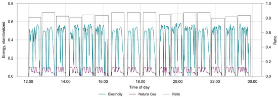
Figure 1.
Electricity and gas demand (primary y-axis) and ratio (secondary y-axis) of an EAF.
Efficient energy use is critical for industrial competitiveness, as energy can represent up to 20% of production costs [2,29]. Integrated scheduling and control tools can improve EAF efficiency and unlock operational flexibility [30]. In addition to these economic aspects, growing and interdependent environmental concerns further increase the need for smarter energy use [63].
1.2. Integer Linear and Mixed-Integer Linear Multi-Objective Optimization Problems in Industry
Unit Commitment (UC) problems, common in power system operation, determine the schedule of generation units to meet demand at minimal cost while respecting operational constraints such as ramping limits or start-up costs [64,65,66]. With the increasing share of renewables, UC has become more complex due to higher uncertainty and variability [67]. Another central task is Economic Dispatch (ED), which minimizes generation costs and, in its extended form as Economic and Environmental Dispatch (EED), explicitly incorporates environmental objectives [68,69,70]. EED highlights the inherent trade-off between cost efficiency and ecological impact, making it a constrained, multi-objective optimization (MOO) problem [30]. While dispatch and DSM were long viewed as separate, and even complementary, topics, recent research emphasizes their complementarity [71].
Optimization problems can be classified by mathematical structure. Integer Linear Programming (ILP) relies on linear relations with integer values, whereas Mixed-Integer Linear Programming (MILP) also includes continuous variables, allowing more versatile real-world applications [72]. The drawback of MILP is its higher computational effort, often requiring advanced solvers such as CPLEX or Gurobi. In contrast to deterministic optimization formulations, (meta-)heuristics, like artificial intelligence or relaxation techniques, are suitable especially for larger, more complex problems [73].
MOO addresses situations with multiple, often conflicted, objectives. Instead of a single optimum, a set of Pareto-optimal solutions is generated, reflecting the trade-offs among criteria. None of these solutions dominates the others; rather, they provide decision-makers with alternatives aligned to specific priorities. Common methods to approximate the Pareto front include the weighting method, ε-constraint method, and goal programming [69,74,75]. A general mathematical formulation of a minimization MOO problem is [76]:
where is the vector of decision variables defining the decision space X, y the vector of objectives, and and the constraints.
In EED problems, reducing emissions typically increases operational costs or alters scheduling. MOO thus provides a systemic framework to explore these trade-offs, enabling decision-makers to balance economic and environmental priorities rather than relying on a single objective.
1.3. State of Research
Recent energy and power system optimization research increasingly focuses on optimal control strategies and dispatch models beyond traditional ED and UC, as flexibilization of industrial processes is key to reducing costs, responding to volatile electricity prices, and supporting renewable integration. The topic of EED has been extensively studied, including integrated regional multi-energy systems with carbon trading schemes and polluting control technologies [77], as well as combined heat and power units and storage [78,79]. Renewables are considered through static and dynamic ED [80], uncertainties of photovoltaic (PV) and wind power [81], and misestimation of wind power [82]. From a market perspective, a spatially and temporally resolved dispatch model was built [83], which simulates the electricity market and physical constraints of various components in the electricity grid. Methods range from MILP or MINLP to machine learning algorithms, such as genetic algorithms and meta-heuristics.
Industrial applications have traditionally focused on ED, but environmental aspects are gaining importance. Optimization for load dispatch in industrial environments must consider site-specific complexities [84,85] and the potential impact of changes on overall efficiency [86]. For instance, an MILP-based energy management framework for a tire manufacturer incorporates EVs, RES, and demand response [85], while the magnesium industry applies optimal dispatch strategies integrating RES and process constraints to reduce costs [84]. In the cement industry, coordination frameworks based on model predictive control (MPC) regulate mills in combination with storage [4]. Generic, integer load models for batch processes reduce peak demand and electricity costs [15], and real-time optimization of submerged arc furnaces (SAFs) enhances grid stability, lowers operational costs, and integrates RES [87]. ECF has also been studied using optimal control theory, while maintaining sulfur emission limits [88].
Several works address the energy-intensive iron and steel industry. Examples include applying a non-dominated sorting genetic algorithm (NSGA) to optimize environmentally relevant technologies in China [89], or a continuous-time MILP approach for steel plant scheduling under energy constraints [51]. Market mechanisms such as day-ahead pricing, time-of-use tariffs, peak pricing, or critical peak pricing significantly affect DR in steel production. Extending scheduling horizons can improve performance but increases complexity [13]. One study models steel plant consumption against a pre-specified demand curve, penalizing deviations. The MILP model with a continuous-time formulation, applied to two EAFs, demonstrates that production costs can be reduced [53]. A MINLP model optimizes surplus byproduct gas to reduce the operating costs of the steam power system [90], while ladle furnaces are studied as flexibility providers with real-time evaluation indices [91].
Regarding EAFs, a coordinated dispatch framework models smelting and low-power states, adjusting production cycles to minimize costs while meeting productivity goals [92]. A shrinking-horizon non-linear MPC approach with a detailed dynamic model addresses multivariable interactions and time-varying prices, maximizing profit opportunities [18]. Other works develop mathematical EAF models to minimize energy consumption, and one proposes a linear time-invariant model and linear programming formulation to minimize costs based on electricity and electrode consumption [29]. Load stabilization through time-sharing across multiple EAFs has been studied with a hybrid genetic algorithm—particle swarm optimization (GA-PSO) [60]. From a broader perspective, EAF scheduling has been integrated into dual timescale frameworks for coordinated wind power utilization, combining day-ahead DR with intra-day battery and thermal scheduling, reducing curtailment and emissions [93]. Coordinated strategies between wind and industrial loads show potential for grid stability but introduce trade-offs in labor and maintenance [12]. Further DSM methods for EAFs combine ampacity techniques to raise net power output without new infrastructure [2], while trade-offs between electrode wear and operating intensity under varying electricity prices highlight the complex interplay of consumption, heating, and equipment lifespan [57].
1.4. Research Needs
As the largest electricity consumer in an electric steel plant and one of the largest on the power grid, EAFs are expected to play a central role in industrial DSM. They are frequently described as highly flexible due to rapid start-up/shutdown behavior and the ability to quickly adjust their operation modes [57,93,94]. A deeper understanding of the internal mechanics may uncover untapped flexibility potential [13], but also challenge existing assumptions when production demands, market dynamics, or cost structures shift. The current literature addresses various EAF topics, yet detailed bottom-up flexibilization strategies beyond aggregate load shifting remain scarce. Few studies consider the impact of operating times on downstream logistics and productivity. Moreover, many assume idealized system conditions (e.g., full-state measurement), thereby estimating theoretical potentials not transferable to practice. An underexplored option is ECF, relevant for EAFs operated with both electrcity and natural gas, directly affecting costs and CO2 emissions. Similar to UC in power systems, industrial processes could adapt their energy demand and mix based on price volatility and emission factors, contributing to cost savings and decarbonization. Expanding EED methodologies from power systems to industrial processes could therefore enhance DSF and support a more sustainable energy system.
This study investigates the potential of a combined UC and EED MOO for an EAF to evaluate realizable potentials for cost and emission reduction via ECF, narrowing the gap between theoretical and realizable flexibility. It examines framework conditions under different energy market scenarios, critically reassessing the assumption of a fully flexible EAF. The optimization model is formulated as both a MILP and an ILP optimization problem in Python 3.9, using the gurobipy library (version 12.0.3) and the Gurobi solver (version 12.0.0). The optimizer shifts heat start times and, unlike traditional load shifting, dynamically adjusts the electricity-to-gas ratio depending on market conditions. Because higher electricity shares prolong heat duration, temporal load shifting is essential, which, as far as the authors know, has not been addressed previously. Constraints ensure fulfillment of process requirements such as productivity, logistics, and technical limits. The objective function minimizes energy costs—including electricity, natural gas, CO2 costs under the European Union Emissions Trading System, grid charges, and taxes from 2024—while also reducing direct and indirect CO2 emissions. The analysis further considers market fluctuations, the transition toward green electricity, and EAF utilization.
This work addresses the following research questions:
Q1: Which methodological approach is best suited to the EAF optimization problem in the context of DSF in terms of accuracy, robustness, and calculation time?
Q2: How do cost and emission benefits evolve under different process and market scenarios?
Q3: How much ECF can be realized, quantified by the amount of energy shifted between energy carriers?
The paper is structured as follows: Section 2 describes materials and methods, including data, the optimization model(s), and parameters of the sensitivity analysis. Section 3 presents results and discussion, and Section 4 concludes with key findings and an outlook for further research in this area.
2. Materials and Methods
2.1. Data and Preparation
The study uses historic production and energy market data from 2024 to demonstrate the value of optimizing EAF operation with ECF under realistic process conditions. Operating data from “Stahl- und Walzwerk Marienhütte GmbH” (Graz, Austria) included time-resolved load profiles and process-relevant information for each heat. For confidentiality, all data were normalized, preserving methodological validity and transferability to similar EAF operations.
Day-ahead electricity prices from the European Energy Exchange (EEX) for the Austrian bidding zone were applied (EUR/MWh, 15-min resolution, from 2024) [95]. Fixed cost components (grid fees, taxes on Entso-e grid level 3) were added to reflect total costs. Day-ahead gas prices from the Central European Gas Hub (CEGH) were used as daily values (EUR/MWh) [96], likewise including fixed components. CO2 certificate prices (EUR/t) were obtained from Energy Exchange Austria (EXAA) [97], and the time-varying CO2 footprint of the electricity mix was derived from Nowtricity [98].
Following the design of the European day-ahead market, the optimization horizon spans 36 h, as auctions provide binding prices from 12:00 on the current day until 23:59 of the next.
For data preparation, heat phase durations (preparation, melting, fining, tapping) were rounded to the nearest minute. Atypical heats, defined over heat durations deviating more than ±25% from the mean, were excluded and replaced by representative heats reflecting typical process sequences. Gas consumption, originally measured as volume flow (m3/h), was converted using a lower heating value of 9.97 kWh/m3 [99], enabling direct comparability with electricity consumption.
2.2. Optimization Model
Two optimization models, an ILP and a MILP model, were developed to map the EAF scheduling and enable method comparison. The following discusses modeling assumptions, constraints, objective functions, solver, and key differences.
2.2.1. General Modeling and Assumptions
A central factor is the dependence of heat duration on the energy ratio r between electricity and natural gas, defined as:
where Eel is electrical and Echem is chemical energy input (natural gas) per heat. From production data, the lower bound for r is 85%. Increasing r lengthens the heat duration; a fully electric heat is about 30% longer than one at r = 0.85, though technically feasible. The extension of the heat duration is related to the change in the flow dynamics in the furnace vessel and the heat transfer between the energy source and the scrap or melt. The literature confirms that chemical energy can reduce heat duration under certain conditions [28].
This relationship is modeled linearly:
with:
where theat,original is the baseline duration and r0 the reference ratio.
Total energy per heat remains constant, and changing r only redistributes energy over time. A higher electrical share stretches the load profile, lowering demand without altering total consumption [28].
Time is discretized into one-minute steps to balance fidelity and efficiency. Given typical heat durations and the 36 h optimization horizon, this resolution adequately represents process dynamics while aligning with real-world scheduling practices and available data.
2.2.2. Constraints
To represent operational boundaries and process requirements, the following constraints are incorporated:
- Heat continuity: Once started, a heat must run uninterrupted. Each heat can therefore only be scheduled once:with the binary decision variable zi,r,s ∈ {0,1}, indicating whether heat i starts at time s with ratio r. This three-index structure captures all feasible combinations of heats, ratios, and start times.
- Start time variable: To simplify further constraints, the explicit start time ti of a heat is defined as:
This avoids repeatedly summing over all indices when defining order or pause constraints.
- Fixed sequence: The order of heats is fixed, as their exact duration and energy consumption are only known after completion. Allowing reordering would create unrealistic conditions and distort results.
- Breaks between heats: Operational logistics require short pauses between heats:with di as duration of heat i, a minimum pause of 1 min, and a maximum pause of 20 min, reflecting process logistics (ladle furnace buffering, continuous casting).
2.2.3. Objective Function
The objective function minimizes total energy costs and CO2 emissions of all scheduled heats via a weighted multi-objective approach.
For each heat i, ratio r, and potential start time s, the energy costs Ci,r,s are precomputed as:
and CO2 emissions as:
and denote the electricity and natural gas consumption of a heat i at time step t, and the respective energy prices, and the fixed costs, and the CO2 price applied to the gas-related emissions. and are the specific CO2 emission factors for electricity and gas.
Values are normalzied to [0, 1] for comparability. The final objective combines both with weight α:
where α = 1 corresponds to pure economic dispatch, and α = 0 to ecological dispatch.
The model is solved with Gurobi [100], a state-of-the-art solver known for speed, robustness, and industrial applicability.
2.2.4. Differences Between the ILP and MILP Models
The ILP model uses only binary and integer variables, whereas the MILP model extends this with continuous ones. The key difference is the treatment of the energy ratio r: in the ILP model: r is discretized (85–100% in 0.5% steps), while in the MILP model, it is continuous. This enables a more precise determination of electricity–gas shares, but at the cost of significantly higher computational effort. A continuous r requires coupling with interpolated heat duration, generation of additional energy profiles, and numerous auxiliary variables to link constraints, ensuring, e.g., that time-resolved energy quantities are only active when a heat is running.
These dependencies are modeled with Big-M constraints, a standard technique and mathematical switch to linearize logical conditions (“if-then”) by introducing a large constant M, effectively switching variables on or off via binary indicators. In the MILP model, they ensure conditions such as “set energy to zero if the EAF is off,” e.g.:
with xi,t as the binary start indicator, eel,l(i) the planned electric demand, and zel,l the helper variable linking them. This coupling must be applied for every heat, time step, and local index within a heat, generating millions of variables and inequalities. In contrast, the ILP remains compact, requiring only a binary choice of predefined energy-mix options and one start variable per heat. While its coarser discretization of r causes small accuracy losses in energy mix and heat duration, it enables solutions within reasonable time.
2.3. Scenario Definition, Parameter Variation, and Key Performance Indicators
To test robustness and assess the influence of market, policy, and process conditions, a sensitivity analysis was performed for a Representative day, defined as the average of all sample days. Economic and ecological boundary conditions were systematically varied (Table 1) to evaluate impacts on optimal EAF scheduling and estimate industrial DSM potential. For a fully renewable electricity system (Austria’s 2030 goal), a CO2 intensity of 32.15 g/kWh was assumed [98,101].

Table 1.
Parameters and their variation range for the sensitivity analysis.
Seasonal scenarios (Spring, Summer, Autumn, Winter) were added, based on mean daily values using meteorological boundaries. In addition, two extraordinary days (Extraordinary #1 in May, Extraordinary #2 in September) with unusual market characteristics were analyzed. Table 2 shows the price characteristics of the different scenarios, and Figure 2 illustrates the volatile electricity day-ahead prices.
Table 2.
Price and emitted CO2 equivalent characteristics for the sensitivity analysis scenarios [95,98,101].
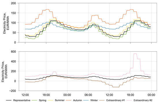
Figure 2.
Day-ahead electricity price curves for sensitivity analysis scenarios [95].
Three key performance indicators (KPIs) evaluate the sensitivity results:
- Cost change (ΔC): percentage difference between optimized and original costs (negative = reduction).
- Emission change (ΔE): defined analogously.
- Energy Carrier Flexibility (ECF): ratio of electricity to total energy input.
3. Results and Discussion
3.1. ILP vs. MILP
Both models were compared regarding structure, complexity, and solution performance to justify the choice of ILP for subsequent analyses. For 50 heats over 36 h, the ILP model comprises ~3.35 million variables and ~200 constraints, mainly from binary variables for start time and energy-mix selection. The MILP, in contrast, introduces continuous performance variables for each time step and corresponding binaries with Big-M couplings, resulting in ~14.8 million variables and ~29 million constraints (Table 3). This difference is reflected in computational effort: with the same optimality gap, the ILP model solved in 12 min, whereas the MILP model required 96 h. The latter’s weak relaxations and vast solution space severely slow convergence.
Table 3.
Differences and results of the (M)ILP models for 50 heats and a 36 h time horizon.
Quantitative results also differ slightly: the MILP model achieved a cost change ΔC of –1.34% and an emission change ΔE of +0.01%, compared to –0.35% and +0.50% for the ILP model. While the MILP model yields marginally better outcomes by allowing continuous ratios r, its computational cost outweighs this benefit. Thus, the ILP model—though restricted to discrete energy-mix ratios—provides near-optimal solutions within practical runtimes. For this study, applicability is decisive; therefore, the ILP model was retained as the working basis.
3.2. Sensitivity Analysis
The Representative scenario shows a cost reduction of 2.83% through optimal EAF scheduling, under given assumptions and process constraints. Figure 3 illustrates cost reductions under ±50% price variations (electricity, gas, CO2 certificates), and Table 4 summarizes the results. The electricity price has the strongest impact: a 50% decrease in electricity prices reduces costs by 1.80%, whereas a 50% increase enhances the cost reduction to 3.45%. The optimizer shifts production to low-price periods or favors gas-driven operation when electricity prices rise. Gas price variation has a smaller but inverse effect, with savings ranging from 3.51% (–50% gas price) to 2.18% (+50%). CO2 certificate prices exert the least influence, with reductions of between 2.67% (+50%) and 2.99% (–50%), reflecting their relatively low cost share.
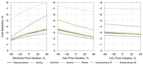
Figure 3.
Price sensitivities for day-ahead electricity, gas, and CO2 certificate prices.
Table 4.
Parameters and results of price sensitivity analysis.
Seasonal scenarios show only marginal differences (Figure 3), possible cost reduction clustering near the Representative value (min. 2.40% in Winter, max. 2.96% in Spring), confirming model robustness under typical market conditions. In contrast, the two extraordinary scenarios yield markedly higher savings: 4.20% (Extraordinary #1) and up to 6.95% (Extraordinary #2). Across all scenarios, price variations follow the same patterns observed for the Representative case.
Overall, the optimization consistently delivers cost savings under standard conditions and scales its benefits with price volatility, demonstrating its value as a flexibility-enabling tool for industrial energy management.
At first glance, lower capacity utilization might suggest greater cost-saving and flexibility potential. However, when process continuity is realistically considered, this correlation no longer holds. Imposing a maximum idle time of 20 min—reflecting continuous casting requirements—restricts the optimizer’s ability to freely allocate downtime. Cost reduction thus depends not only on idle periods but on the interaction between utilization level and feasible scheduling flexibility.
Table 5 shows that for Spring, Summer, and Extraordinary #1, maximum savings occur at 95% EAF utilization, while for Autumn, Winter, and Extraordinary #2, the optimum is at 90% EAF utilization. Below these levels, cost reductions persist but diminish. The results demonstrate a non-linear relationship: moderate utilization (90–95%) best balances technical feasibility and economic benefit.
Table 5.
Cost reduction potentials for EAF utilization grade variation.
3.3. Environmental and Ecological Dispatch
In addition to economic considerations, the impact of the used electricity mix’s CO2 footprint was evaluated. Besides the global plans to increasingly generate electricity from renewable sources, Austria has set the explicit goal of achieving 100% renewable electricity by 2030. While costs remain unaffected (prices are exogenous), emissions decline substantially: across all scenarios, CO2 emissions are reduced by 32% (economic optimization, α = 1) to 36% (ecological optimization, α = 0) on average when fully renewable electricity is assumed (see Table 6). This highlights the critical role of green electrification as a prerequisite for achieving substantial decarbonization in electric steel production. The results also underline the dynamic relationship between the extent of the CO2 footprint of electricity and emission reduction, as in seasons with a low CO2 footprint (e.g., Spring or Summer), the values for emission reduction are smaller than in seasons where the electricity CO2 footprint is high (e.g., Autumn).
Table 6.
Emission reduction for ecological and economic optimization.
Under current conditions, however, economic optimization generally increases emissions. Gas remains price-wise attractive despite CO2 costs, leading the optimizer to favor natural gas. Resulting emission changes range from +9.08% (α = 1) to –4.88% (α = 0). With fully renewable electricity, the span is +9.54% to –5.13%.
The ratio r reflects this trade-off: with α = 0, the average r is 0.89, but higher values are limited by longer heat durations, which restrict productivity. As α rises, r decreases to 0.85 (α = 1). Ecological optimization yields more variable r patterns across the horizon, while economic optimization keeps r low and stable (see Figure A1 in Appendix A).
Additionally, Pareto fronts were generated for all scenarios (Figure 4) and highlight the non-linear cost–emission trade-off. In the Representative scenario, α = 1 reduces costs (–2.83%) but raises emissions (+5.19%); α = 0 lowers emissions (–2.79%) with a small cost increase (+0.74%). Intermediate α values shift smoothly along the curve, showing that marginal gains in emission reduction require disproportionately higher costs, and vice versa (Table 7).
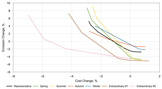
Figure 4.
Pareto fronts for different scenarios.
Table 7.
Parameters and results of EED.
Seasonal differences confirm this: in Spring and Summer, ecological optimization achieves up to −4.88% emissions at modest cost penalties, making them favorable for ecological dispatch. In Autumn and Winter, higher CO2 intensity of electricity limits benefits; Pareto fronts are flatter, with smaller changes (Autumn: −1.41% vs. +2.62%). Extraordinary scenarios deviate: Extraordinary #2 achieves the highest cost reduction (−6.95%), with even moderate α values delivering both cost savings and emission cuts. Extraordinary #1 yields slightly lower savings (−4.20%) but exhibits a steeper front, reflecting stronger conflict between objectives.
Across the seasonal scenarios (Spring, Summer, Autumn, Winter), the shape and location of the Pareto fronts differ: In Spring and Summer, electricity is cheaper and has a relatively low carbon footprint, which increases the ecological optimization potential. This is reflected in higher values for possible emission reduction (−4.68% in Spring, and −4.88% in Summer) for ecological optimization. At the same time, the cost differentials between ecological and economic objectives remain modest, indicating that environmental improvements can be achieved without disproportionately high economic sacrifices. This makes Spring and Summer particularly favorable for ecological dispatch strategies.
The model was also used to evaluate the ECF over the 36 h optimization horizon and quantify the energy amount that can be shifted between electricity and natural gas (relative to the original electricity use). Seasonal scenarios show ECF shifts from +1.65% (α = 0) to −3.07% (α = 1). Extraordinary scenarios exhibit similar ranges (−2.32% to −2.48%). The α-threshold at which electricity becomes favorable differs by scenario: in Autumn, the shift occurs at lower values (α ≈ 0.25) due to high electricity and gas prices with moderate CO2 costs. In Extraordinary #2, high volatility and elevated prices across all carriers drive similar effects (Table 2).
4. Conclusions
This work provides a realistic estimation of EAF flexibility potentials, challenging the common assumption that the full EAF load can be shifted freely. In practice, process constraints—such as thermal balance and process continuity—limit flexibility significantly. The analysis shows that only a fraction of total EAF demand can be reallocated without violating feasibility, and it provides answers to the three research questions defined in Section 1.4:
Q1: Which methodological approach is best suited to the EAF optimization problem in the context of DSF in terms of accuracy, robustness, and calculation time?
The ILP formulation proved well-suited for modeling EAF operation under real-world constraints. Compared to the MILP formulation, it provides robust and transparent results with practical runtimes (3–90 min for a 36 h horizon), which are suitable for use in the real world. For certain combinations of low utilization (<90%) and specific market conditions, computation time may rise, limiting applicability.
Q2: How do cost and emission benefits evolve under different process and market scenarios?
The price sensitivity analysis showed that electricity prices have the strongest impact and are characterized by an inverse relation: higher electricity prices result in greater cost reduction potential, as the optimizer favors using natural gas. Gas and CO2 price effects are weaker but relevant. Seasonal analysis highlights that Spring and Summer—with low prices and CO2 intensity—favor ecological dispatch. Volatile or extreme markets offer the highest savings. This correlates with the finding from the literature [92] that highly regulated electricity prices restrict flexible utilization.
Lower EAF utilization does not necessarily improve flexibility, as the need for a continuous supply of downstream processes restrict the optimizer’s freedom. Advantages are governed by a complex interplay of process constraints and the temporal rearrangement of heats. Therefore, the highest advantages can be achieved at a utilization level between 90% and 95%.
The study confirms the critical importance of green electrification, as a full switch to renewable electricity would reduce emissions by up to 36% across all scenarios. The convex Pareto fronts reveal the non-linear cost–emission trade-off: ecological gains typically entail economic sacrifices, and vice versa.
Q3: How much ECF can be realized, quantified by the amount of energy shifted between energy carriers?
Under current conditions, up to 3.07% of demand can be shifted between carriers. This challenges assumptions of the full-load DSM potential of EAFs. Yet, these realizable load shifts remain substantial and system-relevant, particularly given the growing role of EAFs worldwide. Importantly, these savings entail no additional investment, operational restrictions, or productivity losses.
Results show that the achievable ECF is scenario-dependent and varies with the optimization objective, highlighting that neither full electrification nor complete fuel switching is universally optimal or technically feasible. This underscores the need for targeted incentives and dynamic pricing to steer toward low-carbon pathways.
Overall, technical or process flexibility alone is insufficient for industrial decarbonization. Regulatory signals—dynamic gas and CO2 pricing, grid incentives, and revenues for flexibility—are essential to unlock potential for industrial DSF. Implementing the approach in practice further requires integration of optimization with operating and control systems, though many sites still lack sufficient digitalization.
Assuming the technical feasibility of heat-wise EAF operation, the model provides a valuable decision-support tool for economic and ecological optimization. Current limitations lie in the adjustment of energy-source ratios only on a heat basis; finer phase-level modeling would increase accuracy but also computational demand. While this study focused on the day-ahead market, extensions to intraday optimization, flexibility marketing, or storage integration could further strengthen industrial contributions to energy system flexibility and climate goals. Future research should therefore prioritize advancing digitalization in energy-intensive industries and developing fast, robust optimization methods to enable practical use of flexibility across time horizons and market contexts.
Author Contributions
Conceptualization, V.Z.; Data curation, V.Z.; Formal analysis, V.Z.; Funding acquisition, T.K.; Investigation, V.Z. and A.G.; Methodology, V.Z. and A.G.; Project administration, V.Z.; Resources, V.Z. and T.K.; Software, V.Z. and A.G.; Supervision, T.K.; Validation, V.Z. and A.G.; Visualization, V.Z.; Writing—original draft, V.Z.; Writing—review and editing, V.Z. and T.K. All authors have read and agreed to the published version of the manuscript.
Funding
This work was carried out as part of the DSM_OPT project. DSM_OPT is a subproject of NEFI—New Energy for Industry, an innovation network funded by Climate and Energy Funds Austria.
Data Availability Statement
Restrictions apply to the availability of these data. Data were obtained from Stahl- und Walzwerk Marienhütte GmbH and are available with the permission of Stahl- und Walzwerk Marienhütte GmbH.
Acknowledgments
During the preparation of this manuscript/study, the author(s) used ChatGPT 4.0 and Grammarly (v1.2.146.1631) for grammar checking, paraphrasing, and enhancing readability. The authors have reviewed and edited the output and take full responsibility for the content of this publication.
Conflicts of Interest
The authors declare no conflicts of interest. The funders had no role in the design of the study; in the collection, analyses, or interpretation of data; in the writing of the manuscript; or in the decision to publish the results.
Abbreviations
The following abbreviations are used in this manuscript:
| BF-BOF | Blast furnace and basic oxygen furnace |
| CEGH | Central European Gas Hub |
| DR | Demand response |
| DRI | Direct reduced iron |
| DSF | Demand-side flexibility |
| DSM | Demand-side management |
| EAF | Electric arc furnace |
| ECF | Energy carrier flexibility |
| EE | Energy efficiency |
| EEX | European Energy Exchange |
| EXAA | Energy Exchange Austria |
| EED | Economic and environmental dispatch |
| EV | Electric vehicles |
| GA-PSO | Genetic algorithm-particle swarm optimization |
| ILP | Integer linear programming |
| KPI | Key performance indicator |
| MILP | Mixed-integer linear programming |
| MOO | Multi-objective optimization |
| MPC | Model predictive control |
| NSGA | Non-dominated sorting genetic algorithm |
| PV | Photovoltaic |
| UC | Unit commitment |
Appendix A

Figure A1.
Development of r for different α-values in the Representative scenario.
Figure A1.
Development of r for different α-values in the Representative scenario.

References
- Xu, M.; Lin, B. Leveraging carbon label to achieve low-carbon economy: Evidence from a survey in Chinese first-tier cities. J. Environ. Manag. 2021, 286, 112201. [Google Scholar] [CrossRef]
- Manana, M.; Zobaa, A.F.; Vaccaro, A.; Arroyo, A.; Martinez, R.; Castro, P.; Laso, A.; Bustamante, S. Increase of capacity in electric arc-furnace steel mill factories by means of a demand-side management strategy and ampacity techniques. Int. J. Electr. Power Energy Syst. 2021, 124, 106337. [Google Scholar] [CrossRef]
- Ranaboldo, M.; Aragüés-Peñalba, M.; Arica, E.; Bade, A.; Bullich-Massagué, E.; Burgio, A.; Caccamo, C.; Caprara, A.; Cimmino, D.; Domenech, B.; et al. A comprehensive overview of industrial demand response status in Europe. Renew. Sustain. Energy Rev. 2024, 203, 114797. [Google Scholar] [CrossRef]
- Zhang, X.; Hug, G.; Kolter, J.Z.; Harjunkoski, I. Model predictive control of industrial loads and energy storage for demand response. In Proceedings of the 2016 IEEE Power & Energy Society General Meeting, Boston, MA, USA, 17–21 July 2016. [Google Scholar]
- Fridgen, G.; Häfner, L.; König, C.; Sachs, T. Providing Utility to Utilities: The Value of Information Systems Enabled Flexibility in Electricity Consumption. J. Assoc. Inf. Syst. 2016, 17, 537–563. [Google Scholar] [CrossRef]
- Fridgen, G.; Keller, R.; Thimmel, M.; Wederhake, L. Shifting load through space–The economics of spatial demand side management using distributed data centers. Energy Policy 2017, 109, 400–413. [Google Scholar] [CrossRef]
- Haupt, L.; Körner, M.-F.; Schöpf, M.; Schott, P.; Fridgen, G. Strukturierte Analyse von Nachfrageflexibilität im Stromsystem und Ableitung eines generischen Geschäftsmodells für (stromintensive) Unternehmen. Z. Energiewirtsch. 2020, 44, 141–160. [Google Scholar] [CrossRef]
- Saleh, S.A.; Pijnenburg, P.; Castillo-Guerra, E. Load Aggregation From Generation-Follows-Load to Load-Follows-Generation: Residential Loads. IEEE Trans. Ind. Appl. 2017, 53, 833–842. [Google Scholar] [CrossRef]
- Badji, A.; Abdeslam, D.O.; Chabane, D.; Benamrouche, N. Real-time implementation of improved power frequency approach based energy management of fuel cell electric vehicle considering storage limitations. Energy 2022, 249, 123743. [Google Scholar] [CrossRef]
- Scharnhorst, L.; Sloot, D.; Lehmann, N.; Ardone, A.; Fichtner, W. Barriers to demand response in the commercial and industrial sectors—An empirical investigation. Renew. Sustain. Energy Rev. 2024, 190, 114067. [Google Scholar] [CrossRef]
- Greening, L.A.; Boyd, G.; Roop, J.M. Modeling of industrial energy consumption: An introduction and context. Energy Econ. 2007, 29, 599–608. [Google Scholar] [CrossRef]
- Cai, G.; Zhou, J.; Wang, Y.; Zhang, H.; Sun, A.; Liu, C. Multi-objective coordinative scheduling of system with wind power considering the regulating characteristics of energy-intensive load. Int. J. Electr. Power Energy Syst. 2023, 151, 109143. [Google Scholar] [CrossRef]
- Gholian, A.; Mohsenian-Rad, H.; Hua, Y. Optimal Industrial Load Control in Smart Grid. IEEE Trans. Smart Grid 2016, 7, 2305–2316. [Google Scholar] [CrossRef]
- Arellano, J.; Carrión, M.; García-Cerezo, Á. Optimal Medium-Term Electricity Procurement for Cement Producers. IEEE Access 2024, 12, 54934–54952. [Google Scholar] [CrossRef]
- Ashok, S. Peak-load management in steel plants. Appl. Energy 2006, 83, 413–424. [Google Scholar] [CrossRef]
- Avilés, F.N.; Etchepare, R.M.; Aguayo, M.M.; Valenzuela, M. A mixed-integer programming model for an integrated production planning problem with preventive maintenance in the pulp and paper industry. Eng. Optim. 2023, 55, 1352–1369. [Google Scholar] [CrossRef]
- Castro, P.M.; Westerlund, J.; Forssell, S. Scheduling of a continuous plant with recycling of byproducts: A case study from a tissue paper mill. Comput. Chem. Eng. 2009, 33, 347–358. [Google Scholar] [CrossRef]
- Da Silva, F.A.M.; Moretti, A.C.; Azevedo, A. A Scheduling Problem in the Baking Industry. J. Appl. Math. 2014, 2014, 964120. [Google Scholar] [CrossRef]
- Danket, T.; Tanachutiwat, S.; Rungreunganun, V. Designing advance production planning and scheduling optimization model for reduce total cost of the cement production process under time-of-use electricity prices. In Proceedings of the IEEE 8th International Conference on Industrial Engineering and Applications, Kyoto, Japan, 23–26 April 2021. [Google Scholar]
- Helin, K.; Käki, A.; Zakeri, B.; Lahdelma, R.; Syri, S. Economic potential of industrial demand side management in pulp and paper industry. Energy 2017, 141, 1681–1694. [Google Scholar] [CrossRef]
- Pan, R.; Wang, Q.; Li, Z.; Cao, J.; Zhang, Y. Steelmaking-continuous casting scheduling problem with multi-position refining furnaces under time-of-use tariffs. Ann. Oper. Res. 2022, 310, 119–151. [Google Scholar] [CrossRef]
- International Energy Agency. Iron and Steel Technology Roadmap: Towards More Sustainable Steelmaking; International Energy Agency: Paris, France, 2021. [Google Scholar]
- Toktarova, A.; Karlsson, I.; Rootzén, J.; Göransson, L.; Odenberger, M.; Johnsson, F. Pathways for Low-Carbon Transition of the Steel Industry—A Swedish Case Study. Energy 2020, 13, 3840. [Google Scholar] [CrossRef]
- Arens, M.; Worrell, E.; Eichhammer, W.; Hasanbeigi, A.; Zhang, Q. Pathways to a low-carbon iron and steel industry in the medium-term—The case of Germany. J. Clean. Prod. 2017, 163, 84–98. [Google Scholar] [CrossRef]
- Fan, Z.; Friedmann, S.J. Low-carbon production of iron and steel: Technology options, economic assessment, and policy. Joule 2021, 5, 829–862. [Google Scholar] [CrossRef]
- Tan, X.; Li, H.; Guo, J.; Gu, B.; Zeng, Y. Energy-saving and emission-reduction technology selection and CO2 emission reduction potential of China’s iron and steel industry under energy substitution policy. J. Clean. Prod. 2019, 222, 823–834. [Google Scholar] [CrossRef]
- Sakamoto, Y.; Tonooka, Y.; Yanagisawa, Y. Estimation of energy consumption for each process in the Japanese steel industry: A process analysis. Energy Convers. Manag. 1999, 40, 1129–1140. [Google Scholar] [CrossRef]
- Kirschen, M.; Risonarta, V.; Pfeifer, H. Energy efficiency and the influence of gas burners to the energy related carbon dioxide emissions of electric arc furnaces in steel industry. Energy 2009, 34, 1065–1072. [Google Scholar] [CrossRef]
- Bai, E. Minimizing Energy Cost in Electric Arc Furnace Steel Making by Optimal Control Designs. J. Energy 2014, 2014, 620695. [Google Scholar] [CrossRef][Green Version]
- Shyamal, S.; Swartz, C.L. Real-time energy management for electric arc furnace operation. J. Process Control 2019, 74, 50–62. [Google Scholar] [CrossRef]
- Çamdalı, Ü.; Tunç, M. Modelling of electric energy consumption in the AC electric arc furnace. Int. J. Energy Res. 2002, 26, 935–947. [Google Scholar] [CrossRef]
- Logar, V.; Dovžan, D.; Škrjanc, I. Mathematical Modeling and Experimental Validation of an Electric Arc Furnace. ISIJ Int. 2011, 51, 382–391. [Google Scholar] [CrossRef]
- MacRosty, R.D.M.; Swartz, C.L.E. Dynamic Modeling of an Industrial Electric Arc Furnace. Ind. Eng. Chem. Res. 2005, 44, 8067–8083. [Google Scholar] [CrossRef]
- Andonovski, G.; Tomažič, S. Comparison of data-based models for prediction and optimization of energy consumption in electric arc furnace (EAF). IFAC-PapersOnLine 2022, 55, 373–378. [Google Scholar] [CrossRef]
- Carlsson, L.; Samuelsson, P.; Jönsson, P. Using Interpretable Machine Learning to Predict the Electrical Energy Consumption of an Electric Arc Furnace. In Proceedings of the 4th European Steel Technology and Application Days 2019 (ESTAD 2019), Düsseldorf, Germany, 24–28 July 2019. [Google Scholar]
- Carlsson, L.S.; Samuelsson, P.B.; Jönsson, P.G. Using Statistical Modeling to Predict the Electrical Energy Consumption of an Electric Arc Furnace Producing Stainless Steel. Metals 2020, 10, 36. [Google Scholar] [CrossRef]
- Carlsson, L.S.; Samuelsson, P.B.; Jönsson, P.G. Modeling the Effect of Scrap on the Electrical Energy Consumption of an Electric Arc Furnace. Processes 2020, 8, 1044. [Google Scholar] [CrossRef]
- Chen, C.; Liu, Y.; Kumar, M.; Qin, J. Energy consumption modelling using deep learning technique—A case study of EAF. Procedia CIRP 2018, 72, 1063–1068. [Google Scholar] [CrossRef]
- Dock, J.; Janz, D.; Weiss, J.; Marschnig, A.; Kienberger, T. Time- and component-resolved energy system model of an electric steel mill. Clean. Eng. Technol. 2021, 4, 100223. [Google Scholar] [CrossRef]
- Gajic, D.; Savić-Gajic, I.; Savic, I.; Georgieva, O.S.G. Modelling of electrical energy consumption in an electric arc furnace using artificial neural networks. Energy 2016, 108, 132–139. [Google Scholar] [CrossRef]
- Manojlović, V.; Kamberović, Ž.; Korać, M.; Dotlić, M. Machine learning analysis of electric arc furnace process for the evaluation of energy efficiency parameters. Appl. Energy 2022, 307, 118209. [Google Scholar] [CrossRef]
- Bhonsle, D.C.; Kelkar, R.B. Analyzing power quality issues in electric arc furnace by modeling. Energy 2016, 115, 830–839. [Google Scholar] [CrossRef]
- Chen, F.; Sastry, V.V.; Venkata, S.S.; Athreya, K.B. A Robust Markov-Like Mode for Three Phase Arc Furnaces. In Proceedings of the Caribbean Colloquium on Power Quality, Dorado, Puerto Rico, 24–27 June 2003; Volume 2003. [Google Scholar]
- Moghadasian, M.; Alenasser, E. Modelling and Artificial Intelligence-Based Control of Electrode System for an Electric Arc Furnace. J. Electromagn. Anal. Appl. 2011, 03, 47–55. [Google Scholar] [CrossRef]
- Colla, V.; Matino, I.; Cirilli, F.; Jochler, G.; Kleimt, B.; Rosemann, H.; Unamuno, I.; Tosato, S.; Gussago, F.; Baragiola, S.; et al. Improving energy and resource efficiency of electric steelmaking through simulation tools and process data analyses. Matér. Tech. 2016, 104, 602. [Google Scholar] [CrossRef]
- Li, L.; Li, H. Forecasting and optimal probabilistic scheduling of surplus gas systems in iron and steel industry. J. Cent. South Univ. 2015, 22, 1437–1447. [Google Scholar] [CrossRef]
- Zhao, J.Y.; Wang, Y.J.; Xi, X. Simulation of Steel Production Logistics System Based on Multi-Agents. Int. J. Simul. Model. 2017, 16, 167–175. [Google Scholar] [CrossRef]
- Cao, J.; Pan, R.; Xia, X.; Shao, X.; Wang, X. An efficient scheduling approach for an iron-steel plant equipped with self-generation equipment under time-of-use electricity tariffs. Swarm Evol. Comput. 2021, 60, 100764. [Google Scholar] [CrossRef]
- Cheng, Z.; Zhang, P.; Wang, L. Oxygen Demand Forecasting and Optimal Scheduling of the Oxygen Gas Systems in Iron- and Steel-Making Enterprises. Appl. Sci. 2023, 13, 11618. [Google Scholar] [CrossRef]
- Ferretti, I.; Zanoni, S.; Zavanella, L. Energy Efficiency in a Steel Plant using Optimization-Simulation. In Proceedings of the 20th European Modeling and Simulation Symposium, Amantea, Italy, 17–19 September 2008. [Google Scholar]
- Haït, A.; Artigues, C. On electrical load tracking scheduling for a steel plant. Comput. Chem. Eng. 2011, 35, 3044–3047. [Google Scholar] [CrossRef][Green Version]
- Harjunkoski, I.; Grossmann, I.E. A Decomposition Approach for the Scheduling of a Steel Plant Production. Comput. Chem. Eng. 2001, 2001, 1647–1660. [Google Scholar] [CrossRef]
- Nolde, K.; Morari, M. Electrical load tracking scheduling of a steel plant. Comput. Chem. Eng. 2010, 34, 1899–1903. [Google Scholar] [CrossRef]
- Wang, J.; Wang, Q.; Sun, W. Optimal power system flexibility-based scheduling in iron and steel production: A case of steelmaking–refining–continuous casting process. J. Clean. Prod. 2023, 414, 137619. [Google Scholar] [CrossRef]
- Zhang, X.; Hug, G.; Harjunkoski, I. Cost-Effective Scheduling of Steel Plants with Flexible EAFs. IEEE Trans. Smart Grid 2017, 8, 239–249. [Google Scholar] [CrossRef]
- Marulanda-Durango, J.J.; Zuluaga-Ríos, C.D. A meta-heuristic optimization-based method for parameter estimation of an electric arc furnace model. Results Eng. 2023, 17, 100850. [Google Scholar] [CrossRef]
- Ave, G.D.; Hernandez, J.; Harjunkoski, I.; Onofri, L.; Engell, S. Demand Side Management Scheduling Formulation for a Steel Plant Considering Electrode Degradation. IFAC-PapersOnLine 2019, 52, 691–696. [Google Scholar] [CrossRef]
- Esfahani, M.T.; Vahidi, B. A New Stochastic Model of Electric Arc Furnace Based on Hidden Markov Model: A Study of Its Effects on the Power System. IEEE Trans. Power Deliv. 2012, 27, 1893–1901. [Google Scholar] [CrossRef]
- Vervenne, I.; van Reusel, K.; Belmans, R. Electric Arc Furnace Modelling from a “Power Quality” Point of View. In Proceedings of the 9th International Conference: Electrical Power Quality and Utilisation, Barcelona, Spain, 9–11 October 2007. [Google Scholar]
- Xie, Z.; Yang, Z. Research of Load Leveling Strategy for Electric Arc Furnace in Iron and Steel Enterprises. In Proceedings of the International Conference on Mechanics, Materials and Strucutral Engineering, Jeju Island, Republic of Korea, 18–20 March 2016. [Google Scholar]
- Dong, L.; Hao, Z.; Huang, M.; Gao, F.; Zhang, S. A novel electromagnetic transient modeling method of impact load of arc furnace. In Proceedings of the IEEE 15th International Conference on Environment and Electrical Engineering, Rome, Italy, 10–13 June 2015. [Google Scholar]
- Zawodnik, V.; Schwaiger, F.C.; Sorger, C.; Kienberger, T. Tackling Uncertainty: Forecasting the Energy Consumption and Demand of an Electric Arc Furnace with Limited Knowledge on Process Parameters. Energies 2024, 17, 1326. [Google Scholar] [CrossRef]
- Singh, R.K.; Murty, H.R.; Gupta, S.K.; Dikshit, A.K. Development and implementation of environmental strategies for steel industry. Int. J. Environ. Technol. Manag. 2008, 8, 69–86. [Google Scholar] [CrossRef]
- Wood, A.J.; Wollenberg, B.; Sheblé, G. Power Generation, Operation, and Control; Wiley: Hoboken, NJ, USA, 2013; ISBN 978-0-471-79055-6. [Google Scholar]
- Conejo, A.; Baringo, L. Power System Operations; Springer Nature: Cham, Switzerland, 2018. [Google Scholar]
- Padhy, N.P. Unit Commitment—A Bibliographical Survey. IEEE Trans. Power Syst. 2004, 19, 1196–1205. [Google Scholar] [CrossRef]
- Zhang, H.; Ding, T.; Liu, Y.; Zhang, X.; Li, L.; Zhang, Q.; Xue, C. Two-stage stochastic unit commitment for renewable energy integrated power systems considering dynamic capacity-increase technologies of transmission lines. Energy Rep. 2023, 9, 129–133. [Google Scholar] [CrossRef]
- Hu, Y.-L.; Wee, W.G. A hierarchical system for economic dispatch with environmental constraints. IEEE Trans. Power Syst. 1994, 9, 1076–1082. [Google Scholar] [CrossRef]
- AlRashidi, M.; El-hawary, M. Economic Dispatch with Environmental Considerations using Particle Swarm Optimization. In Proceedings of the Large Engineering Systems Conference on Power Engineering 2006, Halifax, NS, Canada, 26–28 July 2006; pp. 41–46. [Google Scholar] [CrossRef]
- Basu, M. Economic environmental dispatch using multi-objective differential evolution. Appl. Soft Comput. 2011, 11, 2845–2853. [Google Scholar] [CrossRef]
- Dassa, K.; Recioui, A. Demand Side Management and Dynamic Economic Dispatch Using Genetic Algorithms. Eng. Proc. 2022, 14, 12. [Google Scholar] [CrossRef]
- Bertsimas, D.; Tsitsiklis, J.N. Introduction to Linear Optimization; Athena Scientific: Belmont, MA, USA, 1997; ISBN 1886529191. [Google Scholar]
- Gomes, M.C.; Barbosa-Póvoa, A.P.; Novais, A.Q. Optimal scheduling for flexible job shop operation. Int. J. Prod. Res. 2005, 43, 2323–2353. [Google Scholar] [CrossRef]
- Bayon, L.; Grau, J.M.; Ruiz, M.M.; Suarez, P.M. The Exact Solution of the Environmental/Economic Dispatch Problem. IEEE Trans. Power Syst. 2012, 27, 723–731. [Google Scholar] [CrossRef]
- Basu, M. Economic environmental dispatch of hydrothermal power system. Int. J. Electr. Power Energy Syst. 2010, 32, 711–720. [Google Scholar] [CrossRef]
- Qu, B.Y.; Zhu, Y.S.; Jiao, Y.C.; Wu, M.Y.; Suganthan, P.N.; Liang, J.J. A survey on multi-objective evolutionary algorithms for the solution of the environmental/economic dispatch problems. Swarm Evol. Comput. 2018, 38, 1–11. [Google Scholar] [CrossRef]
- He, L.; Lu, Z.; Geng, L.; Zhang, J.; Li, X.; Guo, X. Environmental economic dispatch of integrated regional energy system considering integrated demand response. Int. J. Electr. Power Energy Syst. 2020, 116, 105525. [Google Scholar] [CrossRef]
- Li, W.; Li, T.; Wang, H.; Dong, J.; Li, Y.; Cui, D.; Ge, W.; Yang, J.; Onyeka Okoye, M. Optimal Dispatch Model Considering Environmental Cost Based on Combined Heat and Power with Thermal Energy Storage and Demand Response. Energies 2019, 12, 817. [Google Scholar] [CrossRef]
- Nazari-Heris, M.; Mohammadi-Ivatloo, B.; Gharehpetian, G.B. A comprehensive review of heuristic optimization algorithms for optimal combined heat and power dispatch from economic and environmental perspectives. Renew. Sustain. Energy Rev. 2018, 81, 2128–2143. [Google Scholar] [CrossRef]
- Liu, Z.-F.; Li, L.-L.; Liu, Y.-W.; Liu, J.-Q.; Li, H.-Y.; Shen, Q. Dynamic economic emission dispatch considering renewable energy generation: A novel multi-objective optimization approach. Energy 2021, 235, 121407. [Google Scholar] [CrossRef]
- Jin, J.; Wen, Q.; Zhao, L.; Zhou, C.; Guo, X. Measuring environmental performance of power dispatch influenced by low-carbon approaches. Renew. Energy 2023, 209, 325–339. [Google Scholar] [CrossRef]
- Jin, J.; Zhou, D.; Zhou, P.; Miao, Z. Environmental/economic power dispatch with wind power. Renew. Energy 2014, 71, 234–242. [Google Scholar] [CrossRef]
- Razeghi, G.; Brouwer, J.; Samuelsen, S. A spatially and temporally resolved model of the electricity grid—Economic vs environmental dispatch. Appl. Energy 2016, 178, 540–556. [Google Scholar] [CrossRef]
- Ren, Z.; Zhou, B.; Ning, L.; Zheng, W.; Liu, H.; Hu, D.; Sun, J. Optimal Dispatch of Industrial Loads considering Process Constraints for Renewable Energy Consumption. Int. J. Electr. Power Energy Syst. 2025, 166, 110550. [Google Scholar] [CrossRef]
- Wang, J.; Shi, Y.; Zhou, Y. Intelligent Demand Response for Industrial Energy Management Considering Thermostatically Controlled Loads and EVs. IEEE Trans. Ind. Inf. 2019, 15, 3432–3442. [Google Scholar] [CrossRef]
- Wang, F.; Zhou, L.; Ren, H.; Liu, X.; Shafie-kha, M.; Catalao, J. Multi-objective Optimization Model of Source-Load-Storage Synergetic Dispatch for Building Energy System Based on TOU Price Demand Response. In Proceedings of the IEEE Industry Applications Society Annual Meeting, Cincinnati, OH, USA, 1–5 October 2017. [Google Scholar]
- Zheng, B.; Pan, M.; Liu, Q.; Xu, X.; Liu, C.; Wang, X.; Chu, W.; Tian, S.; Yuan, J.; Xu, Y.; et al. Data-driven assisted real-time optimal control strategy of submerged arc furnace via intelligent energy terminals considering large-scale renewable energy utilization. Sci. Rep. 2024, 14, 5582. [Google Scholar] [CrossRef] [PubMed]
- Schweizer, P. Determining optimal fuel mix for environmental dispatch. IEEE Trans. Autom. Control 1974, 19, 534–537. [Google Scholar] [CrossRef]
- Wang, Y.; Chen, C.; Tao, Y.; Wen, Z.; Chen, B.; Zhang, H. A many-objective optimization of industrial environmental management using NSGA-III: A case of China’s iron and steel industry. Appl. Energy 2019, 242, 46–56. [Google Scholar] [CrossRef]
- Zhang, Q.; Zhao, T.; Ni, T.; Gao, J. Optimization models for operation of a steam power system in integrated iron and steel works. Energy Sources Part A Recovery Util. Environ. Eff. 2021, 43, 1100–1114. [Google Scholar] [CrossRef]
- Wang, J.; Wang, Q.; Sun, W. Quantifying flexibility provisions of the ladle furnace refining process as cuttable loads in the iron and steel industry. Appl. Energy 2023, 342, 121178. [Google Scholar] [CrossRef]
- Niu, T.; Li, F.; Fang, S. Enhanced flexibility utilization and coordinated dispatch method of energy—Intensive enterprises in power systems under time of use prices. IET Renew. Power Gener. 2023, 17, 3609–3623. [Google Scholar] [CrossRef]
- Zhao, X.; Wang, Y.; Liu, C.; Cai, G.; Ge, W.; Wang, B.; Wang, D.; Shang, J.; Zhao, Y. Two-stage day-ahead and intra-day scheduling considering electric arc furnace control and wind power modal decomposition. Energy 2024, 302, 131694. [Google Scholar] [CrossRef]
- Paulus, M.; Borggrefe, F. The potential of demand-side management in energy-intensive industries for electricity markets in Germany. Appl. Energy 2011, 88, 432–441. [Google Scholar] [CrossRef]
- Austrian Power Grid AG. Day-Ahead Preise. Available online: https://markt.apg.at/transparenz/uebertragung/day-ahead-preise/ (accessed on 1 September 2025).
- Central European Gas Hub. Day-Ahead Gaspreise. Available online: https://www.cegh.at/en/exchange-market/market-data/ (accessed on 28 March 2025).
- European Commission. Auctioning of Allowances. Available online: https://climate.ec.europa.eu/eu-action/eu-emissions-trading-system-eu-ets/auctioning-allowances_en (accessed on 16 March 2025).
- Nowtricity. Energy Mix & Carbon Intensity—Austria. Available online: https://www.nowtricity.com/country/austria/ (accessed on 24 July 2025).
- Paschotta, R. Methan. Available online: https://www.energie-lexikon.info/methan.html (accessed on 28 March 2025).
- Gurobi Optimization, LLC. Gurobi Optimizer Reference Manual; Gurobi Optimization, LLC: Beaverton, OR, USA, 2024. [Google Scholar]
- IPCC. Summary for Policymakers: Special Report on Renewable Energy Sources and Climate Change Mitigation; Cambridge University Press: Cambridge, UK; New York, NY, USA, 2011. [Google Scholar]
- Burger, B. Durchschnittliche Börsenpreise. Available online: https://energy-charts.info/charts/price_average/chart.htm?l=de&c=AT&year=2024&interval=day&legendItems=4y2&print-type=extremevalues (accessed on 2 June 2025).


Disclaimer/Publisher’s Note: The statements, opinions and data contained in all publications are solely those of the individual author(s) and contributor(s) and not of MDPI and/or the editor(s). MDPI and/or the editor(s) disclaim responsibility for any injury to people or property resulting from any ideas, methods, instructions or products referred to in the content. |
© 2025 by the authors. Licensee MDPI, Basel, Switzerland. This article is an open access article distributed under the terms and conditions of the Creative Commons Attribution (CC BY) license (https://creativecommons.org/licenses/by/4.0/).