
Empirically Validated Method to Simulate Electric Minibus Taxi Efficiency Using Tracking Data

 , , and
Abstract
1. Introduction
- Properties of the routes and terrains: elevation changes, road surface (pavement) type and its condition, tortuosity, speed restrictions, number of stops, speed restrictions, traffic conditions, distances covered;
- Driver behaviour and driving style: acceleration and deceleration aggressiveness, compliance to speed restrictions, regularity of stopping to collect passengers;
- Vehicle-related properties: weight, occupancy, propulsion power, vehicle range, re-energising (fuelling/charging) rates, vehicle efficiency.
1.1. Limitations of Existing Methodologies
1.2. Contribution
- Parameter updates: Fine-tuning key parameters such as rolling resistance, motor efficiency, and drag coefficients to align the model outputs closely with measured results.
- Model improvements: Incorporation of corrections for radial drag, heading angle, and hill-climb forces, providing a more realistic representation of aerodynamic and gravitational effects.
2. Methodology
2.1. Data Collection
2.2. Data Analysis
2.2.1. Mobility
2.2.2. Energy
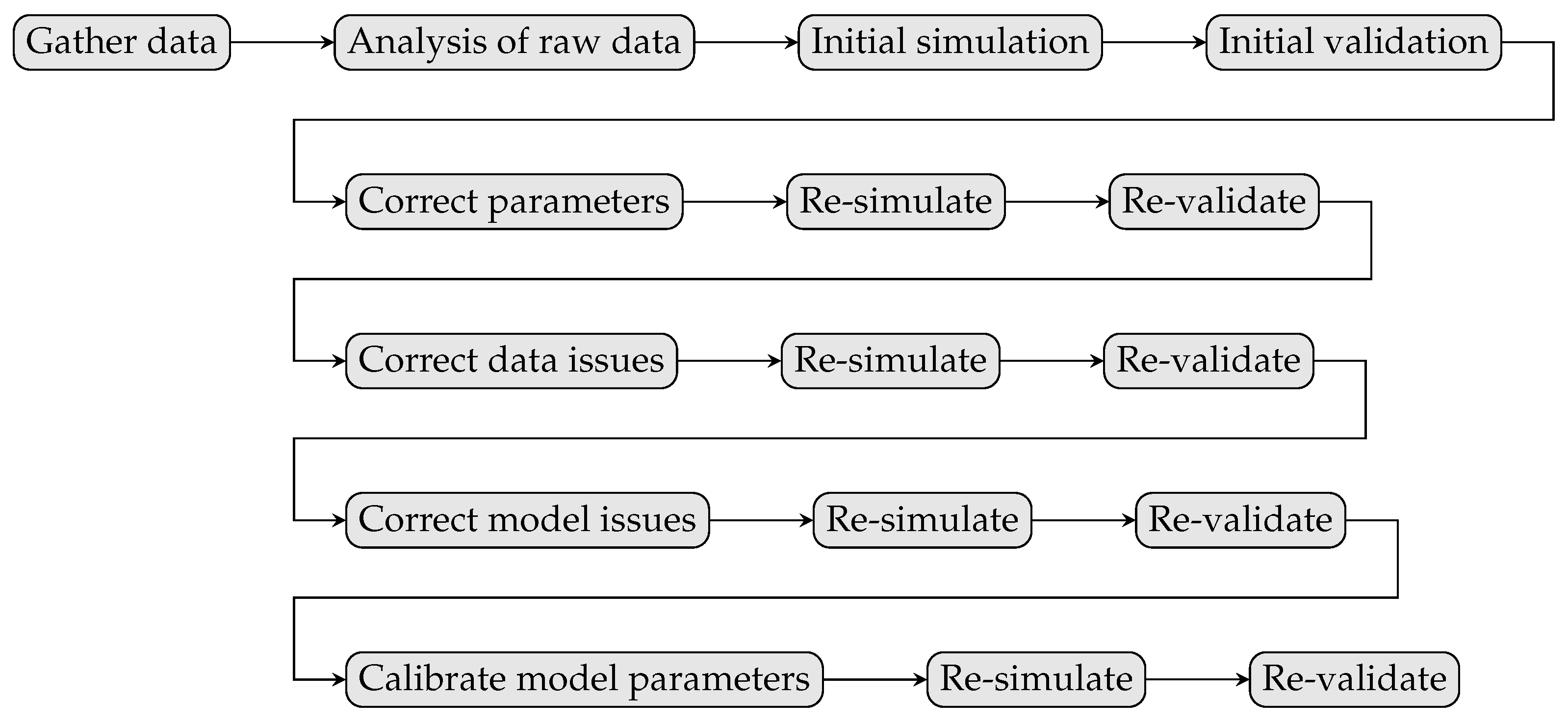
2.3. Simulation
3. Results
3.1. Measured Results
3.2. Simulated Results with Existing Model
3.2.1. Elevation Profile Correction
3.2.2. Speed Profile Correction
3.2.3. Radial Drag and Heading Angle Correction
3.2.4. Hill-Climb Force Model Correction
3.2.5. Parameter Tuning
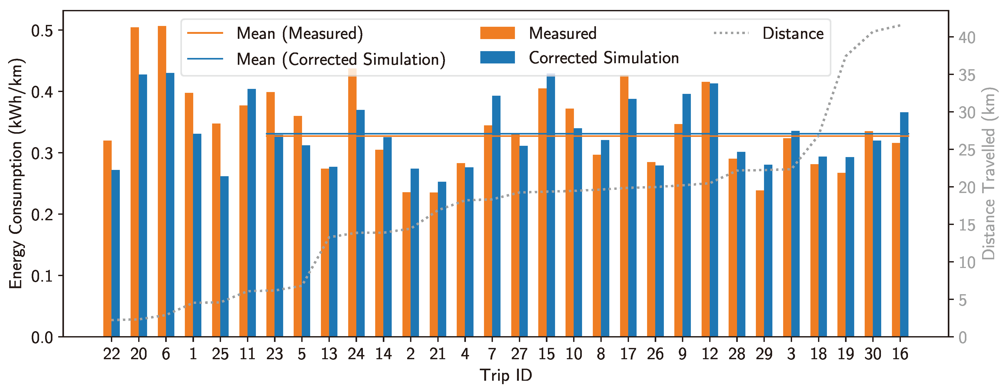
3.3. Corrected Simulation Result
4. Conclusions
Limitations and Future Work
Author Contributions
Funding
Data Availability Statement
Conflicts of Interest
References
- Sims, R.; Schaeffer, R.; Creutzig, F.; Cruz-Núñez, X.; D’Agosto, M.; Dimitriu, D.; Meza, M.J.F.; Fulton, L.; Kobayashi, S.; Lah, O.; et al. Transport. In Climate Change 2014: Mitigation of Climate Change. Contribution of Working Group III to the Fifth Assessment Report of the Intergovernmental Panel on Climate Change; Edenhofer, O., Pichs-Madruga, R., Sokona, Y., Farahani, E., Kadner, S., Seyboth, K., Adler, A., Baum, I., Brunner, S., Eickemeier, P., et al., Eds.; Cambridge University Press: Cambridge, UK; New York, NY, USA, 2014; Chapter 8; p. 603. [Google Scholar]
- Albuquerque, F.D.; Maraqa, M.A.; Chowdhury, R.; Mauga, T.; Alzard, M. Greenhouse gas emissions associated with road transport projects: Current status, benchmarking, and assessment tools. Transp. Res. Procedia 2020, 48, 2018–2030. [Google Scholar] [CrossRef]
- Odhiambo, E.; Kipkoech, D.; Hegazy, A.; Hegazy, M.; Manuel, M.; Schalekamp, H.; Klopp, J.M. The Potential for Minibus Electrification in Three African Cities: Cairo, Nairobi, and Cape Town. Volvo Res. Educ. Found. 2021. Available online: https://www.researchgate.net/profile/Jacqueline-Klopp/publication/354172918_THE_POTENTIAL_FOR_MINIBUS_ELECTRIFICATION_IN_THREE_AFRICAN_CITIES_CAIRO_NAIROBI_AND_CAPE_TOWN/links/61530758522ef665fb66d03f/THE-POTENTIAL-FOR-MINIBUS-ELECTRIFICATION-IN-THREE-AFRICAN-CITIES-CAIRO-NAIROBI-AND-CAPE-TOWN.pdf (accessed on 17 January 2025).
- Zinkernagel, R.; Evans, J.; Neij, L. Applying the SDGs to Cities: Business as Usual or a New Dawn? Sustainability 2018, 10, 3201. [Google Scholar] [CrossRef]
- Sorooshian, S. The sustainable development goals of the United Nations: A comparative midterm research review. J. Clean. Prod. 2024, 453, 142272. [Google Scholar] [CrossRef]
- Lowell, D.; Huntington, A. Electric Vehicle Market Status-Update; MJ Bradley & Associates (MJB&A): Concord, MA, USA, 2020. [Google Scholar]
- Haghani, M.; Sprei, F.; Kazemzadeh, K.; Shahhoseini, Z.; Aghaei, J. Trends in electric vehicles research. Transp. Res. Part D Transp. Environ. 2023, 123, 103881. [Google Scholar] [CrossRef]
- Motavalli, J. Every Automaker’s EV Plans Through 2035 and Beyond. Available online: https://www.forbes.com/wheels/news/automaker-ev-plans/?utm_content=196940405&utm_medium=social&utm_source=linkedin&hss_channel=lcp-19173951 (accessed on 17 January 2025).
- Rajper, S.Z.; Albrecht, J. Prospects of Electric Vehicles in the Developing Countries: A Literature Review. Sustainability 2020, 12, 1906. [Google Scholar] [CrossRef]
- Chanda, R.C.; Vafaei-Zadeh, A.; Hanifah, H.; Ashrafi, D.M.; Ahmed, T. Achieving a sustainable future by analyzing electric vehicle adoption in developing nations through an extended technology acceptance model. Sustain. Futur. 2024, 8, 100386. [Google Scholar] [CrossRef]
- Ruoso, A.C.; Ribeiro, J.L.D. The influence of countries’ socioeconomic characteristics on the adoption of electric vehicle. Energy Sustain. Dev. 2022, 71, 251–262. [Google Scholar] [CrossRef]
- Mali, B.; Shrestha, A.; Chapagain, A.; Bishwokarma, R.; Kumar, P.; Gonzalez-Longatt, F. Challenges in the penetration of electric vehicles in developing countries with a focus on Nepal. Renew. Energy Focus 2022, 40, 1–12. [Google Scholar] [CrossRef]
- Chidambaram, K.; Ashok, B.; Vignesh, R.; Deepak, C.; Ramesh, R.; Narendhra, T.M.; Usman, K.M.; Kavitha, C. Critical analysis on the implementation barriers and consumer perception toward future electric mobility. Proc. Inst. Mech. Eng. Part D J. Automob. Eng. 2023, 237, 622–654. [Google Scholar] [CrossRef]
- Dioha, M.O.; Duan, L.; Ruggles, T.H.; Bellocchi, S.; Caldeira, K. Exploring the role of electric vehicles in Africa’s energy transition: A Nigerian case study. iScience 2022, 25, 103926. [Google Scholar] [CrossRef] [PubMed]
- Agunbiade, O.; Siyan, P. Prospects of Electric Vehicles in the Automotive Industry in Nigeria. Eur. Sci. J. 2020, 16, 201. [Google Scholar] [CrossRef]
- Buresh, K.M. Impacts of Electric Vehicle Charging in South Africa and Photovoltaic Carports as a Mitigation Technique. Master’s Thesis, Stellenbosch University, Stellenbosch, South Africa, 2021. [Google Scholar]
- Kumar, A.M.; Foster, V.; Barrett, F. Stuck in Traffic: Urban Transport in Africa; World Bank Group: Washington, DC, USA, 2008; Available online: https://documents1.worldbank.org/curated/zh/671081468008449140/pdf/0Urban1Trans1FINAL1with0cover.pdf (accessed on 17 January 2025).
- Saddier, S.; Patterson, Z.; Johnson, A.; Chan, M. Mapping the Jitney network with smartphones in Accra, Ghana: The AccraMobile experiment. Transp. Res. Rec. 2016, 2581, 113–122. [Google Scholar] [CrossRef]
- Behrens, R.; McCormick, D.; Mfinanga, D. Paratransit in African Cities: Operations, Regulation and Reform, 1st ed.; Routledge: London, UK, 2015. [Google Scholar] [CrossRef]
- Ehebrecht, D.; Heinrichs, D.; Lenz, B. Motorcycle-taxis in sub-Saharan Africa: Current knowledge, implications for the debate on “informal” transport and research needs. J. Transp. Geogr. 2018, 69, 242–256. [Google Scholar] [CrossRef]
- Mccormick, D.; Schalekamp, H.; Mfinanga, D. The nature of paratransit operations. In Paratransit in African Cities: Operations, Regulation and Reform, 1st ed.; Roger, B., Dorothy, M., David, M., Eds.; Routledge: New York, NY, USA, 2016; Chapter 3; pp. 59–78. [Google Scholar]
- Evans, J.; O’Brien, J.; Ch Ng, B. Towards a geography of informal transport: Mobility, infrastructure and urban sustainability from the back of a motorbike. Trans. Inst. Br. Geogr. 2018, 43, 674–688. [Google Scholar] [CrossRef]
- Sadiq Okoh, A.; Chidi Onuoha, M. Immediate and future challenges of using electric vehicles for promoting energy efficiency in Africa’s clean energy transition. Glob. Environ. Change 2024, 84, 102789. [Google Scholar] [CrossRef]
- Pretorius, B.G.; Strauss, J.M.; Booysen, M.J. Grid and mobility interdependence in the eventual electrification of operational minibus taxis in cities in sub-Saharan Africa. Energy Sustain. Dev. 2024, 79, 101411. [Google Scholar] [CrossRef]
- Collett, K.A.; Hirmer, S.A. Data needed to decarbonize paratransit in Sub-Saharan Africa. Nat. Sustain. 2021, 4, 562–564. [Google Scholar] [CrossRef]
- Falchetta, G.; Noussan, M.; Hammad, A.T. Comparing paratransit in seven major African cities: An accessibility and network analysis. J. Transp. Geogr. 2021, 94, 103131. [Google Scholar] [CrossRef]
- Beckers, C. Energy Consumption Prediction for Electric City Buses: Using Physics-Based Principles. Ph.D. Thesis, Technische Universiteit Eindhoven, Eindhoven, The Netherlands, 2022. [Google Scholar] [CrossRef]
- Kuang, H.; Qu, H.; Deng, K.; Li, J. A physics-informed graph learning approach for citywide electric vehicle charging demand prediction and pricing. Appl. Energy 2024, 363, 123059. [Google Scholar] [CrossRef]
- Croce, A.I.; Musolino, G.; Rindone, C.; Vitetta, A. Traffic and Energy Consumption Modelling of Electric Vehicles: Parameter Updating from Floating and Probe Vehicle Data. Energies 2022, 15, 82. [Google Scholar] [CrossRef]
- Giliomee, J.H.; Booysen, M.J. Grid-Sim: Simulating Electric Fleet Charging with Renewable Generation and Battery Storage. World Electr. Veh. J. 2023, 14, 274. [Google Scholar] [CrossRef]
- Hull, C.R.; Giliomee, J.H.; Collett, K.A.; McCulloch, M.D.; Booysen, M.J. High fidelity estimates of paratransit energy consumption from per-second GPS tracking data. Transp. Res. Part D Transp. Environ. 2023, 118, 103695. [Google Scholar] [CrossRef]
- Abdelgadir, S.M.; Venter, C.J. Investigating the Operational Compatibility of Minibus Taxis in the City of Tshwane with Contemporary Electrification Technologies: A Rule-Based Approach. Threadbo-18 Conference. 2024. Available online: https://ses.library.usyd.edu.au/handle/2123/33397 (accessed on 17 January 2025).
- Liu, W.; Placke, T.; Chau, K. Overview of batteries and battery management for electric vehicles. Energy Rep. 2022, 8, 4058–4084. [Google Scholar] [CrossRef]
- Burra, L.T.; Al-Khasawneh, M.B.; Cirillo, C. Impact of charging infrastructure on electric vehicle adoption: A synthetic population approach. Travel Behav. Soc. 2024, 37, 100834. [Google Scholar] [CrossRef]
- Cignini, F.; Genovese, A.; Ortenzi, F.; Alessandrini, A.; Berzi, L.; Pugi, L.; Barbieri, R. Experimental Data Comparison of an Electric Minibus Equipped with Different Energy Storage Systems. Batteries 2020, 6, 26. [Google Scholar] [CrossRef]
- Sato, S.; Jiang, Y.J.; Russell, R.L.; Miller, J.W.; Karavalakis, G.; Durbin, T.D.; Johnson, K.C. Experimental driving performance evaluation of battery-powered medium and heavy duty all-electric vehicles. Int. J. Electr. Power Energy Syst. 2022, 141, 108100. [Google Scholar] [CrossRef]
- Collett, K.A.; Hirmer, S.A.; Dalkmann, H.; Crozier, C.; Mulugetta, Y.; McCulloch, M.D. Can electric vehicles be good for Sub-Saharan Africa? Energy Strategy Rev. 2021, 38, 100722. [Google Scholar] [CrossRef]
- Abraham, C.J.; Rix, A.; Ndibatya, I.; Booysen, M.J. Ray of hope for sub-Saharan Africa’s paratransit: Solar charging of urban electric minibus taxis in South Africa. Energy Sustain. Dev. 2021, 64, 118–127. [Google Scholar] [CrossRef]
- Giliomee, J.H.; Hull, C.R.; Collett, K.; Mcculloch, M.D.; Booysen, M.J. Simulating mobility to plan for electric minibus taxis in Sub-Saharan Africa’s paratransit. Transp. Res. Part D Transp. Environ. 2023, 118, 103728. [Google Scholar] [CrossRef]
- Abraham, C.J.; Rix, A.; Booysen, M.J. Aligned Simulation Models for Simulating Africa’s Electric Minibus Taxis. World Electr. Veh. J. 2023, 14, 230. [Google Scholar] [CrossRef]
- Tilly, N.; Yigitcanlar, T.; Degirmenci, K.; Paz, A. How sustainable is electric vehicle adoption? Insights from a PRISMA review. Sustain. Cities Soc. 2024, 117, 105950. [Google Scholar] [CrossRef]
- Ayetor, G.; Mashele, J.; Mbonigaba, I. The progress toward the transition to electromobility in Africa. Renew. Sustain. Energy Rev. 2023, 183, 113533. [Google Scholar] [CrossRef]
- Schalekamp, H.; Saddier, S. Emerging Business Models and Service Options in the Shared Transport Sector in African Cities. VREF for the Mobility and Access in African Cities (MAC) Initiative, The State of Knowledge and Research, Gothenburg; VREF: Gothenburg, Sweeden, 2020. Available online: https://vref.se/wp-content/uploads/2024/01/Schalekamp-Saddier-2020-Emerging-business-models-and-service-options-in-the-shared-transport-sector-in-African-cities-VREF.pdf (accessed on 17 January 2025).
- Jelti, F.; Allouhi, A.; Tabet Aoul, K.A. Transition Paths towards a Sustainable Transportation System: A Literature Review. Sustainability 2023, 15, 15457. [Google Scholar] [CrossRef]
- Lacock, S.; du Plessis, A.A.; Booysen, M.J. Using Driving-Cycle Data to Retrofit and Electrify Sub-Saharan Africa’s Existing Minibus Taxis for a Circular Economy. World Electr. Veh. J. 2023, 14, 296. [Google Scholar] [CrossRef]
- Kurczveil, T.; López, P.Á.; Schnieder, E. Implementation of an Energy Model and a Charging Infrastructure in SUMO. In Proceedings of the Simulation of Urban Mobility, Berlin, Germany, 15–17 May 2013; Behrisch, M., Krajzewicz, D., Weber, M., Eds.; Springer: Berlin/Heidelberg, Germany, 2014; pp. 33–43. [Google Scholar]


| Reference | Progressive Steps |
|---|---|
| Abraham et al. [38] (2021) | Contributes a simulation model, which takes typical low-frequency mobility data, upsamples it using a mobility model, and simulates it with an energy-based simulation model. |
| Hull et al. [31] (2022) | Suggests the use of high-frequency data. |
| Develops and contributes a high-frequency electro-kinetic simulation model. | |
| Giliomee et al. [39] (2023) | Suggests improvements to the mobility model (driver model and mapping) to the model used by Abraham et al. [38]. |
| Abraham et al. [40] (2023) | Implements the suggestions of Giliomee et al. [39] |
| Merges the electro-kinetic simulation model of Hull et al. [31] into EV-Fleet-Sim. | |
| Makes mathematical corrections to the electro-kinetic simulation model of Hull et al. [31]. |
| Metrics | Definition |
|---|---|
| Trip payload | The weight carried by the vehicle. Heavier loads would require more energy. |
| Trip route | A number of routes were chosen for the purpose of this experiment. These trips were intra-town (within the same town) and inter-town (between towns). The two types of routes contain different terrains and result in different mobility characteristics, which would cause different energy requirements. Inter-town trips would require more energy due to longer distances and higher average speeds, but they would require less energy per unit distance because of fewer stop–start events compared to intra-town trips. |
| Trip length | This metric quantifies the exact length travelled by the vehicle. Longer distances would require more energy. |
| Elevation delta | This metric requires the net elevation difference between the end and beginning of the trip. Ending at a higher elevation than the vehicle started would imply a higher potential energy and thus more energy drawn from the battery. |
| Sum of upward elevation deltas per unit distance | The net elevation difference is not enough to conclude the effect that elevation has on energy usage. Since energy is not perfectly conserved when climbing and descending hills, hillier terrains would require more energy. Large elevation deltas per unit distance indicate routes with hills and valleys. |
| Sum of downward elevation deltas per unit distance | See previous metric’s description. |
| Sum of absolute heading angle deltas per unit distance | The tortuousness (windiness) of a trip has a large impact on energy usage. Tortuous trips cause more energy losses due to braking and turning-friction. A larger number of heading angle deltas per unit distance indicate a more tortuous trip. |
| Mean speed | Trips taken at higher speeds require more energy to traverse due to losses to aerodynamic friction. |
| Standard deviation of speed | This metric indicates how much the speed varied. A larger standard deviation implies that more acceleration and deceleration took place during the trip. |
| Type of Refinement | Refinement Detail |
|---|---|
| Vehicle parameter updates | Gross vehicle mass updated |
| Data corrections | GPS-reported elevation smoothing |
| GPS-reported speed profile smoothing | |
| GPS-reported heading angle correction | |
| Model corrections | Hill-climb force-based model change to energy-based model |
| Model parameter calibration | Propulsion and regeneration factor calibration |
| GPS ID | Time | Latitude | Longitude | Altitude | Heading | Velocity | Energy |
|---|---|---|---|---|---|---|---|
| ⋮ | ⋮ | ⋮ | ⋮ | ⋮ | ⋮ | ⋮ | ⋮ |
| 21949 | 2024-04-23 15:27:05 | −33.984837 | 18.834373 | 135 | 237.2 | 85.1 | −8.5 |
| 21950 | 2024-04-23 15:27:06 | −33.984954 | 18.834156 | 135 | 238.1 | 84.2 | −23 |
| 21951 | 2024-04-23 15:27:07 | −33.985065 | 18.833939 | 135 | 0 | 85.1 | −7.5 |
| 21952 | 2024-04-23 15:27:08 | −33.985065 | 18.833939 | 134 | 239.5 | 84.5 | 8 |
| 21953 | 2024-04-23 15:27:09 | −33.985279 | 18.833502 | 132 | 240.7 | 83.8 | 7 |
| 21954 | 2024-04-23 15:27:10 | −33.985382 | 18.833281 | 132 | 241.5 | 83.7 | 6 |
| 21955 | 2024-04-23 15:27:11 | 33.985483 | 18.833056 | 132 | 0 | 85.0 | −20.5 |
| 21956 | 2024-04-23 15:27:12 | −33.985483 | 18.833056 | 132 | 242.5 | 84.7 | −47 |
| 21957 | 2024-04-23 15:27:13 | −33.985677 | 18.832607 | 132 | 243.1 | 84.5 | −31 |
| ⋮ | ⋮ | ⋮ | ⋮ | ⋮ | ⋮ | ⋮ | ⋮ |
| Correction | Description | Difference in Energy Consumption (%) | Impact on Simulation Accuracy |
|---|---|---|---|
| Original simulation | Original simulation before corrections with model parameters of Abraham et al. [40]: 0.530 kWh/km | – | – |
| Parameter update | The mass of the model was updated to match the physical vehicle. The mass, which was a fixed 3900 kg, was updated to a value between 2100 kg to 3000 kg, depending on how heavily the vehicle was loaded in the given trip. | Depends on the parameter being adjusted. In this case, it had a high impact on energy consumption, as mass is a highly sensitive parameter, as highlighted by Abraham et al. [40]. | |
| Elevation smoothing | Gaussian smoothing was applied to GPS elevation data. | Small, negative impact on energy consumption. High impact on power profile, as frequent power spikes due the hill-climbing are removed. | |
| Speed profile smoothing | Gaussian smoothing was applied to GPS speed data. | Medium/low, negative impact on energy consumption. Medium impact on power profile, as power spikes due to acceleration are removed. | |
| Heading angle correction | Heading angles that were falsely reset to zero by the GPS sensor were interpolated from other non-zero heading angles in order to more accurately predict the radial drag power loss. | Medium/low, negative impact on energy consumption. Medium/low impact on power profile, as power spikes due to radial drag are removed. However, these spikes are not very significant, as radial drag is a small component of the total power. | |
| Hill-climb power model correction | The hill-climb power was calculated from the change in altitude rather than from the road gradient, which was sometimes inaccurate. | Medium, negative impact on energy consumption. High impact on power profile, as frequent power spikes due the hill-climbing are removed. | |
| Parameter tuning | Propulsion and regen coefficients were tuned until the simulation accuracy was optimised. Propulsion coeff. changed from 0.90 to 0.855 and regen coeff. changed from 0.65 to 0.70 | Medium impact on energy consumption. Impact depends on how accurate the initial guess was and what parameters are tuned. | |
| Final simulation | Final simulation after all corrections were applied: 0.331 kWh/km | – | – |
Disclaimer/Publisher’s Note: The statements, opinions and data contained in all publications are solely those of the individual author(s) and contributor(s) and not of MDPI and/or the editor(s). MDPI and/or the editor(s) disclaim responsibility for any injury to people or property resulting from any ideas, methods, instructions or products referred to in the content. |
© 2025 by the authors. Licensee MDPI, Basel, Switzerland. This article is an open access article distributed under the terms and conditions of the Creative Commons Attribution (CC BY) license (https://creativecommons.org/licenses/by/4.0/).
Share and Cite
Abraham , C.J.; Lacock , S.; du Plessis, A.A.; Booysen, M.J. Empirically Validated Method to Simulate Electric Minibus Taxi Efficiency Using Tracking Data. Energies 2025, 18, 446. https://doi.org/10.3390/en18020446
Abraham CJ, Lacock S, du Plessis AA, Booysen MJ. Empirically Validated Method to Simulate Electric Minibus Taxi Efficiency Using Tracking Data. Energies. 2025; 18(2):446. https://doi.org/10.3390/en18020446
Chicago/Turabian StyleAbraham , Chris Joseph, Stephan Lacock , Armand André du Plessis, and Marthinus Johannes Booysen. 2025. "Empirically Validated Method to Simulate Electric Minibus Taxi Efficiency Using Tracking Data" Energies 18, no. 2: 446. https://doi.org/10.3390/en18020446
APA StyleAbraham , C. J., Lacock , S., du Plessis, A. A., & Booysen, M. J. (2025). Empirically Validated Method to Simulate Electric Minibus Taxi Efficiency Using Tracking Data. Energies, 18(2), 446. https://doi.org/10.3390/en18020446