Fault Location in H-Type AC Filters Based on Characteristics of Sudden Current Changes

Abstract

The timely detection and accurate location of capacitor element breakdown faults (CEBFs) are crucial in optimizing the performance of alternating current (AC) filters and ensuring the safety and stable operation of high-voltage direct current transmission systems. In this paper, by analyzing the physical process of CEBFs and the transient fault characteristics, a mapping relationship is established between the initial phase angle of the fault, the direction of sudden changes in unbalanced current, and the current difference on the low-voltage side for CEBFs occurring in different bridge arms. A fault arm localization method is developed for CEBFs in H-type AC filters based on the direction of sudden current changes. This technique is shown to enhance both the location accuracy and reliability compared with previous methods. The feasibility and accuracy of the proposed method are validated through simulations and experimental data.

1. Introduction

High-voltage direct current (HVDC) transmission systems are widely used because of their long-distance and large-capacity power transmission capabilities [1,2]. In HVDC systems, alternating current (AC) filters are key components in filtering out harmonics generated by converter devices and compensating for the reactive power absorbed during the operation of such devices. AC filters often feature high-voltage capacitor banks configured in an H-bridge arrangement [3,4,5,6] and are critical for ensuring the stable operation of power systems and improving power quality [7]. However, HVDC systems often suffer from capacitor element breakdown faults (CEBFs) relating to the AC filters due to the frequent switching operations and harsh working conditions [8]. Such faults not only affect the normal operation of the filters but also present a significant threat to the entire power system [9].

Currently, the safe operation of filter capacitor banks is typically ensured through internal element protection and external bridge differential imbalance protection [10,11]. Most capacitor units are equipped with internal fuses for isolating faulty elements. However, when a small number of elements in the capacitor break down and the fault does not reach the protection threshold [12], minor internal faults may develop into severe faults [13]. Existing imbalance protection systems in AC filters can detect severe faults by monitoring unbalanced currents and voltage deviations but are not sufficiently sensitive to a small number of element breakdowns. Therefore, the timely and sensitive monitoring and localization of CEBFs are of great significance in ensuring the safety of AC filters.

Several methods have been developed for the localization of CEBFs. Although these approaches have their merits, they primarily focus on steady-state component analysis and may have certain limitations. For instance, Mu et al. [14] determined the fault arm by analyzing the steady-state changes in unbalanced currents, terminal currents, and the currents on the high-voltage side before and after a fault. Lei et al. [15] proposed a method for identifying the fault arm using the relative steady-state currents, whereby two relative current values were calculated using two currents on the low-voltage side and the unbalanced current, and the fault arm was determined by the step change in the relative current values. Yu et al. [16] identified fault arm by calculating the quantitative relationship between unbalanced current, terminal current, and a current on the high-voltage side. Li et al. [17] introduced a method based on a probabilistic neural network for fault localization.

The existing methods outlined above can effectively locate CEBFs in filter capacitors. Certain methods require the addition of current transformers on the high-voltage side, which not only increase costs but also pose safety risks [14,16,17]. Lei et al. [15] added current transformers on the low-voltage side to reduce costs, but a reliance on steady-state components for detection renders this approach ineffective in recognizing faults when a small number of elements have broken down. In comparison, the characteristics of transient components caused by CEBFs are prominent, easy to separate, and provide more information. Exploring fault diagnosis methods based on transient features has important engineering significance [18,19,20]. In this context, this paper proposes a fault arm localization method based on the direction of sudden current changes, which requires only the addition of a single current transformer on the low-voltage side. To clearly illustrate the advantages and limitations of these methods, a comparison can be made in

Table 1. Comparison of existing fault arm localization methods.

Method	Advantages	Limitations
Steady-state variation in current [14]	Simple calculation and easy implementation	Requires additional current transformers on the high-voltage side, increasing costs and safety risks.
Relative steady-state current [15]	Simple calculation and low cost	Relies on steady-state analysis; poor performance when there are few failures of capacitor elements.
Quantitative relationship [16]	Simple calculation and easy implementation	Requires additional current transformers on the high-voltage side.
Probabilistic neural network [17]	Effectively reducing problem complexity and capable of handling complex fault scenarios	Requires additional current transformers on the high-voltage side. Requires a large amount of training data and computing resources.

.

This paper focused on the H-type AC filters of a 500-kV-line commutated, converter-based, high-voltage Direct Current (LCC-HVDC). First, the physical process and transient fault characteristics of CEBFs in H-type AC filters are analyzed, establishing a mapping relationship between the initial phase angle of the fault, the direction of sudden changes in the unbalanced current, and the current difference on the low-voltage side for different bridge arms during a fault. Subsequently, based on the direction of sudden changes, a fault arm localization method for CEBF in H-type AC filters was explained. Finally, the effectiveness of the method is verified through PSCAD/EMTDC simulations and experimental data, demonstrating its ability to accurately locate the position of each fault arm in real time. The proposed method provides a new technical approach for fault location in H-type AC filters within HVDC transmission systems.

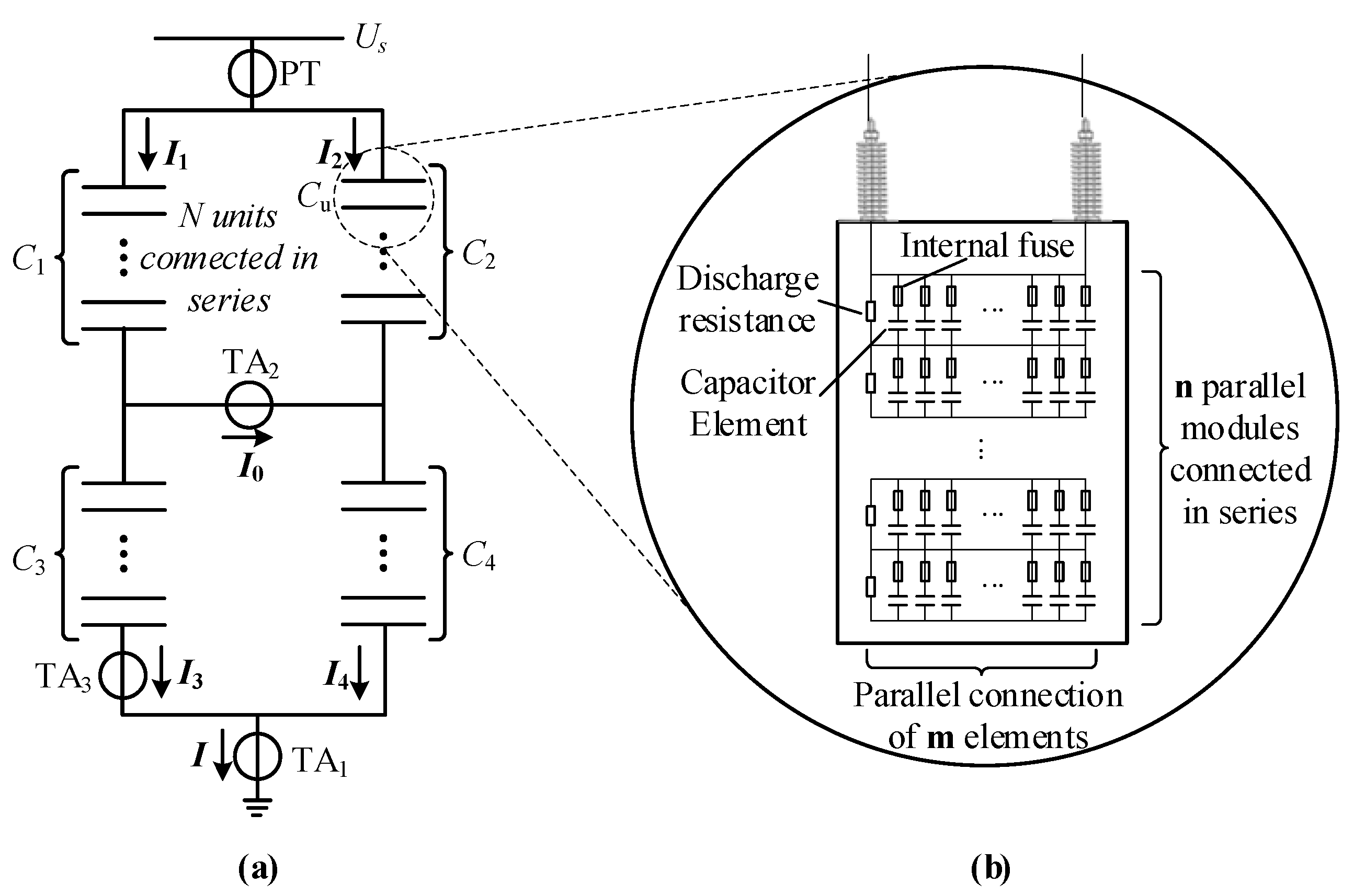
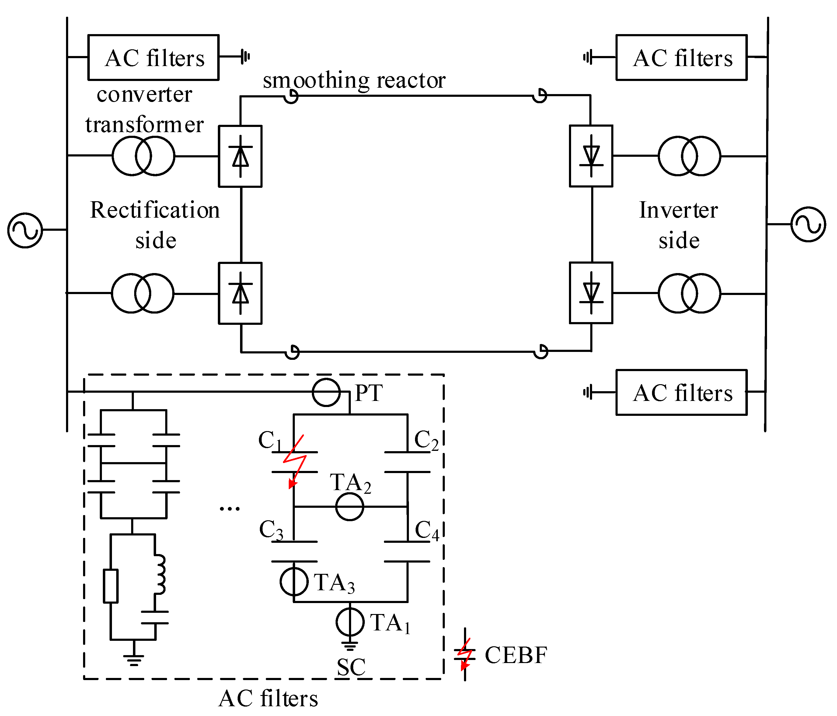
2. Equivalent Circuit and Transient Characteristic Analysis of CEBFs

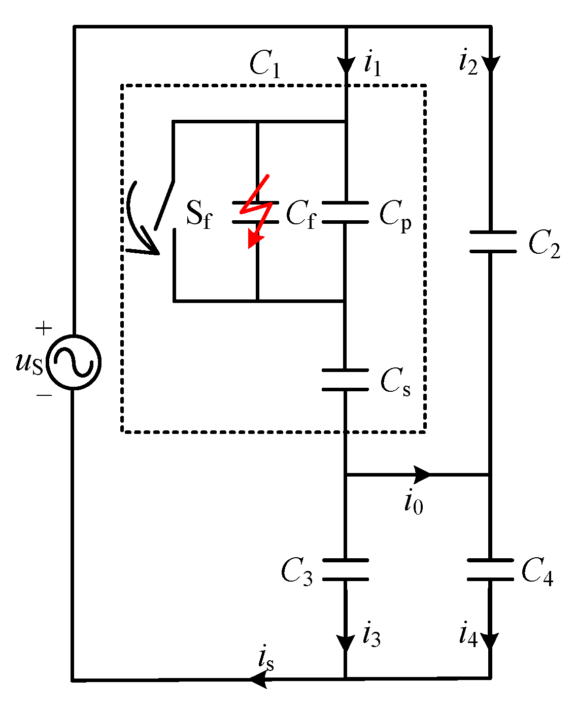
2.1. Equivalent Circuit of CEBFs

Figure 1 shows a shunt capacitor (SC) H-type AC filter [21] and its internal structure diagram. Each AC filter is composed of four bridge arms, namely C₁, C₂, C₃, and C₄. Capacitor banks C₁ and C₂ are on the high-voltage side, while capacitor banks C₃ and C₄ are on the low-voltage side. Each bridge arm consists of multiple capacitor units connected in series and parallel. The elements of the capacitor units with internal fuses generally adopt a “parallel-first, then series” connection method. In Figure 1, TA₁ is the terminal current transformer and TA₂ is the imbalance current transformer. The method proposed in this paper requires the addition of current transformer TA₃ on the low-voltage side of the H-bridge. Let each bridge arm be composed of N capacitor units connected in series, and the capacitance value of each unit be denoted as C_u. Then, C₁ = C₂ = C₃ = C₄ = C_u/N = C. Internally, each unit consists of m × n capacitor elements, where the m elements are first connected in parallel to form a parallel module, and then the n parallel modules are connected in series.

In the analysis of CEBFs, the internal fuse impedance and the lead impedance of the capacitor units are much smaller than the system impedance, so they can be neglected in the calculations [22]. In capacitor manufacturing technology, the capacitor elements generally use a protruding edge made of aluminum foil to achieve series and parallel connections. Thus, the resistance and inductance of the element lead sheets can also be disregarded [23]. Figure 2 shows the transient equivalent circuit of a CEBF, where u_S is the phase voltage and i_s the terminal current.

A certain parallel module inside a capacitor unit in bridge arm C₁ is considered to experience a CEBF at time t₀. This is equivalent to the closing of switch S_f. In Figure 2, C_f represents the capacitance value of the broken element, C_p is the equivalent capacitance value of the other elements in the same parallel module, and C_s is the equivalent capacitance value of the non-faulty series segment of the bridge arm. The following analysis focuses on the transient response caused by the CEBF.

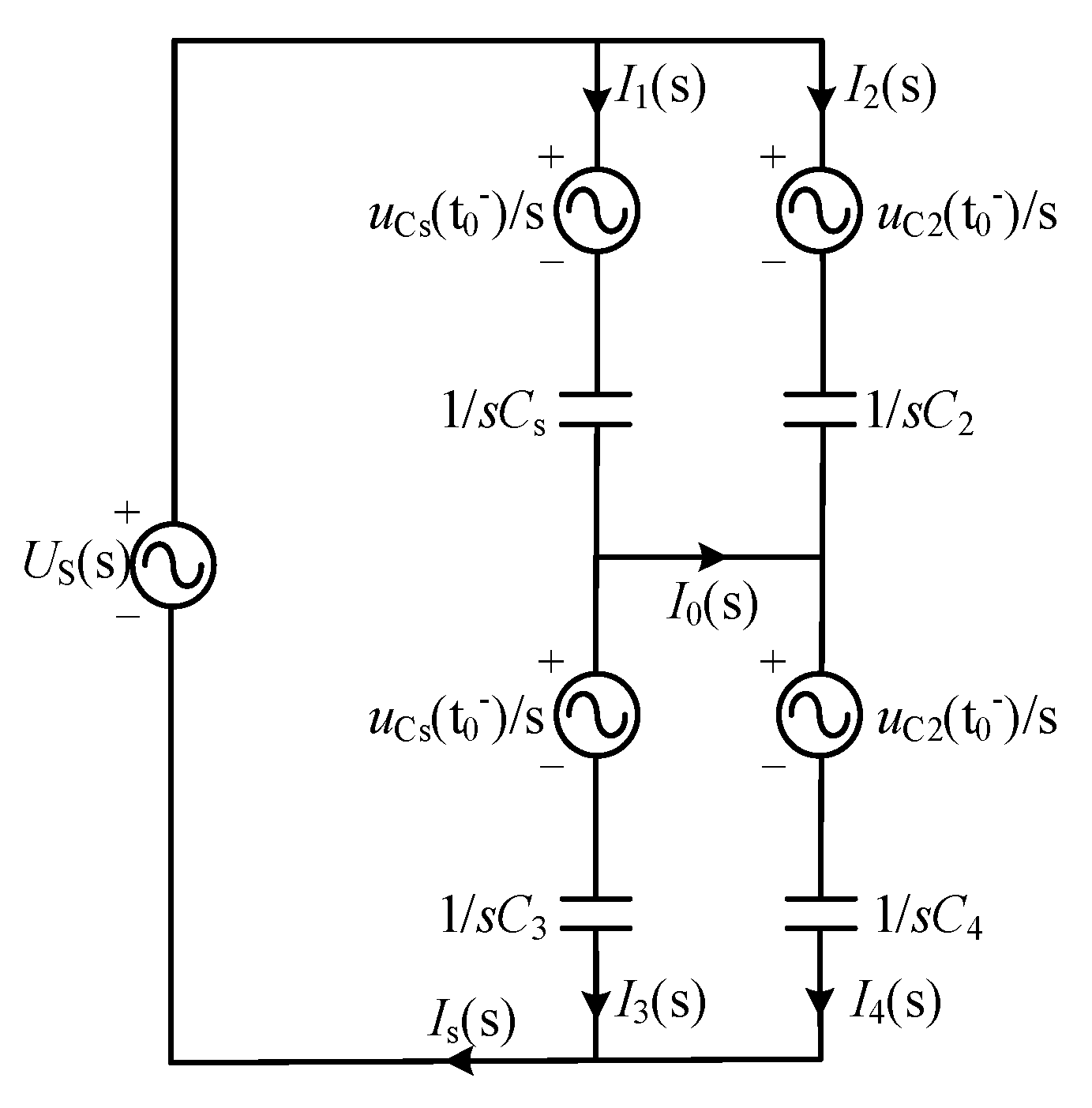
2.2. Transient Characteristic Analysis of CEBFs

The phase voltage at the moment of breakdown is $u_s(t)=U_{sm}\cos (\omega t+{\phi }_0)$, where $U_{sm}$ is the amplitude of the phase voltage, $\omega$ is the angular frequency, and ${\phi }_0$ is the initial phase angle of the fault. The s-domain expression of the phase voltage at the moment of breakdown is $U_s(s)={\displaystyle \frac{s\cos {\phi }_0-\omega \sin {\phi }_0}{s^2+{\omega }^2}}{U}_{sm}$. Before time t₀, the voltage across C_s is $u_{\mathrm{Cs}}({t_0}^{-})={\displaystyle \frac{nN-1}{2nN}}{u}_s$, n is the number of parallel modules within a capacitor unit, and N is the number of capacitor units in each bridge arm. The voltages across C₂, C₃, and C₄ are $u_{\mathrm{C}2}({t_0}^{-})=u_{\mathrm{C}3}({t_0}^{-})=u_{\mathrm{C}4}({t_0}^{-})={\displaystyle \frac{1}{2}}{u}_s$, and C₁ = C₂ = C₃ = C₄ = C, where C represents the capacitance of each bridge arm before the CEBF. At time t₀, switch S_f closes and the system is in the steady state, meaning that element C_f has broken down. The faulty parallel module (C_f + C_p) is short-circuited, and the intact element C_p in parallel with C_f will discharge to the breakdown point, followed by the fuse blowing. The equivalent model of the s-domain when t > t₀ is shown in Figure 3.

Kirchoff’s voltage law in the s-domain for Figure 3 is given by

$$\left\{\begin{array}{l}({\displaystyle \frac{1}{s{C}_s}}+{\displaystyle \frac{1}{s{C}_2}})I_1(s)-{\displaystyle \frac{1}{s{C}_2}}{I}_s(s)=-{\displaystyle \frac{U_{Cs}({t_0}^{-})}{s}}+{\displaystyle \frac{U_{C2}({t_0}^{-})}{s}}\\ ({\displaystyle \frac{1}{s{C}_3}}+{\displaystyle \frac{1}{s{C}_4}})I_3(s)-{\displaystyle \frac{1}{s{C}_4}}{I}_s(s)=-{\displaystyle \frac{U_{C3}({t_0}^{-})}{s}}+{\displaystyle \frac{U_{C4}({t_0}^{-})}{s}}\\ -{\displaystyle \frac{1}{s{C}_2}}{I}_1(s)-{\displaystyle \frac{1}{s{C}_4}}{I}_3(s)+({\displaystyle \frac{1}{s{C}_2}}+{\displaystyle \frac{1}{s{C}_4}})I_s(s)=-{\displaystyle \frac{U_{C2}({t_0}^{-})}{s}}-{\displaystyle \frac{U_{C4}({t_0}^{-})}{s}}+U_s(s)\end{array}\right..$$

(1)

Solving Equation (1) yields

$$\left\{\begin{array}{l}{I}_s(s)={\displaystyle \frac{2C(2nN-1)}{4nN-3}}s{U}_s(s)-C{U}_s(s)\\ I_0(s)={\displaystyle \frac{C}{4nN-3}}s{U}_s(s)\\ I_1(s)={\displaystyle \frac{2nNC}{4nN-3}}s{U}_s(s)-{\displaystyle \frac{C}{2}}{U}_s(s)\\ I_2(s)={\displaystyle \frac{2C(nN-1)}{4nN-3}}s{U}_s(s)-{\displaystyle \frac{C}{2}}{U}_s(s)\\ I_3(s)={\displaystyle \frac{C(2nN-1)}{4nN-3}}s{U}_s(s)-{\displaystyle \frac{C}{2}}{U}_s(s)\\ I_4(s)=I_3(s)\end{array}\right..$$

(2)

After performing an inverse Laplace transform, this can be partially expressed as

$$\left\{\begin{array}{l}{i}_0(t)={\displaystyle \frac{C{U}_{sm}\cos {\phi }_0}{4nN-3}}\delta (t_0)-{\displaystyle \frac{\omega C{U}_{sm}}{4nN-3}}\sin (\omega t-{\phi }_0)\epsilon (t_0)\\ i_3(t)-i_4(t)=0\end{array}\right.,$$

(3)

where ${\displaystyle \frac{C{U}_{sm}\cos {\phi }_0}{4nN-3}}$ is the sudden change in the unbalanced current and $-{\displaystyle \frac{\omega C{U}_{sm}}{4nN-3}}\sin (\omega t-{\phi }_0)$ is the fundamental frequency component of the unbalanced current. The current difference on the low-voltage side is given by $i_3(t)-i_4(t)$.

From Equation (3), when a CEBF occurs in bridge arm C₁ and $\cos {\phi }_0>0$, the sudden change in the unbalanced current is positive and the current difference on the low-voltage side is $i_3(t)-i_4(t)=0$, as shown in Figure 4. If $\cos {\phi }_0<0$, the sudden change in the unbalanced current is negative and the current difference on the low-voltage side is $i_3(t)-i_4(t)=0$.

Similarly, when a CEBF occurs in bridge arm C₂, the expressions for the unbalanced current and the current difference on the low-voltage side are

$$\left\{\begin{array}{l}{i}_0(t)=-{\displaystyle \frac{C{U}_{sm}\cos {\phi }_0}{4nN-3}}\delta (t_0)+{\displaystyle \frac{\omega C{U}_{sm}}{4nN-3}}\sin (\omega t-{\phi }_0)\epsilon (t_0)\\ i_3(t)-i_4(t)=0\end{array}\right.,$$

(4)

where $-{\displaystyle \frac{C{U}_{sm}\cos {\phi }_0}{4nN-3}}$ is the sudden change in the unbalanced current and ${\displaystyle \frac{\omega C{U}_{sm}}{4nN-3}}\sin (\omega t-{\phi }_0)$ is the fundamental frequency component of the unbalanced current. The current difference on the low-voltage side is given by $i_3(t)-i_4(t)$.

From Equation (4), when a CEBF occurs in bridge arm C₂ and $\cos {\phi }_0>0$, the sudden change in the unbalanced current is negative and the current difference on the low-voltage side is $i_3(t)-i_4(t)=0$, as shown in Figure 5. If $\cos {\phi }_0<0$, the sudden change in the unbalanced current is positive and the current difference on the low-voltage side is $i_3(t)-i_4(t)=0$.

When a CEBF occurs in bridge arm C₃, the expressions for the unbalanced current and the current difference on the low-voltage side are

$$\left\{\begin{array}{l}{i}_0(t)=-{\displaystyle \frac{C{U}_{sm}\cos {\phi }_0}{4nN-3}}\delta (t_0)+{\displaystyle \frac{\omega C{U}_{sm}}{4nN-3}}\sin (\omega t-{\phi }_0)\epsilon (t_0)\\ i_3(t)-i_4(t)={\displaystyle \frac{2C{U}_{sm}\cos {\phi }_0}{4nN-3}}\delta (t_0)-{\displaystyle \frac{2\omega C{U}_{sm}}{4nN-3}}\sin (\omega t-{\phi }_0)\epsilon (t_0)\end{array}\right.,$$

(5)

where $-{\displaystyle \frac{C{U}_{sm}\cos {\phi }_0}{4nN-3}}$ is the sudden change in the unbalanced current and ${\displaystyle \frac{\omega C{U}_{sm}}{4nN-3}}\sin (\omega t-{\phi }_0)$ is the fundamental frequency component of the unbalanced current. ${\displaystyle \frac{2C{U}_{sm}\cos {\phi }_0}{4nN-3}}$ is the sudden change in the current difference on the low-voltage side and $-{\displaystyle \frac{2\omega C{U}_{sm}}{4nN-3}}\sin (\omega t-{\phi }_0)$ is the fundamental frequency component of the current difference on the low-voltage side.

From Equation (5), when a CEBF occurs in bridge arm C₃ and $\cos {\phi }_0>0$, the sudden change in the unbalanced current is negative and the sudden change in the current difference on the low-voltage side is positive, as shown in Figure 6. If $\cos {\phi }_0<0$, the sudden change in the unbalanced current is positive and the sudden change in the current difference on the low-voltage side is negative.

When a CEBF occurs in bridge arm C₄, the expressions for the unbalanced current and the current difference on the low-voltage side are

$$\left\{\begin{array}{l}{i}_0(t)={\displaystyle \frac{C{U}_{sm}\cos {\phi }_0}{4nN-3}}\delta (t_0)-{\displaystyle \frac{\omega C{U}_{sm}}{4nN-3}}\sin (\omega t-{\phi }_0)\epsilon (t_0)\\ i_3(t)-i_4(t)=-{\displaystyle \frac{2C{U}_{sm}\cos {\phi }_0}{4nN-3}}\delta (t_0)+{\displaystyle \frac{2\omega C{U}_{sm}}{4nN-3}}\sin (\omega t-{\phi }_0)\epsilon (t_0)\end{array}\right.,$$

(6)

where ${\displaystyle \frac{C{U}_{sm}\cos {\phi }_0}{4nN-3}}$ is the sudden change in the unbalanced current and $-{\displaystyle \frac{\omega C{U}_{sm}}{4nN-3}}\sin (\omega t-{\phi }_0)$ is the fundamental frequency component of the unbalanced current. $-{\displaystyle \frac{2C{U}_{sm}\cos {\phi }_0}{4nN-3}}$ is the sudden change in the current difference on the low-voltage side and ${\displaystyle \frac{2\omega C{U}_{sm}}{4nN-3}}\sin (\omega t-{\phi }_0)$ is the fundamental frequency component of the current difference on the low-voltage side.

From Equation (6), when a CEBF occurs in bridge arm C₄ and $\cos {\phi }_0>0$, the sudden change in the unbalanced current is positive and the sudden change in the current difference on the low-voltage side is negative, as shown in Figure 7. If $\cos {\phi }_0<0$, the sudden change in the unbalanced current is negative and the sudden change in the current difference on the low-voltage side is positive.

In summary, the transient process caused by a CEBF is manifested as a significant sudden change in the waveform of the unbalanced current and a current difference on the low-voltage side. The sudden change is related to the bridge arm in which the CEBF is located and the initial phase angle of the fault. The specific summary is shown in

Table 2. The mapping relationship between the initial phase angle of the fault and the direction of sudden changes.

Fault Arm	The Initial Phase Angle of the Fault $\mathbf{cos}{\mathit{\phi }}_0$	The Sudden Change in the Unbalanced Current	The Sudden Change in the Current Difference on the Low-Voltage Side
C1	$\cos {\phi }_0>0$	+	0
	$\cos {\phi }_0<0$	−	0
C2	$\cos {\phi }_0>0$	−	0
	$\cos {\phi }_0<0$	+	0
C3	$\cos {\phi }_0>0$	−	+
	$\cos {\phi }_0<0$	+	−
C4	$\cos {\phi }_0>0$	+	−
	$\cos {\phi }_0<0$	−	+

.

3. Fault Location Based on Characteristics of Sudden Current Changes

When current transformers are only installed on the low-voltage side, the fault location can be accurately determined through the mapping relationship between the initial phase angle of the fault, the direction of sudden changes in unbalanced current, and the current difference on the low-voltage side. In practical systems, insufficient sampling rates mean that these impulse current components typically manifest as sudden changes in waveform and quickly return to the steady-state values after the breakdown, as shown in Figure 4, Figure 5, Figure 6 and Figure 7. To determine the location of a broken-down capacitor, it is first necessary to identify whether the breakdown was caused by a CEBF and then determine the start and end times of the sudden change process. Finally, the specific location of the CEBF is determined by calculating the initial phase angle of the fault, the unbalanced current, and the current difference on the low-voltage side during the sudden change period. The detailed steps of the proposed algorithm are as follows.

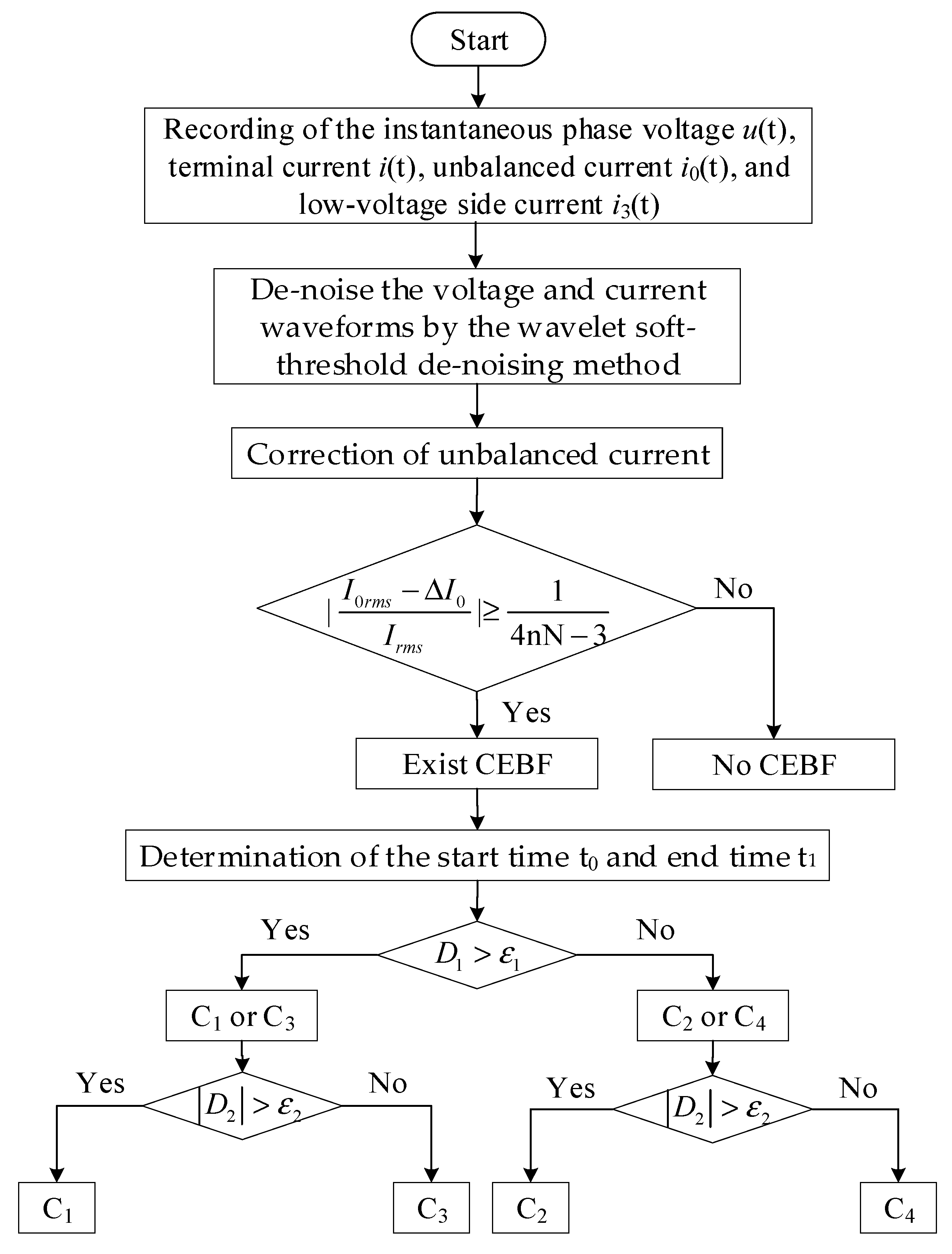
• Step 1: CEBF identification.

Correction of Unbalanced Current [24].

When an AC filter is put into operation or when a capacitor is replaced and charged for the first time, the unbalanced current needs to be corrected. At this time, the root mean square (RMS) value of the unbalanced current is recorded as the adjustment parameter ∆I₀. In subsequent calculations, the recorded adjustment parameter ∆I₀ is subtracted from the RMS value of the unbalanced current obtained from sampling to obtain the corrected unbalanced current. The RMS values of the terminal current and the unbalanced current are extracted using an RMS algorithm with a sliding point-by-point step and a calculation window of half a cycle, as described in Equation (7). Here, N_b denotes the total number of sampling points in a half-wave signal, and l and k represent the sampling sequence and the current sampling point, respectively:

$$I_{\mathrm{rms}}(k)=\sqrt{{\displaystyle \frac{1}{N_{\mathrm{b}}}}{\displaystyle \sum _{l=k-N_{\mathrm{b}}+1}^k{i}^2(l)}}.$$

(7)

Setting the Capacitor Component Breakdown Threshold [25].

When a capacitor element breaks down in C₁, the capacitance value of the C₁ bridge arm will become as shown in Equation (8).

$$C_{1\_f}={\displaystyle \frac{nN}{nN-1}}C,$$

(8)

where n is the number of parallel modules within a capacitor unit, and N is the number of capacitor units in each bridge arm. C₂ = C₃ = C₄ = C, and C represents the capacitance of each bridge arm before the fault.

The ratio of the RMS value of the unbalanced current to the RMS value of the terminal current is shown in Equation (9):

$${\displaystyle \frac{I_{0rms}}{I_{srms}}}={\displaystyle \frac{C_{1\_f}}{C_{1\_f}+C_2}}-{\displaystyle \frac{C_3}{C_3+C_4}}={\displaystyle \frac{1}{4\mathrm{nN}-2}}.$$

(9)

If there is no fault, the above value should be 0, and the ratio is independent of the system voltage. Then, considering the correction of unbalanced current, if Equation (10) is satisfied, it is CEBF.

$$\left|{\displaystyle \frac{I_{0rms}-\Delta I_0}{I_{rms}}}\right|\ge {\displaystyle \frac{1}{4\mathrm{nN}-2}}.$$

(10)

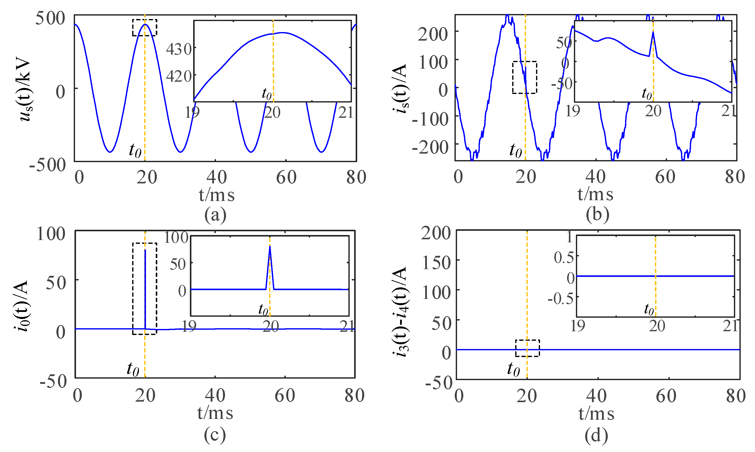
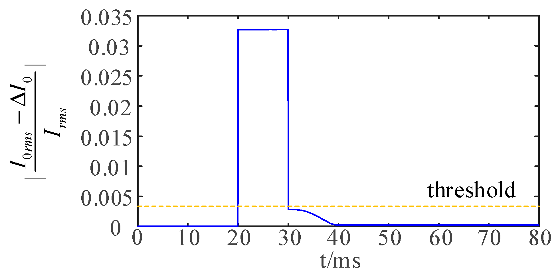
• Step 2: Determination of the start time t₀ and end time t₁ of the sudden change process.

Using the point where Equation (10) exceeds the threshold as the starting point of the sudden change process, and the corresponding time is the start time t₀ of the sudden change process. The sudden change is extremely short, so the end time t₁ of the sudden change process can be set to 0.05 ms after the start time.

• Step 3: Localization of the CEBF.

To determine the initial phase angle ${\phi }_0$ of the fault based on the fast Fourier transform, Equation (11) is used, in which a₁ and b₁ represent the amplitudes of the cosine and sine terms of the fundamental voltage component, respectively, and the sample value of the phase voltage at the k-th sampling point is denoted as u_k:

$$\left\{\begin{array}{l}{a}_1={\displaystyle \frac{1}{N}}[2{\displaystyle \sum _{k=1}^{N-1}{u}_k\cos k\frac{2\pi }{N}}]\\ b_1={\displaystyle \frac{1}{N}}[2{\displaystyle \sum _{k=1}^{N-1}{u}_k\sin k\frac{2\pi }{N}}]\end{array}\right..$$

(11)

Therefore, ${\phi }_0$ can be expressed as

$$\tan {\phi }_0={\displaystyle \frac{b_1}{a_1}}.$$

(12)

To determine the diagonal bridge arm in which the CEBF has occurred based on the direction of the sudden change in unbalanced current, the integral of the unbalanced current from time t₀ to t₁ is calculated using Equation (13). In practice, a certain current transformer error of ${\epsilon }_1=\left|0.2\%\cdot \cos {\phi }_0\cdot \max (i_0(t))\right|,t<t_0$ is considered [14].

If $D_1=\cos {\phi }_0\cdot {\displaystyle {\int }_{t_0}^{t_1}(i_0(t)-i_0(t_0))dt}>{\epsilon }_1$, the CEBF has occurred on bridge arm C₁ or C₃. If $D_1\le {\epsilon }_1$, the CEBF has occurred on bridge arm C₂ or C₄.

$${\displaystyle {\int }_{t_0}^{t_1}(i_0(t)-i_0(t_0))dt\approx {\displaystyle \sum _{k=k_0}^{k_1-1}\frac{(t_{k+1}-t_k)\cdot (i_0(t_{k+1})+i_0(t_k))}{2}}}-(t_1-t_0)i_0(t_0),$$

(13)

where k₀ and k₁ represent the sampling points corresponding to times t₀ and t₁, respectively.

To determine the specific bridge arm in which the CEBF has occurred based on the direction of the sudden change in the current difference on the low-voltage side, the integral of the current difference on the low-voltage side from time t₀ to t₁ is calculated using Equation (13). A certain current transformer error of ${\epsilon }_2=\left|0.2\%\cdot \max (2i_3(t)-i_s(t))\right|,t<t_0$ is considered.

If $\left|D_2\right|=\left|{\displaystyle {\int }_{t_0}^{t_1}(i_3(t)-i_3(t_0)-i_4(t)-i_4(t_0))dt}\right|=\left|{\displaystyle {\int }_{t_0}^{t_1}(2i_3(t)-i(t)-i(t_0))dt}\right|\le {\epsilon }_2$, the CEBF has occurred on bridge arm C₁ or C₂. If $\left|D_2\right|>{\epsilon }_2$, the CEBF has occurred on bridge arm C₃ or C₄. Combining this with the judgment from the diagonal bridge arm, the specific bridge arm in which the CEBF has occurred can be determined.

A flowchart of the CEBF localization algorithm is shown in Figure 8.

4. Simulation Verification

The accuracy of the proposed method is now verified using simulation data.

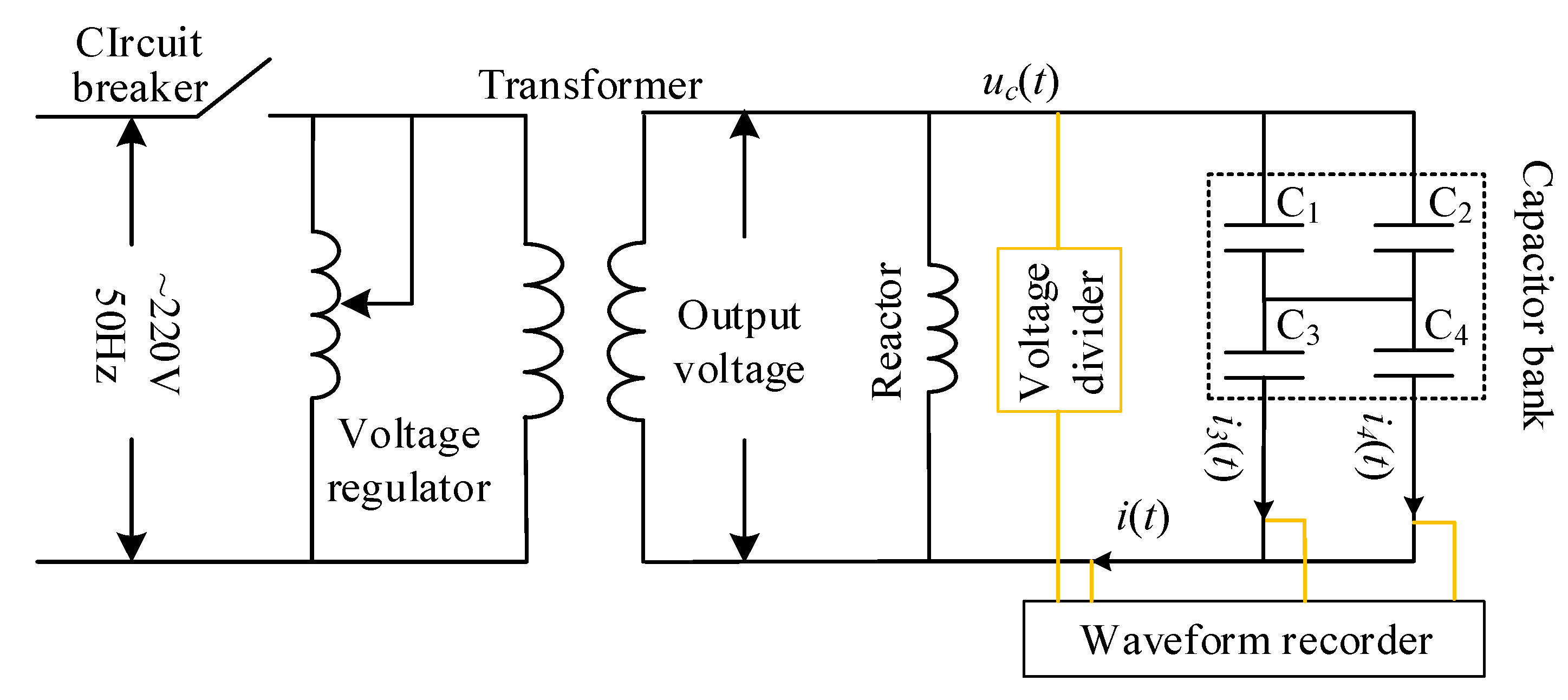
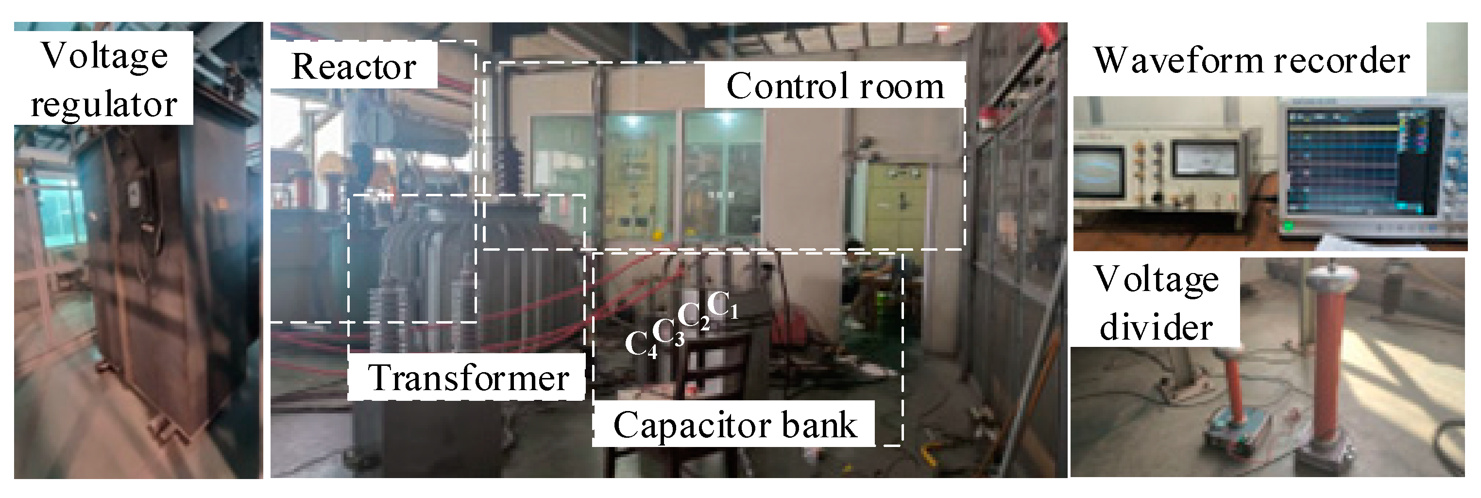
4.1. Simulation Model

A simulation model of the ±500 kV LCC-HVDC transmission system shown in Figure 9 was built in PSCAD/EMTDC [26]. To enhance the converter’s performance, the model constructs a 12-pulse converter circuit by connecting two 6-pulse converter units in series at the DC end. The main equipment of the HVDC transmission system includes a converter transformer, smoothing reactor, reactive power compensation device, AC filter, DC transmission line, and grounding system.

The bridge arm capacitor units C₁, C₂, C₃, and C₄ in AC filter capacitor bank SC have identical parameters; therefore, only the parameters of C₁ are listed here. The capacitance value of the capacitor unit is 53.8086 μF, the capacitor bank units have 1 parallel section and 30 series sections, with 15 parallel and 3 series elements within the capacitor unit.

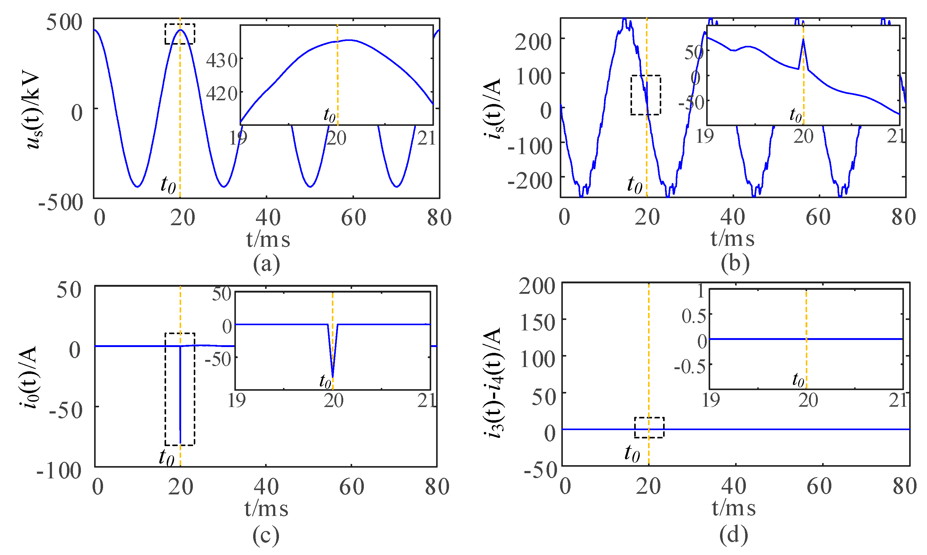
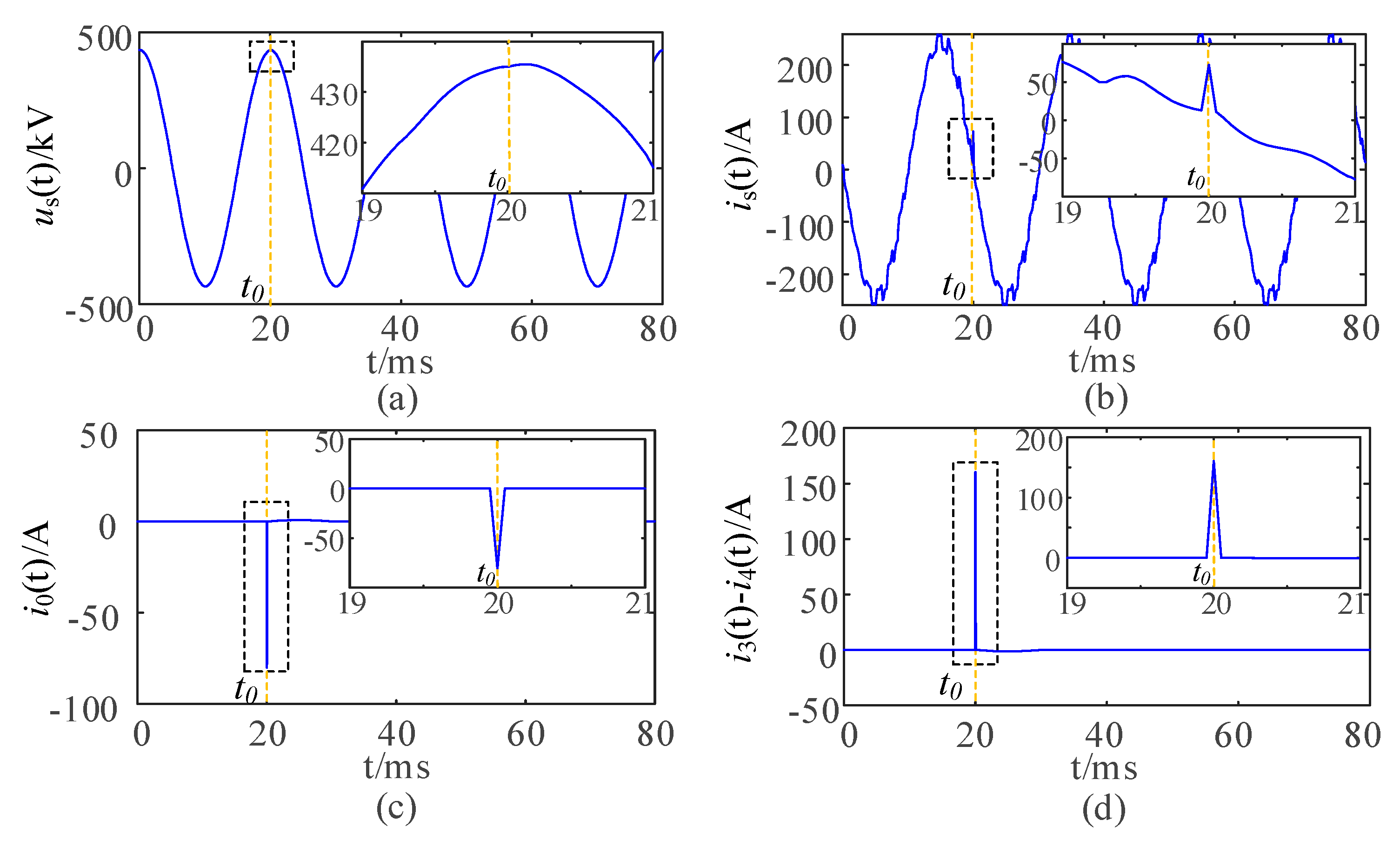
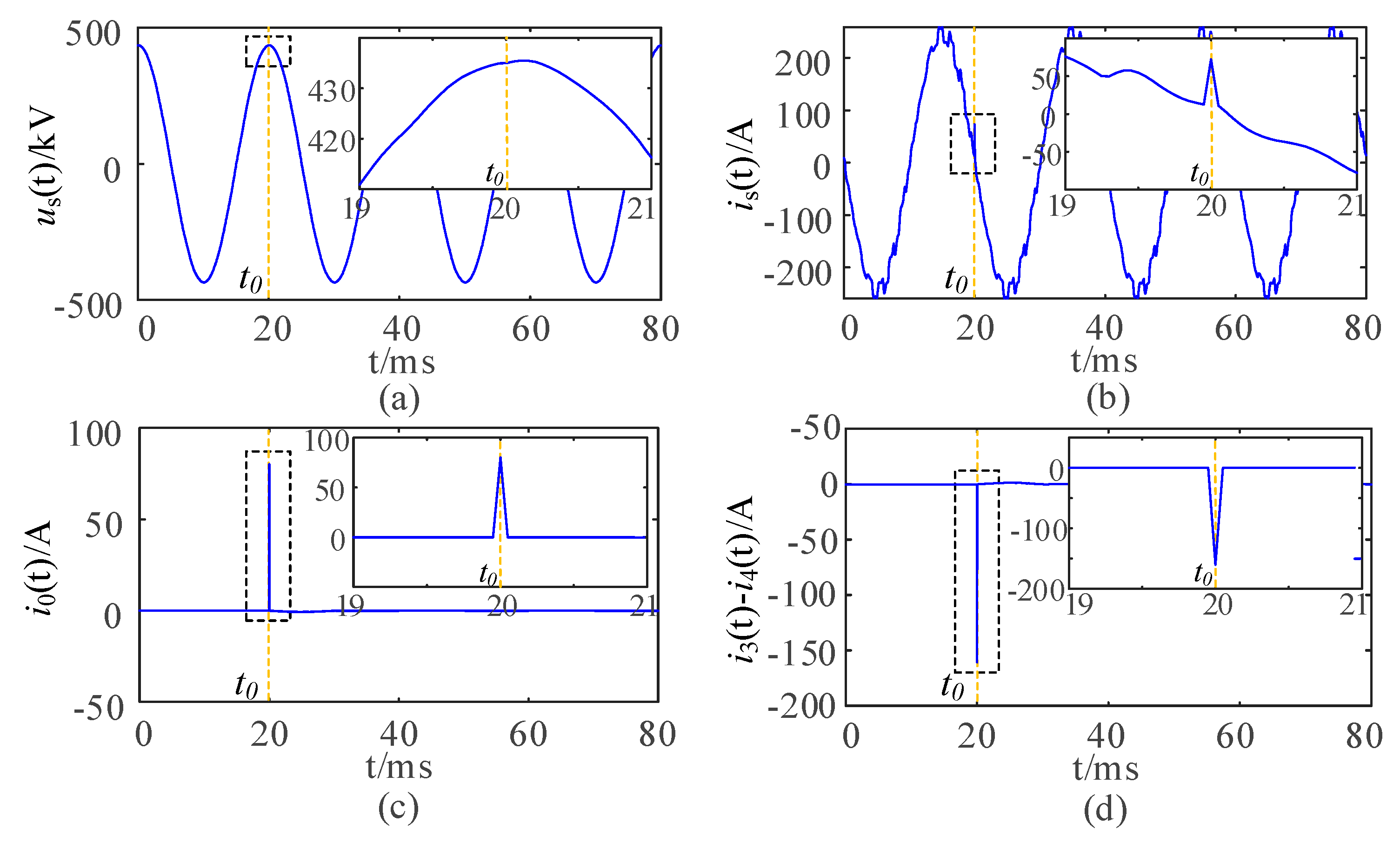
4.2. Simulation Results

Cases 1, 2, 3, and 4 represent a CEBF occurring on bridge arms C₁, C₂, C₃, and C₄, respectively. The breakdown occurs after 20 ms, at the peak of the positive half-cycle of the voltage, and the fuse blows after 20.5 ms [24]. The number of elements that break down is 1, with a capacitance value of 10.7617 µF, and the sampling frequency is 20 kHz. The proposed algorithm is verified under these conditions.

The value of $\left|{\displaystyle \frac{I_{0rms}-\Delta I_0}{I_{rms}}}\right|$ is shown in Figure 10, where the threshold is ${\displaystyle \frac{1}{4\mathrm{nN}-2}}=0.0028$. The results for all four cases are consistent, so only one case is analyzed here. The algorithm correctly identifies a CEBF.

Figure 4, Figure 5, Figure 6 and Figure 7 show the waveforms of phase voltage and currents for Case 1 to 4.

Table 3. Calculation and localization results of key feature quantities.

Fault Location	D1	D2	Localization Result
C1	1.9831	0	C1
C2	−1.9827	0	C2
C3	1.9824	3.9920	C3
C4	−1.9829	−3.9639	C4

lists the calculation and localization results of key feature quantities. These results prove that the proposed algorithm can accurately locate different faulty bridge arms.

4.3. Algorithm Influence Factor Analysis

4.3.1. The Influence of Fault Locations, Sampling Frequencies, Breakdown Times, Fuse Blowout Times, and Signal-to-Noise Ratios

Based on Figure 9, various parameter values were modified to consider the impact of different fault locations, sampling frequencies, breakdown times, fuse blowout times, and signal-to-noise ratios (SNRs) on the proposed localization method. The results in

Table 4. CEBF localization results under different influencing factors.

Fault Setting					Feature Quantities		Localization Result
Fault Location	Sampling Frequency (kHz)	Breakdown Time (ms)	Fuse Blowout Time (ms)	SNR (dB)	D1	D2
C1	15	20	0.5	100	1.9898	0	C1
	20				1.9819	0	C1
	25				1.9691	0	C1
	30				1.9617	0	C1
C2	20	15	0.5	100	−0.3039	0	C2
		20			−1.9819	0	C2
		25			−0.2599	0	C2
		30			−1.9817	0	C2
C3	20	20	0.2	100	2.0059	4.0115	C3
			0.4		2.0005	4.0011	C3
			0.6		1.9909	3.9817	C3
			0.8		1.9786	3.9573	C3
C4	20	20	0.5	40	−2.0059	−1.0118	C4
				50	−2.0060	−1.0120	C4
				60	−2.0060	−1.0119	C4
				70	−2.0058	−1.0110	C4

indicate that the faulty bridge arm can be accurately located in all cases, thus verifying the correctness of the CEBF localization algorithm for AC filters presented in this paper.

On the basis of the results in Table 4, the following conclusions can be stated.

• Sampling frequency: The sampling frequency has a significant impact on the proposed algorithm. Given that this method relies on transient signals for localization, increasing the sampling frequency significantly enhances the accuracy and reliability of the algorithm.
• Breakdown time: The breakdown time has a relatively minor impact on our method. A breakdown occurring near the voltage peak (20 ms and 30 ms) generates more significant transient current signals, while a breakdown near the voltage zero-crossing point (15 ms and 35 ms) results in smaller changes in the transient current signals.
• Fuse blowout time: The fuse blowout time has a minimal impact on the proposed algorithm. The timescale of sudden change in waveform is only 0.05 ms, which is much shorter than the time required for the fuse to blow, and the characteristic quantities used in this paper are the integral values of the sudden changes. Thus, the influence of the fuse blowout time on the algorithm is limited.
• SNR: The SNR has a minor impact on the algorithm. The localization method is based on the transient current signals, the magnitude of which is typically much greater than that of the background noise signals. Therefore, in most cases, the influence of noise on the localization accuracy is limited.

4.3.2. The Influence of Converter Type

The converter type in Figure 6 is LCC. Next, the influence of different types of converters on the proposed localization method will be discussed. First, the harmonic characteristics, filter requirements, and application scenarios of LCC, capacitor commutated converter (CCC) [27], current source converter (CSC) [28], and modular multilevel converter (MMC) [29] will be compared and analyzed, as summarized in

Table 5. Comparison of different converters.

Type of Converter	Harmonic Characteristic	Filter Requirement	Application Scenario
LCC	The 12k ± 1th order characteristic harmonics (k = 1, 2, 3, 4…)	Reactive power compensation and filtering are required	Large capacity, long-distance power transmission
CCC	The 12k ± 1th order characteristic harmonics (k = 1, 2, 3, 4…)	Need filtering	Lower requirements for power grid strength
CSC	The 12k ± 1th order characteristic harmonics with low content (k = 1, 2, 3, 4…)	Reactive power compensation and filtering are required	High requirements for commutation stability
MMC	High frequency harmonics	No need for reactive power compensation and filtering	Small and medium-sized, multi terminal DC transmission

.

Since the research object of this paper is the AC filter, the impact of different converters mainly manifests in the harmonic characteristics. Therefore, the harmonic characteristics of different converters can be compared and analyzed, and these specific harmonic characteristics can be injected into the bus voltage for equivalent simulation. This will further validate the effectiveness and applicability of the proposed method under different types of converters.

As can be seen from Table 5, the harmonic characteristics of CCC are similar to those of LCC. The principle of CCC involves directly connecting a commutation capacitor in series between the converter transformer and the converter of the LCC. This generates an additional commutation voltage across the capacitor to assist in commutation, thereby introducing additional harmonic components. Since the harmonic components generated by the commutation capacitor are very small, the CCC case is essentially the same as the LCC case.

The principle of CSC involves a second-order filter circuit composed of an inductor and capacitor connected in series on the inverter side of the LCC, which is used to eliminate harmonics generated by the converter valves. This can be equivalently represented in the simulation model of Figure 9 by reducing harmonic content on the bus to 60% and 20%, respectively, with the harmonic level of LCC as the baseline (100%).

In contrast, the harmonic level of MMC is lower, and it does not require filters or reactive power compensation devices. It can be directly represented in the simulation model of Figure 9 by reducing harmonic content on the bus to 0. The simulation results are shown in

Table 6. CEBF localization results under different converter types.

Fault Setting			Feature Quantities		Localization Result
Type of Converter	Harmonic Content (%)	Fault Location	D1	D2
LCC/CCC	/	C1	1.9819	0	C1
		C2	−1.9827	0	C2
		C3	1.9824	3.9920	C3
		C4	−1.9829	−3.9639	C4
CSC	60% LCC	C1	1.9873	0	C1
		C2	−1.9871	0	C2
		C3	1.9881	3.9962	C3
		C4	−1.9901	−3.9845	C4
	20% LCC	C1	1.9992	0	C1
		C2	−1.9985	0	C2
		C3	1.9985	3.9990	C3
		C4	−1.9983	−3.9976	C4
MMC	0	C1	2.0021	0	C1
		C2	−2.0017	0	C2
		C3	2.0020	4.0003	C3
		C4	−2.0014	−4.0011	C4

. The sampling frequency is 20 kHz, the breakdown time is 20 ms, the fuse blowout time is 0.5 ms, and the SNR is 100 dB.

The results in Table 6 indicate that the fault bridge arm can be accurately located under different types of converters, further verifying the correctness of the CEBF localization algorithm for AC filters proposed in this paper.

4.3.3. The Influence of Transformer Measurement Error

In the system shown in Figure 9, the voltage transformer with accuracy class 6P were used. For current transformers, use equipment with accuracy class 1P, 2P, and 5P, respectively. Since the measured voltage only needs to be known for its phase angle, the impact of its precision is minimal, it is not discussed further. The fault arm localization results under different transformer measurement errors are shown in

Table 7. CEBF localization results under different transformer measurement errors.

Fault Setting		Feature Quantities		Localization Result
Accuracy Class	Fault Location	D1	D2
1P	C1	1.9755	0	C1
	C2	−1.9681	0	C2
	C3	1.9722	3.9724	C3
	C4	−1.9789	−3.9408	C4
2P	C1	1.9558	0	C1
	C2	−1.9450	0	C2
	C3	1.9534	3.9371	C3
	C4	−1.9558	−3.9003	C4
5P	C1	1.9200	0	C1
	C2	−1.8800	0	C2
	C3	1.9000	3.8594	C3
	C4	−1.9115	−3.8297	C4

. The simulation results show that CEBF occurs in different bridge arms of the capacitor bank under different transformer measurement errors, and the proposed fault location scheme can accurately locate it.

4.3.4. The Influence of Capacitor Bank Configurations

For the AC filter capacitor bank SC in Figure 9, the number of capacitor units in each arm was modified, and the simulation results are shown in

Table 8. CEBF localization results under different capacitor bank configurations.

Fault Setting		Feature Quantities		Localization Result
The Number of Capacitor Units	Fault Location	D1	D2
30	C1	1.9819	0	C1
	C2	−1.9827	0	C2
	C3	1.9824	3.9920	C3
	C4	−1.9829	−3.9639	C4
60	C1	0.4970	0	C1
	C2	−0.4957	0	C2
	C3	0.4956	0.7986	C3
	C4	−0.4958	0.7928	C4
90	C1	0.2087	0	C1
	C2	−0.1992	0	C2
	C3	0.1984	0.3593	C3
	C4	−0.1998	0.3568	C4

. The simulation results indicate that the more capacitor units connected in series, the less pronounced the transient characteristics become. This is because as the number of capacitor units increases, the current change caused by the breakdown of a single element is distributed across more capacitors, thereby reducing the overall amplitude of the transient current. Additionally, with the increase in the number of capacitor units, the system’s fault tolerance improves, and the impact of a single capacitor’s failure on the overall system performance is diminished, making the transient characteristics smoother.

4.4. Comparative Analysis with Existing Methods

To demonstrate the superior performance of the proposed algorithm in fault localization, we conducted a comparative analysis with the localization methods presented in references [14,15,16,17], focusing on accuracy and speed as the key evaluation metrics. For the comparison, we randomly selected 1000 samples from the dataset that comprehensively covers the aforementioned influencing factors as the localization samples. The localization results are shown in

Table 9. Comparison of accuracy and speed of localization algorithms.

Localization Algorithm	Accuracy (%)	Average Location Time (s)
Reference [14]	85.7	0.973
Reference [15]	80.4	0.726
Reference [16]	87.0	1.131
Reference [17]	91.6	119.254
Proposed algorithm	94.6	1.467

.

As shown in Table 9, compared to the other four algorithms, the proposed algorithm achieves the highest accuracy. Its speed is slightly lower than that of [14,15,16] but outperforms [17]. This is because [14,15,16] employ simpler feature calculations, which are prone to misjudgment, while [17] utilizes a probabilistic neural network approach for localization, requiring a large number of test samples and resulting in slower speed. In summary, the proposed localization method is computationally efficient and avoids time-consuming operations.

4.5. Applicability Analysis of the Proposed Method

The method proposed in this paper achieves online fault identification and localization by adding a current transformer on the low-voltage side of the existing transformers in the AC filter, utilizing the sudden signals generated by CEBF. The simulation results show that the method exhibits strong robustness under different breakdown times, fusing times, SNRs, types of converters, transformer measurement errors, and capacitor bank configurations. The fault localization performance is particularly better when the sampling frequency is above 20 kHz, the SNR is above 40, the current transformer’s accuracy class is higher than 5P, and the number of capacitor units is less than 90.

However, implementing this method in real-world HVDC transmission systems still faces some challenges. First, the actual operating environment is subject to significant electromagnetic interference and noise, which may affect the precise capture of transient signals, especially under low SNR conditions. Additional signal processing measures are required to improve localization accuracy. Furthermore, the operating conditions of HVDC transmission systems are highly variable, such as voltage fluctuations and load changes, which may impose higher robustness requirements on the fault localization algorithm. Finally, the method requires the addition of a current transformer, and its long-term operational stability and maintenance costs are important factors to consider in practical applications.

Therefore, although the proposed method performs well in simulations, further optimization and validation are needed to address the complexity and diversity of HVDC transmission systems in real-world applications.

5. Experimental Data Verification

The experimental circuit diagram and on-site diagram are shown in Figure 11 and Figure 12, respectively. The temperature is 20 °C and the relative humidity is 57%. A CEBF experiment for the internal fuse-type capacitor bank was conducted by gradually increasing the voltage to the breakdown point, and waveform data were recorded in real-time. After the experiment, the capacitance value was measured. The parameters of the experimental devices and capacitors are listed in

Table 10. Parameters of the experimental devices.

Device	Model	Main Function	Key Parameters
Voltage regulator	TDA315	Smooth voltage regulation	Rated capacity: 315 kVA Input voltage: 380 V Output voltage: 0–650 V
Reactor	YDGK-2875/4.57−62.1	Reactive power compensation	Rated capacity: 2875 kVA SNR < 50 dB Rated frequency: 50 Hz
Transformer	EXC-315/4.57~62.1	Voltage transformation	Rated capacity: 315 kVA Rated frequency: 50 Hz
Waveform recorder	DL950	Waveform capture, data storage, waveform analysis	Number of channels: 8 Sampling Frequency ≤ 200 MHz
Voltage divider	NR-FRC-100 kV	High-voltage measurement	Voltage ratio: 100 kV

and

Table 11. Parameters of the experimental capacitors.

Capacitor	m	n	CN (uF)	C_meas (uF)	C_1st (uF)	C_2nd (uF)
C1	21	1	72	73.23	73.23	73.23
C2	21	1	72	72.46	72.46	72.46
C3	8	3	21.05	21.08	21.08	21.08
C4	8	3	21.05	20.18	19.02	open circuit

, respectively.

In Table 11, m and n denote the numbers of parallel and series elements within the capacitor unit, respectively. C_N represents the rated capacitance value, C_{_meas} is the measured capacitance value before the experiment, C_{_}1st represents the measured capacitance value after the first experiment, and C_{_}2nd represents the measured capacitance value after the second experiment.

In the first experiment, one element broke down with a sampling frequency of 1 MHz. In the second experiment, continuous breakdown faults occurred with a sampling frequency of 100 MHz. The voltage and current waveforms caused by the CEBF in the first experiment are shown in Figure 13, while the voltage and current waveforms caused by the CEBF in the second experiment are shown in Figure 14. The algorithm calculation results are shown in

Table 12. CEBF localization results.

Test Number	$\mathbf{cos}{\mathit{\phi }}_0$	D2	ε2	Localization Result
1	−0.9627	0.1732	0.0001	C4
2	0.2272	−0.3247	0.0001	C4

.

Figure 13 shows that the current difference on the low-voltage side is significant. According to Table 12, $D_2>{\epsilon }_2$ initially suggests that either C₃ or C₄ has failed. Although the on-site test conditions limited the measurement of the unbalanced current, based on the theoretical derivation, at the fault time t₀, the voltage was in the negative half-cycle, and according to the table, $\cos {\phi }_0<0$. Hence, the sudden change in the current difference on the low-voltage side was positive. Therefore, it was determined that C₄ on the low-voltage side experienced a CEBF.

Figure 14 and Table 12 illustrate that the current difference on the low-voltage side is significant, which initially suggests that either C₃ or C₄ has failed. At the fault time t₀, the voltage was in the positive half-cycle, and according to the table, $\cos {\phi }_0>0$, and the sudden change in the current difference on the low-voltage side was negative. Therefore, it was determined that C₄ on the low-voltage side experienced a CEBF. In summary, the localization result is correct.

Under the limited conditions of the experimental site, this study successfully constructed an H-type AC filter using a four-capacitor configuration and achieved resonant voltage boosting by adjusting the reactance rate of the parallel reactor. The experimental results demonstrate that the abrupt characteristics of the measured signals closely align with the simulation results, fully validating the correctness and effectiveness of the localization method proposed in this paper. It is noteworthy that, due to the use of a parallel reactor in the experiment, a noticeable oscillation phenomenon occurred during the transient process, with a longer oscillation duration compared to actual systems. In practical engineering applications, H-type AC filters typically consist of dozens or even hundreds of capacitors and do not require a parallel reactor. Although there are differences between the experimental conditions and actual systems, the experimental results still hold important reference value, providing a reliable theoretical basis for engineering applications.

6. Conclusions

This paper has addressed the fault localization problem of CEBFs in the H-type AC filters of a 500-kV LCC-HVDC and presented a fault location method based on the characteristics of sudden current changes. By analyzing the physical process and transient fault characteristics of CEBFs in H-type AC filters, a mapping relationship was established between the initial phase angle of the fault, the direction of sudden changes in the unbalanced current, and the current difference on the low-voltage side for different bridge arms during a fault. Based on the direction of sudden changes, a fault arm localization method for CEBFs in H-type AC filters was proposed. The effectiveness of this method was verified through PSCAD/EMTDC simulations and experimental data, demonstrating its ability to accurately locate the position of each fault arm in real time. The proposed method overcomes the positioning accuracy and reliability limitations of existing methods and significantly enhances the safe operation of H-type AC filters. As a supplement to existing relay protection, this method provides a new technical approach for fault location in H-type AC filters within HVDC transmission systems, offering important theoretical and engineering value.

References

1. Li, K.; Huang, M.; Zha, X. An Overview of Reliability Analysis Methods for an HVDC Transmission System. Power Syst. Prot. Control. 2024, 52, 174–187. [Google Scholar] [CrossRef]
2. Lee, J.-H.; Jung, J.-J.; Sul, S.-K. Suppression of AC Coupling Effects on HVdc Transmission System Based on MMC. IEEE Trans. Power Electron. 2024, 39, 11571–11582. [Google Scholar] [CrossRef]
3. Wang, B.; Wei, X.; Xia, Y. An Innovative Arc Fault Model and Detection Method for Circuit Breakers in LCC-HVDC AC Filter Banks. IEEE Trans. Power Deliv. 2023, 38, 3888–3899. [Google Scholar] [CrossRef]
4. Ma, X.; Yang, T.; Wang, Y.; Yuan, H.; Liu, Z.; Xu, R. Optimization Method of AC Filter Field Layout Structure in UHV Converter Station. In Proceedings of the 2023 IEEE International Conference on Power Science and Technology (ICPST), Kunming, China, 5 May 2023; pp. 173–180. [Google Scholar]
5. Huang, M.; Xiong, W.; Wu, K. Analysis of AC Filter Detuning Characteristics and Improvement Measures in Converter Station. J. Phys. Conf. Ser. 2023, 2728, 012048. [Google Scholar] [CrossRef]
6. Fanequiço, L.; Gomes, C.; Van Coller, J. Impacts of AC Filter Tripping at the Songo Rectifier Station in Southern Africa. In Proceedings of the 2024 IEEE PES/IAS PowerAfrica, Johannesburg, South Africa, 7 October 2024; pp. 1–5. [Google Scholar]
7. Gao, H. The Characteristics and Suppression Protection Measures of AC Filter Closing Inrush Current Considering Residual Voltage and Residual Charge. Eng. Lett. 2024, 32, 2191–2199. [Google Scholar]
8. Santoso, S. On Determining the Relative Location of Switched Capacitor Banks. IEEE Trans. Power Deliv. 2007, 22, 1108–1116. [Google Scholar] [CrossRef]
9. Yadav, N.; Tummuru, N.R. Filter Capacitor Current Dynamics-based Frequency-domain Fault Detection Approach for Grid-connected Low-voltage DC Microgrid. IEEE Trans. Ind. Electron. 2023, 70, 12784–12794. [Google Scholar] [CrossRef]
10. Chiradeja, P.; Lertwanitrot, P.; Ngaopitakkul, A.; Pothisarn, C. Behaviour Analysis of H-bridge High-voltage Capacitor Banks Fault on 230-kv Substation Using Discrete Wavelet Transform. IET Gener. Trans. Dist. 2023, 17, 4810–4825. [Google Scholar] [CrossRef]
11. Lertwanitrot, P.; Ngaopitakkul, A. Application of Magnitude and Phase Angle to Boundary Area-based Algorithm for Unbalance Relay Protection Scheme in 115-kV Capacitor Bank. IEEE Access 2021, 9, 35709–35717. [Google Scholar] [CrossRef]
12. Wang, Z.; Wei, L.; Yan, F.; Wu, Y.; Wang, Z.; Ma, Y. Design of the Internal Fuse Dimension for HV Shunt Capacitor in UHV Transmission Projects. IEEE Trans. Plasma Sci. 2024, 52, 2229–2240. [Google Scholar] [CrossRef]
13. Chen, X.; Yu, M.; Yin, B.; Zhao, Y.; Zhang, X.; Lv, G. Capacitor Fault Warning and Simulation Based on Harmonic Changes. Electrotech. Electric 2023, 10, 32–35. [Google Scholar]
14. Mu, D.; Lin, S.; Lei, Y.; Fang, G. Bridge Arm Fault Location Method for High Voltage Capacitor of DC Filter in HVDC Systems Based on Current Characteristics. In Proceedings of the 2020 IEEE 1st China International Youth Conference on Electrical Engineering (CIYCEE), Wuhan, China, 1 November 2020; pp. 1–7. [Google Scholar]
15. Lei, M.; Zhang, S.; Xu, X. Study on Fault Location Method of Bridge Differential Unbalanced Protection Capacitor Bank Based on Relative Current Detection. Power Capacit. React. Power Compens. 2021, 42, 1–5. [Google Scholar]
16. Yu, H.; Zhang, J.; Sun, H.; He, Y.; Zhou, H.; Yuan, M.; Yang, L.; Qu, S.; Tang, H.; Li, J. Fault Location Method of H-bridge Capacitor Bank in Converter Station Based on Current Criterion of High Voltage Bridge Arm. In Proceedings of the 2022 IEEE 5th International Conference on Automation, Electronics and Electrical Engineering (AUTEEE), Shenyang, China, 18 November 2022; Volume 2022, pp. 274–277. [Google Scholar]
17. Li, Y.; Rao, Z.; Li, Z.; Ding, L. Research on Fault Location Method of Track Circuit Compensation Capacitor Based on Probabilistic Neural Network. Electr. Meas. Instrum. 2023, 60, 48–56. [Google Scholar] [CrossRef]
18. Jouybari-Moghaddam, H.; Sidhu, T.S.; Dadash Zadeh, M.R.; Parikh, P.P. Shunt Capacitor Banks Online Monitoring Using a Superimposed Reactance Method. IEEE Trans. Smart Grid 2018, 9, 5554–5563. [Google Scholar] [CrossRef]
19. Mohanty, R.; Pradhan, A.K. Time-domain Protection and Fault Location of Wye-connected Shunt Capacitor Banks Using Superimposed Current and Differential Voltage. IEEE Trans. Power Deliv. 2021, 36, 3486–3495. [Google Scholar] [CrossRef]
20. Liang, J.; Zhu, K. Distribution Capacitor Health Monitoring Based on the Disturbances of Element Breakdown Faults. IEEE Trans. Power Deliv. 2022, 37, 4064–4072. [Google Scholar] [CrossRef]
21. Peng, Y.Z.; Wang, H.Y.; Zhang, W.N. Study on Unbalance Protection Fault of AC Filter Capacitor Bank of UHV Converter Station. Power Capacit. React. Power Compens. 2024, 6–13. [Google Scholar] [CrossRef]
22. Liang, J.B. (Shandong University, Jinan, China). Personal communication, 2021.
23. Yan, F.; He, H.W.; Wang, Z. Internal Fuse Performance of High Voltage Capacitor Unit. High Volt. Eng. 2016, 42, 1790–1796. [Google Scholar]
24. Zhu, T.-X.; Wang, N.-N.; Guo, W.-M. The Application of the Unbalance Current Protection for Capacitor of AC Filter Used in the HVDC System of CSG. Power Syst. Prot. Control. 2010, 38, 102–105. [Google Scholar]
25. Xiao, Y.; Zhang, J.Y.; Li, J.P. Criterion and Settings of Unbalanced Current Protection for Filter Capacitor Bank of H Configuration. Power Syst. Prot. Control. 2015, 43, 120–128. [Google Scholar]
26. Yan, C.; Yang, H.; Liu, Q.; Zhang, P.; Zhang, B. Impact of Nonlinear AC Fault Arc Resistance on Commutation Failures in LCC-HVDC Systems. IEEE Trans. Power Electron. 2024, 39, 12096–12100. [Google Scholar] [CrossRef]
27. Funaki, T.; Matsuura, K. Predictive firing angle calculation for constant effective margin angle control of CCC-HVdc. IEEE Trans. Power Deliv. 2000, 15, 1087–1093. [Google Scholar] [CrossRef]
28. Zhang, W.; Chen, L.; Wei, X.; Qi, L.; Gao, C.; He, Z.; Chen, Q. Design and Operation Mode of Based on Controllable Current Source Converter HVDC System. Proc. Chin. Soc. Electr. Eng. 2022, 42, 2532–2541. [Google Scholar] [CrossRef]
29. Nami, A.; Liang, J.; Dijkhuizen, F.; Demetriades, G.D. Modular multilevel converters for HVDC applications: Review on converter cells and functionalities. IEEE Trans. Power Electron. 2015, 30, 18–36. [Google Scholar] [CrossRef]
Figure 1. H-type AC filter and its internal structure: (a) AC filter; (b) capacitor unit.
Energies 18 01403 g001
Figure 2. Transient equivalent circuit of CEBF.
Energies 18 01403 g002
Figure 3. The equivalent model of the s-domain.
Energies 18 01403 g003
Figure 4. Waveform diagram when a CEBF occurs in bridge arm C1: (a) waveform of phase voltage; (b) waveform of terminal current; (c) waveform of unbalanced current; (d) waveform of the current difference on the low-voltage side.
Energies 18 01403 g004
Figure 5. Waveform diagram when a CEBF occurs in bridge arm C2: (a) waveform of phase voltage; (b) waveform of terminal current; (c) waveform of unbalanced current; (d) waveform of the current difference on the low-voltage side.
Energies 18 01403 g005
Figure 6. Waveform diagram when a CEBF occurs in bridge arm C3: (a) waveform of phase voltage; (b) waveform of terminal current; (c) waveform of unbalanced current; (d) waveform of the current difference on the low-voltage side.
Energies 18 01403 g006
Figure 7. Waveform diagram when a CEBF occurs in bridge arm C4: (a) waveform of phase voltage; (b) waveform of terminal current; (c) waveform of unbalanced current; (d) waveform of the current difference on the low-voltage side.
Energies 18 01403 g007
Figure 8. Flowchart of CEBF localization algorithm.
Energies 18 01403 g008
Figure 9. Simulation model of LCC-HVDC transmission system.
Energies 18 01403 g009
Figure 10. RMS ratio of unbalanced to terminal current.
Energies 18 01403 g010
Figure 11. Experimental circuit diagram.
Energies 18 01403 g011
Figure 12. Photographs showing on-site experimental setup.
Energies 18 01403 g012
Figure 13. Voltage and current waveforms caused by CEBF in the first experiment: (a) phase voltages caused by the CEBF; (b) magnified phase voltage after 130 ms; (c) current caused by the CEBF; and (d) magnified current after 300 ms.
Energies 18 01403 g013
Figure 14. Voltage and current waveforms caused by CEBF in the second experiment: (a) phase voltages caused by the CEBF; (b) magnified phase voltage after 15 ms; (c) current difference caused by the CEBF; and (d) magnified current difference after 15 ms.
Energies 18 01403 g014