Research on Fuel Economy of Hydro-Mechanical Continuously Variable Transmission Rotary-Tilling Tractor

Abstract

In response to the absence of an effective variable speed control strategy for tractors equipped with hydro-mechanical continuously variable transmission (HMCVT) during rotary-tillage operations, this study investigates the power transfer and fuel economy characteristics of the rotary-tilling tractor during operation. A dynamic analysis of the rotary-tilling tractor is conducted, and a dynamic model for the rotary-tilling tractor is developed. This model comprehensively incorporates factors such as the transmission efficiency of the HMCVT, the horizontal cutting force of the rotary tillage, and the torque coupling relationships between the various transmission subsystems and utilizes a backward modeling approach with dual inputs: walking load and rotary-tillage load. Based on the measured data of the effective fuel consumption rate from 64 engine groups within the study, a BP neural network model of the engine’s fuel characteristics is developed. Furthermore, it is proposed that fuel consumption per kilometer of rotary-tillage operation be used to characterize the fuel economy of the rotary-tilling tractor. The results demonstrate that the increase in forward speed concurrently enhances both the productivity and fuel economy of the rotary-tilling tractor. This finding provides a theoretical foundation for developing a variable speed control strategy for the rotary-tilling tractor.

1. Introduction

Tractors serve as both the most critical equipment in modern agricultural production and play an indispensable role in agricultural mechanization [1]. Compared to ploughing machinery, the rotary tiller offers numerous advantages, including superior soil crushing performance, enhanced soil leveling capability, and high operational efficiency. It is widely utilized in various soil environments, including plains, hills, and mountains [2]. Due to the state’s focus on the “three rural issues” and advancements in agricultural science and technology, rotary-tilling tractors equipped with traditional transmissions are no longer sufficient to meet the evolving demands of modern agricultural cultivation. As a result, these tractors continue to evolve toward large-scale, intelligent adjustments of operating parameters [3,4]. Tractors equipped with multi-stage hydro-mechanical continuously variable transmissions are capable of adapting to changes in soil conditions and fluctuations in external load. By integrating with the vehicle control strategy and continuously adjusting the transmission gear ratio, these tractors can flexibly control the unit’s operating parameters, thereby significantly enhancing the driver’s operation experience and optimizing the unit’s performance [5,6].

Developing an effective variable speed control strategy for a rotary-tilling tractor necessitates a comprehensive evaluation of the unit’s operational quality, productivity, and fuel economy [7]. In recent years, numerous scholars, have conducted extensive research on the power and economic performance of HMCVT-equipped tractors. Huang et al. [8] analyzed power loss in the transmission system and the fluctuation in the speed ratio and investigated the fuel economy variable speed control strategy of HMCVT-equipped tractors. Ahn et al. [9] developed the optimal economic operating curve for the engine and transmission by backpropagating the actual engine output based on the vehicle’s power demand to account for significant variations in transmission efficiency at different ratios. Cao et al. [10] introduced power and economy weighting coefficients and employed fuzzy inference alongside a multi-objective evolutionary algorithm based on decomposition to formulate a comprehensive mode-switching strategy, thereby enhancing tractor power and fuel economy. Zhang et al. [11] proposed a global optimal energy management strategy based on dynamic programming to enhance the energy efficiency of agricultural tractors equipped with continuously variable transmission (CVT). However, much of the previous research has focused on plowing operations, with limited exploration of rotary-tillage productivity, fuel economy, and variable speed control strategies.

The rotary tiller directly interacts with the soil, periodically performing the actions of entering, cutting, and ejecting soil. The soil exerts a significant reactive force on the blade, resulting in high total power consumption and a notable load transfer phenomenon [12,13]. Current research by scholars, primarily focuses on analyzing soil cutting resistance and power consumption in rotary-tillage knives. Bakhadir et al. [14] conducted a study based on classical mechanics to investigate the relationship between the axle torque of rotary-tillage knives and horizontal thrust in relation to changes in the rotary-tillage speed ratio. Xiong et al. [15] developed a simulation model of rotary-tiller blade–soil interaction using discrete element particle contact theory, examining the working resistance of the rotary-tiller blade in three directions. Patidar et al. [16] developed a soil–rotor blade interaction model based on the discrete element method (DEM) to analyze the effects of the ratio of rotor blade speed to tractor travel speed and the working depth on the draft and torque requirements of the rotor blades. Wang et al. [17] employed an orthogonal test method to identify the primary factors influencing the torque of rotary stubble-crushing knives and established a functional relationship between power consumption, blade speed, and plowing depth. However, most studies have concentrated on the power consumption and dynamic characteristics of the rotary tiller itself, with limited investigation into the productivity and fuel economy of rotary-tilling tractors equipped with HMCVT.

The main research contents of this paper are as follows. Taking the HMCVT-equipped LW4004 rotary-tilling tractor unit as the research object, we analyze the transmission characteristics of the rotary-tilling tractor and establish a dynamic model applicable to the rotary-tilling tractor by adopting the backward two-input modeling method. We establish a mathematical model of the engine fuel characteristics by using a BP neural network and define ‘fuel consumption per kilometer of rotary operation, G_m’ to express the fuel consumption characteristics of rotary-tilling tractor. We analyze the factors affecting the results of fuel consumption characteristics of a rotary-tilling tractor in order to provide a theoretical basis for the next step of research on the variable speed control strategy of a rotary-tilling tractor.

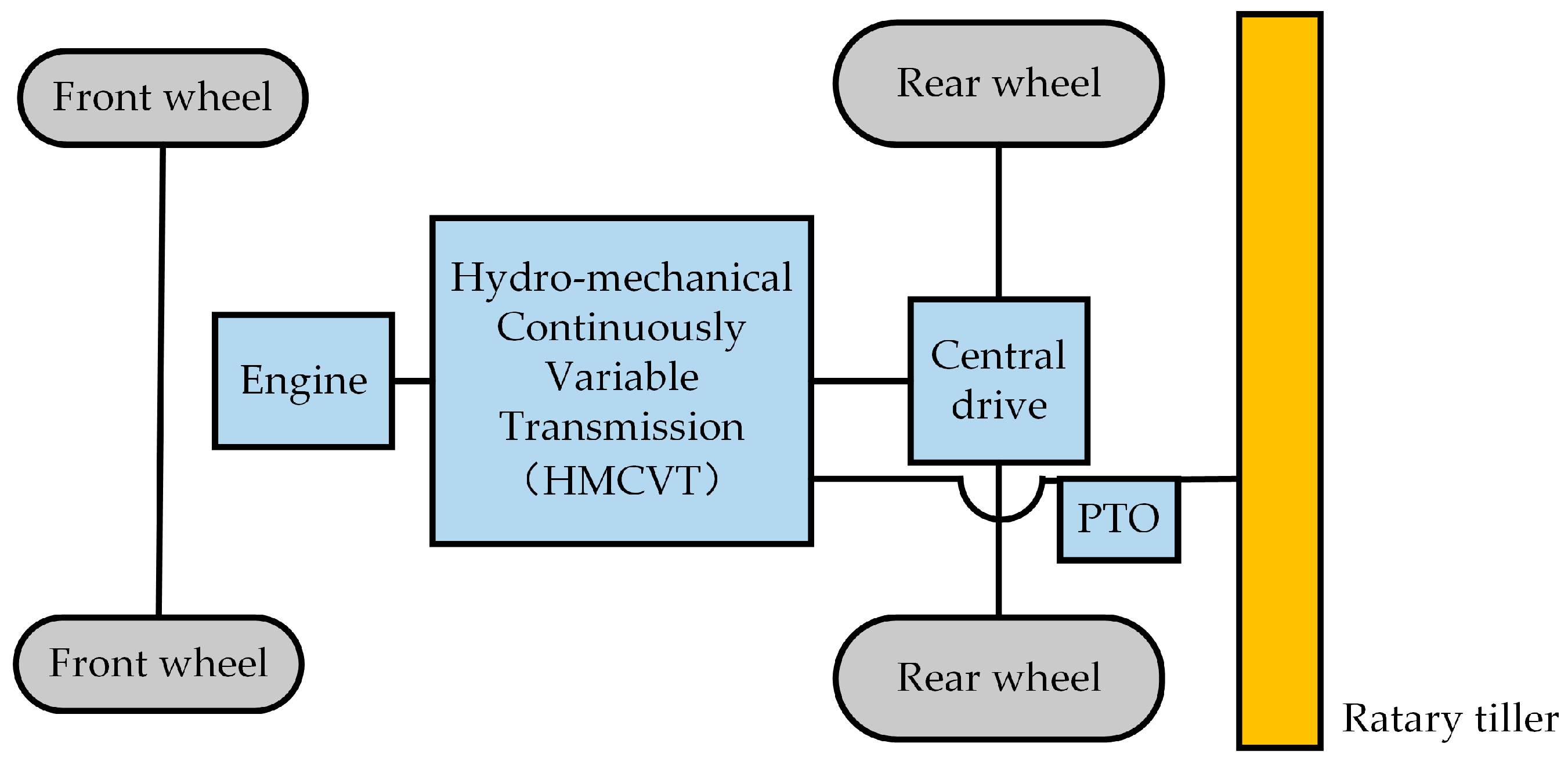
2. Transmission System Model of Rotary-Tilling Tractor

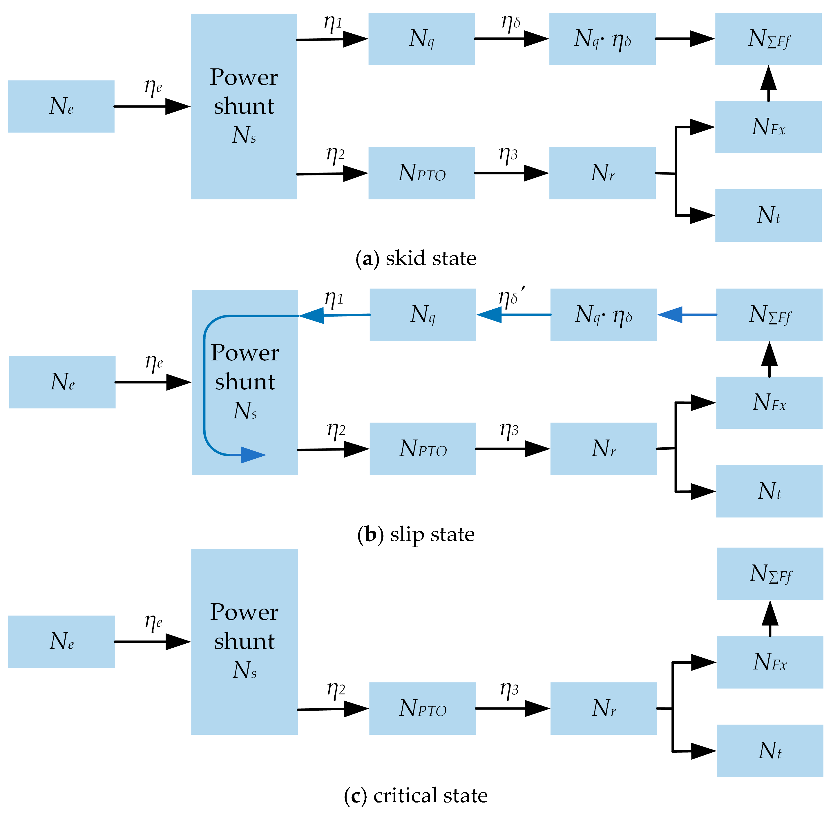
The rotary-tillage operation of a hydraulic mechanical continuously variable transmission (HMCVT) tractor relies on diesel combustion in the engine to supply energy to the machine’s power system. The engine power output is transmitted through the output shaft to the HMCVT, which then divides the power into two pathways. One pathway utilizes multi-section HMCVT speed control, transmitting power through the central drive mechanism and walking mechanism, ultimately providing energy for the tractor’s drive and traction load. The other pathway transmits power through the power take-off (PTO) and universal joints into the rotary tiller. The power is then reduced through a gearbox and transferred to the cutter shaft, ultimately providing energy for the rotary-tillage operation. Figure 1 illustrates the force analysis of the entire machine during tillage operations, while Figure 2 depicts the structure of the machine’s transmission system.

The figure defines the following parameters: G_Mm represents the weight of the unit; V_m denotes the forward speed of the unit; nr indicates the rotary speed of the cutter shaft; R_q is the radius of the tractor’s driving wheel; R refers to the rotary radius of the cutter shaft; R’ is the radius of the rotary cutter shaft torque; h is the rotary-tillage depth; F_Y1 is the support force exerted by the rear wheels of the tractor; F_Y2 is the support force exerted by the front wheels; f₁ is the rolling resistance of the rear wheels; f₂ is the rolling resistance of the front wheels; Q represents the rotary resistance; Q_x and Q_y are the horizontal and vertical components of rotary resistance, respectively; F_x is the horizontal thrust exerted by the rotary tiller on the tractor; and F_q is the driving force of the driving wheel.

Considering the power losses within the transmission system, a coupling relationship exists among the engine power and torque, the drive system, and the rotary tiller, as shown in Figure 3 and Equation (1).

The figure defines the following parameters: T_e represents the engine torque; T_q denotes the torque of the walking system’s drive shaft; T_r signifies the torque of the rotary tiller’s blade shaft; ne indicates the engine speed; n_q refers to the speed of the drive wheels; and n_r represents the speed of the rotary tiller’s blade shaft.

$$\left\{\begin{array}{l}{N}_e={\displaystyle \frac{N_q}{{\eta }_q}}+{\displaystyle \frac{N_r}{{\eta }_r}}\\ T_e={\displaystyle \frac{T_q}{{\eta }_q{i}_{e-q}}}+{\displaystyle \frac{T_r}{{\eta }_r{i}_{e-r}}}\end{array}\right.$$

(1)

where N_e represents the engine power; N_q denotes the drive power; N_r indicates the power of the rotary tiller; η_q refers to the efficiency of the drive system; η_r signifies the transmission efficiency of the rotary tiller; i_e-q denotes the transmission ratio of the drive system; and i_e-r represents the transmission ratio of the rotary-tillage system.

During operation of the rotary-tilling tractor, the horizontal and vertical components of the rotary tiller’s soil-cutting resistance in conjunction with the reaction from the three-point suspension mechanism acting on the tractor body cause the unit to experience three distinct working conditions.

(1)

When the horizontal thrust F_x of the rotary tiller is less than the total forward resistance Ff of the unit, the drive wheels require only a minimal driving force F_q to move the unit forward, resulting in a slight skid of the driving wheels.

(2)

When the horizontal thrust F_x exceeds the total forward resistance F_f, the driving force of the drive wheels drops below zero, resulting in a “braking force” F_b. In this case, the drive wheels function as braking wheels and experience slip.

(3)

When the horizontal thrust F_x equals the total forward resistance F_f of the unit, the unit is driven forward solely by the horizontal component of the rotary tiller’s force, placing it in a critical state of either no skid or slip. These three operating states are described by Equation (2).

$$\left\{\begin{array}{l}{\displaystyle \sum F_f=F_x+F_q , F_x<{\displaystyle \sum F_f}}\\ {\displaystyle \sum F_f=F_x-F_b , }{F}_x>{\displaystyle \sum F_f}\\ {\displaystyle \sum F_f=F_x , F_x={\displaystyle \sum F_f}}\end{array}\right.$$

(2)

Figure 4 illustrates the power flow analysis of the rotary-tilling tractor in three operating states.

When the unit is in the slip state, it operates in an unstable condition. The excess power generated by F_x is fed back into the drive system through the wheel-axle mechanism, leading to a parasitic power cycle. This results in additional power loss, reduced efficiency, and potential structural damage to the unit, posing safety risks.

The research focuses on the LW4004 high-power wheeled tractor with a rotary tiller from China YTO Group. This machine is equipped with a Cummins ISLe310 engine and a multi-stage HMCVT, enabling it to adapt to the complex working conditions of rotary-tillage operations. The specific parameters of the unit are provided in

Table 1. Main component parameters of rotary-tiller group of continuously variable speed tractor.

Component	Parameter	Value (Unit)
tractor	Maximum usable mass	14,000 (kg)
	Rated power	228 (kW)
	Rated speed	2100 (r/min)
	Rated torque	1200 (N·m)
	Rated tractive effort	60 (kN)
	Transmission shift	5F + 4R
	PTO rated speed	540/1000 (r/min)
	PTO Rated power	190 (kW)
	Main transmission ratio	36.348
rotary tiller	Rated power	240 (kW)
	Operation wide	4.5 (m)
	operation depth	12~26 (cm)

Note F and R represent the forward and reverse stepless transmission sections of the HMCVT, respectively.

.

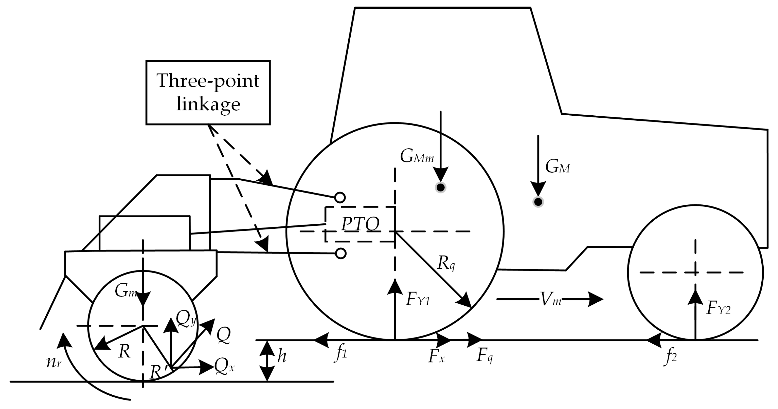
3. Dynamic Model Rotary-Tilling Tractor

3.1. Dynamic Model of Rotary Tiller

Rotary-tillage power consumption primarily results from the blade overcoming the resistance encountered during cutting, squeezing, crushing, and throwing the soil. Scholars both domestically and internationally have proposed various methods to address the issue of power consumption, including the unit method, the power method, and the resistance method. However, in actual operation, power consumption is influenced by numerous factors, such as soil conditions, rotational speed of the cutter shaft, forward speed, plowing width and depth, and blade performance and installation method. To date, no clear and easily applicable theoretical formula has been established [18].

This paper employed the simpler specific resistance method to describe the power consumption characteristics of the rotary tiller during stable operation using the following empirical formula:

$$N_r=K_{\lambda }Bh{V}_m$$

(3)

where K_λ is the soil rotary-tillage specific resistance; B is the width of rotary-tiller operation.

Rotary-tillage specific resistance is the power consumed during rotary tillage per unit volume of soil based on the determined operating parameters and soil characteristics. For a given model, assuming uniform soil conditions in the field, the rotary-tillage specific resistance is typically influenced by both the soil conditions and the rotational speed of the cutter shaft. The specific resistance will correspond to the determined soil conditions and operating parameters.

The reaction force exerted by the soil on the working parts of the rotary tiller during the cutting operation varies in both magnitude and direction across all points of the blade. The force involved in the soil cutting operation of a single blade is illustrated in Figure 5.

In the figure, α represents the angle of soil penetration during rotary tillage, β represents the angle of soil cutting, and θ is the angle between the blade and the horizontal plane, with θ = α + β.

Fang et al. [19], in their study of the force characteristics of rotary-tillage soil cutting, observed that the multidirectional resistance exerted on the blade during its motion from the initial soil contact to complete detachment varies periodically with the cutting angle of the rotary tiller. The total torque of the cutter shaft, which is the sum of the torques generated by the blades in various phases, exhibits similar periodic fluctuations. In practical operation, the knife shaft rotates at speeds of 300–400 r/min, resulting in very short fluctuation cycles. The torque fluctuations often exceed 20% of the average torque, and by using the average torque, an approximate representation of the force and torque characteristics during one rotation cycle of the rotary tiller can be derived, as shown in Equation (4)

$$\left\{\begin{array}{l}{N}_r=T_r{\omega }_r=Fv=\sqrt{F_x^2+F_y^2}v\\ F={\displaystyle \frac{T_r}{R^{\prime }}}\\ F_x=F\cos \gamma ; F_y=F\sin \gamma \end{array}\right.$$

(4)

where γ represents the angle between the resultant resistance line and the horizontal plane. According to the tractor design manual, the magnitude of γ is usually determined by the rotational radius of the knife shaft of the rotary tiller and the working depth. For deep tillage operations, the magnitude of γ is typically taken as 40° to 50° [20]. The moment of force for soil cutting by the blade is approximately R’ ≈ 0.89~0.9R. ω_r is the rotational angular velocity of the knife shaft, and v is the rotational speed of the knife shaft end point.

The absolute velocity of the blade endpoints of a forward rotary tiller during soil cutting is the resultant of the horizontal velocity in the forward direction of the unit and the circumferential velocity associated with the rotation of the cutter shaft. The equation of motion for the endpoint is derived as follows.

$$\left\{\begin{array}{l}x=v_{m}t+R\cos {\omega }_{r}t,y=R\sin {\omega }_{r}t\\ v_x=v_m-R{\omega }_r\sin {\omega }_{r}t,v_y=R{\omega }_r\cos {\omega }_{r}t\end{array}\right.$$

(5)

The absolute velocity at the end point of the blade edge is obtained as follows:

$$v=\sqrt{v_x^2+v_y^2}=\sqrt{v_m^2-2v_{m}R{\omega }_r\sin {\omega }_{r}t+R^2{{\omega }_r}^2}$$

(6)

The positive rotation of the rotary bending knife, which works perpendicular to the soil, causes the rotary plow to throw soil rearward without pushing soil behind the knife. This behavior is closely linked to the operating parameters. The conditions for the bending knife’s penetration into the soil can be expressed as follows:

$$\left\{\begin{array}{l}\lambda ={\displaystyle \frac{R{\omega }_r}{v_m}}>1\\ v_x=v\sin \alpha ={\omega }_r(R-h)>v_m\end{array}\right.$$

(7)

where λ represents the rotational speed ratio of the rotary tiller.

Since the horizontal component of the blade’s speed upon ground entry exceeds the forward speed of the unit, the direction of the horizontal component force is always aligned with the unit’s direction of travel, resulting in a thrust force acting on the unit. The vertical component force induces load transfer in the vertical direction; however, the direction of action of the blade’s vertical force before and after ground contact is opposite, with their magnitudes being nearly equal, leading to a minimal net combined force. Consequently, the effect of load transfer due to the vertical component force is disregarded. This study focused solely on the horizontal resistance, which had the greatest impact on the unit.

The relationship between rotary-tillage specific resistance, cutter shaft torque, and horizontal thrust was examined. By decoupling the actual cutter shaft torque from the operational parameters of the engine, transmission, and other systems of the unit, the soil rotary-tillage specific resistance under working conditions can be derived from Equations (3) and (4).

3.2. Soil–Tire Drive Model

Drive wheels are influenced by tire and ground conditions. Numerous studies have demonstrated that tire load, tire parameters, and soil properties are the three primary factors impacting the rolling resistance of tractor tires. A soil–tire drive model is established using a ground mechanics approach based on the soil cone index [21].

The cone index fluctuates with soil conditions, with sandy and other relatively soft soils exhibiting a lower cone index, while clay soils and uncultivated stubble fields, which are firmer, display a higher cone index. The tire index, C_n, is used to represent tire performance in contact with soil and is expressed as follows:

$$C_n={\displaystyle \frac{C_{I}bd}{F_z}}$$

(8)

where C_I is the soil cone index, kPa; b is the tire section width, mm; d is the tire diameter, mm; and F_z is the tire normal load, kN.

Given the relatively large vertical load exerted by the tractor, tire deformation occurs upon contact with the soil. To adjust the tire index, the tire maneuverability index B_n is introduced. The expression is as follows:

$$B_n=C_n{\displaystyle \frac{1+5d_{△}/h}{1+3b/d}}$$

(9)

where d_Δ is the radial deformation of the tire, mm; h is the tire section height, mm.

The rolling resistance coefficient is defined as the ratio of the tire’s rolling resistance to its vertical load and is a function of both the tire maneuverability index and the slip ratio. It can be expressed as follows:

$$\mu ={\displaystyle \frac{f}{F_z}}={\displaystyle \frac{1.2}{B_n}}+0.03+{\displaystyle \frac{0.5\sigma }{\sqrt{B_n}}}$$

(10)

where μ is the coefficient of tire rolling resistance; f is the tire rolling resistance, kN; and σ is the tire slip ratio.

Under typical operating conditions of the rotary-tilling tractor, the rolling resistance coefficient is determined based on the soil conditions encountered during rotary tillage. In uncultivated stubble fields, it typically ranges from 0.08 to 0.10; in cultivated land, from 0.12 to 0.16; and in land prepared for sowing post-plowing, from 0.16 to 0.18.

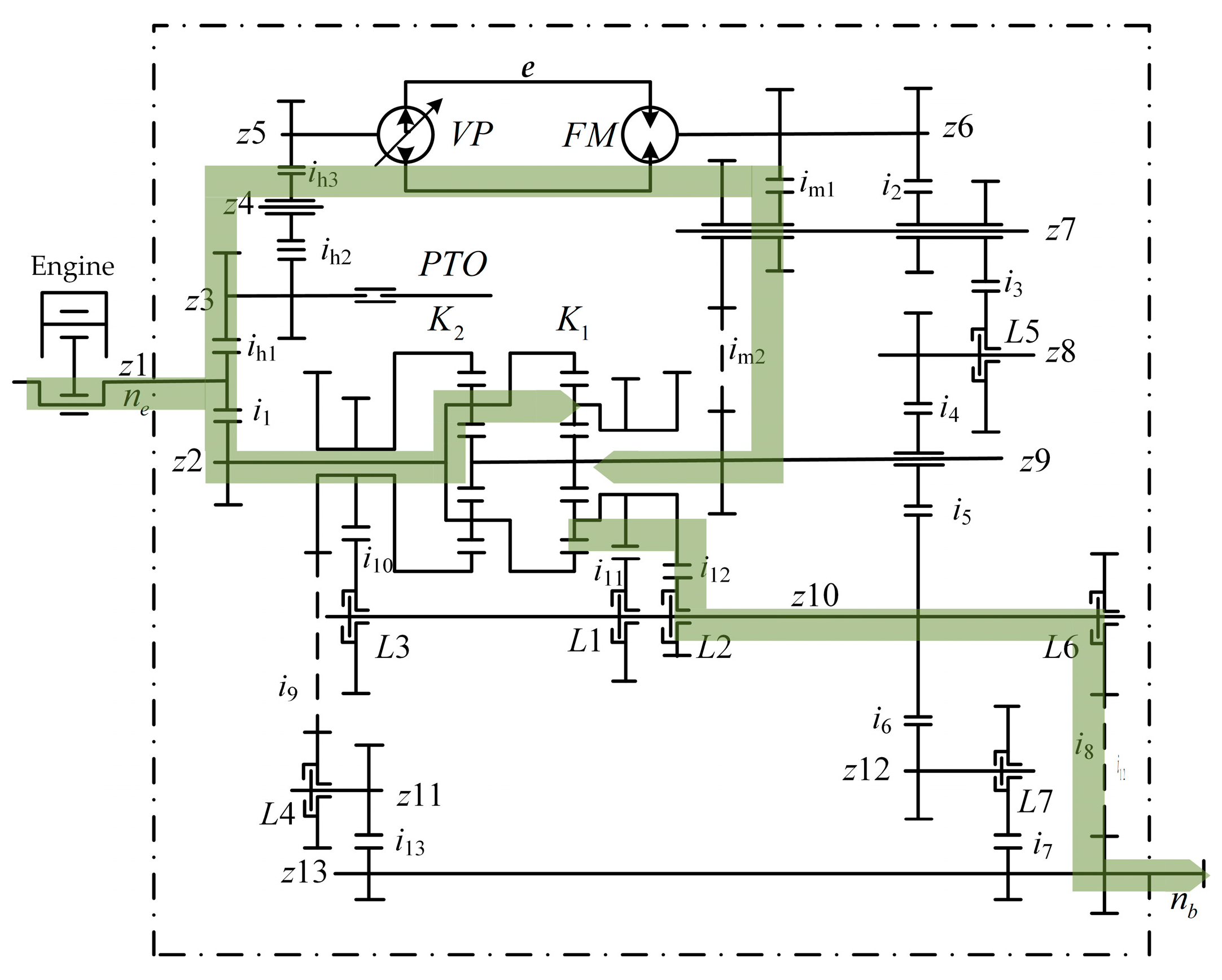
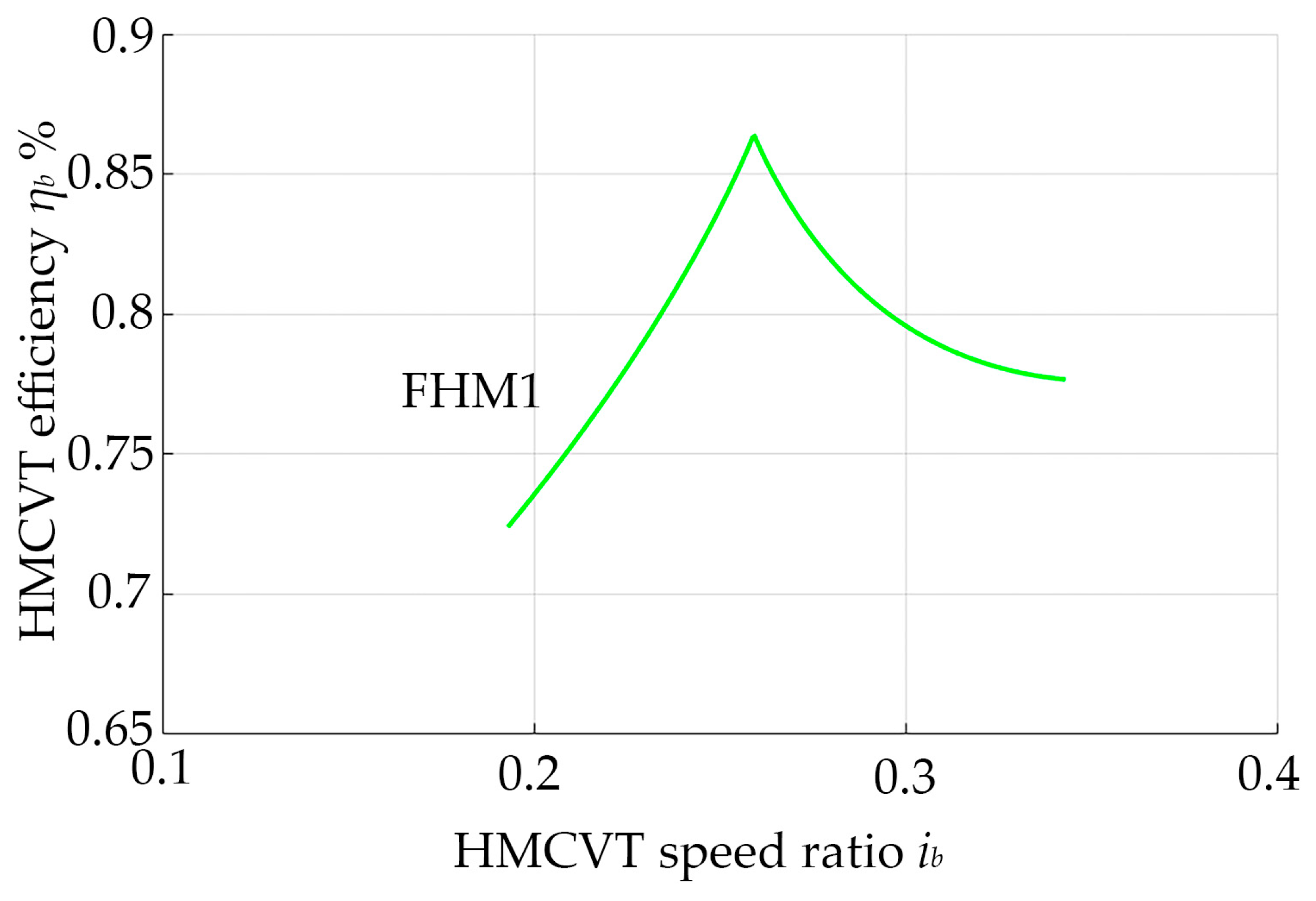
3.3. The Transmission Efficiency Characteristics of Multiple HMCVT Systems

The power transmitted to the HMCVT is divided through the gears, flowing through the pump-motor system, passing into the mechanical transmission, and ultimately outputting after converging through the planetary system. For example, the transmission principle of the LW4004 tractor equipped with a HMCVT is illustrated in Figure 6.

The multi-stage HMCVT is a closed planetary transmission, and the meshing power method is typically employed to calculate its efficiency [22]. However, in previous studies on tractor plowing conditions, the engine power flows only into the HMCVT without any power shunting. Therefore, the efficiency η_b of the HMCVT can be directly calculated from the engine output speed ω_e, torque T_e, and the HMCVT variable speed ratio i_b, but this method is not suitable for rotary-tillage operations, where power shunting is involved. To determine the HMCVT efficiency under rotary-tillage conditions, it is necessary to first calculate the output torque Tout of the transmission, as expressed in Equation (11).

$${\eta }_b=f_b(T_{out},{\omega }_e,i_b)$$

(11)

The analysis showed that during rotary-tillage operations, there was no traction resistance, and the rotary tiller generated thrust on the body. As a result, the driving force demand for the drive wheels was relatively low compared to plowing operations, keeping the drive wheel slip rate at a very low level.

3.4. Efficiency of Traveling Mechanism

The efficiency of a rotary-tillage travel system is primarily concerned with skid efficiency. Skid efficiency is generally regarded as a function of the driving force; the higher the driving force of the wheel, the greater the skid-rate and the lower the slip efficiency. The skid-rate expression is derived using test data under specific operating conditions. An expression for the skid-rate was derived from test data examining the relationship between traction force and skid-rate.

$$\delta =-{\displaystyle \frac{\ln \left(1-\frac{1}{66}(P_q-1.7161)\right)}{0.1307}}$$

(12)

As observed in the analysis, during rotary-tillage operations, the absence of traction resistance, coupled with the thrust exerted by the rotary tiller on the tractor, resulted in a relatively low demand for driving force from the drive wheels compared to conventional plowing, leading to a minimal slip rate of the drive wheels.

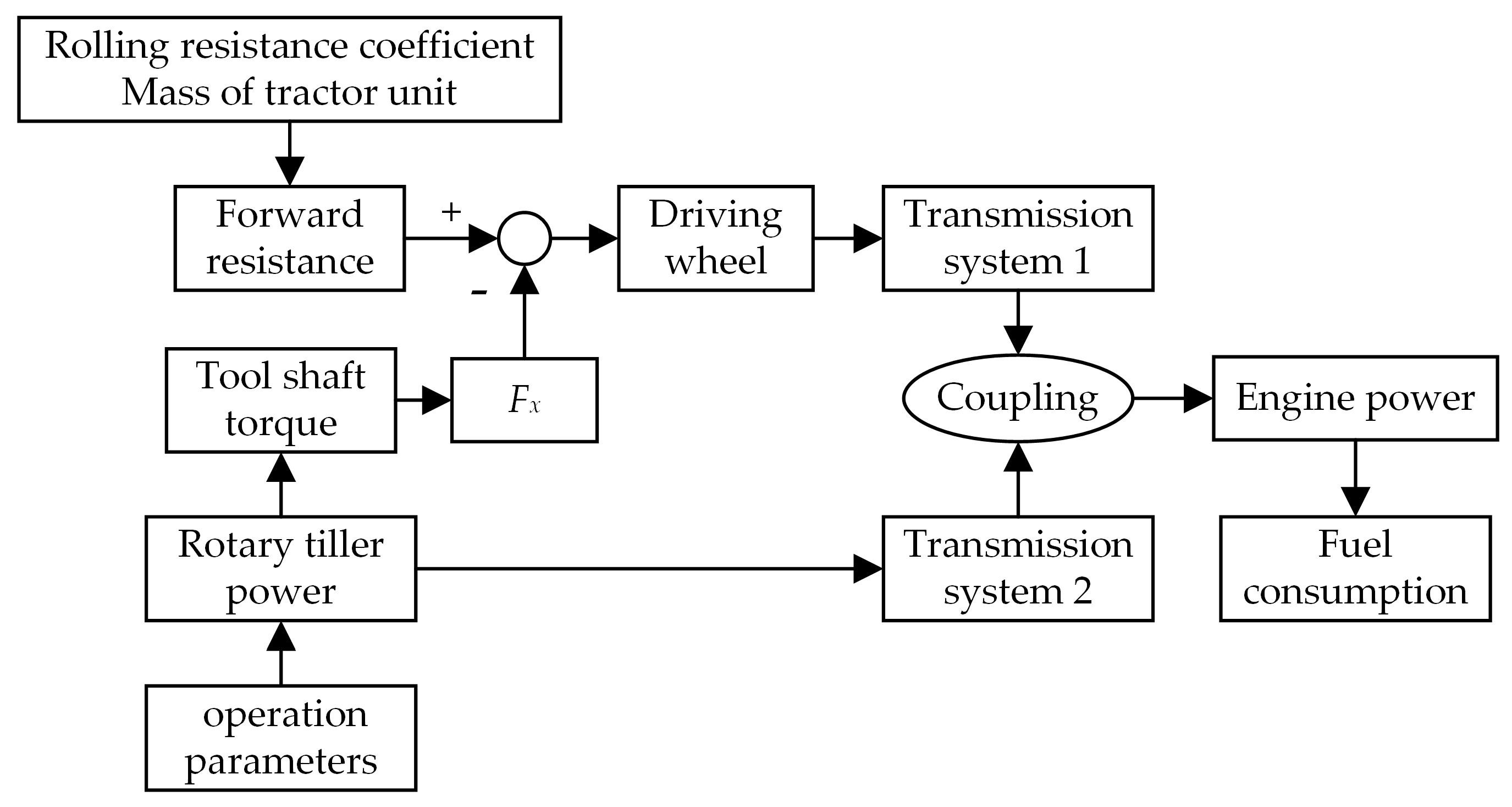
4. Modeling of the Whole Machine Transmission System

4.1. Modeling of the Overall Transmission System of the Rotary-Tilling Tractor

Three primary methods are commonly employed to calculate the power and fuel consumption of vehicles: forward modeling, backward modeling, and a hybrid approach combining both forward and backward modeling techniques [23,24]. A rotary-tilling tractor, characterized by low traveling speed, high operational power consumption, and complex and variable working conditions, has its engine power determined by the load. Given the power shunting characteristics of the unit and considering the dynamic properties of the rotary-tilling tractor, this paper utilized the backward modeling approach, incorporating dual inputs from both the walking drive load system and the implement load system, to investigate the dynamic behavior of the entire rotary-tilling tractor.

Based on the coupling relationship between the power systems illustrated in Figure 7, the power and torque coupling equations for the rotary-tilling tractor were derived, as presented in Equation (13).

$$\begin{array}{l}{N}_e={\displaystyle \frac{[\mu (M+m)g-F_x]v_m}{{\eta }_b{\eta }_z}}+{\displaystyle \frac{N_r}{{\eta }_r}}\\ T_e={\displaystyle \frac{[\mu (M+m)g-F_x]r_q}{{\eta }_b{\eta }_z{i}_{e-q}}}+{\displaystyle \frac{T_r}{{\eta }_r{i}_{e-r}}}\end{array}$$

(13)

The unit was set to operate at the engine’s rated speed and PTO 1000 rpm under standard conditions, with a forward speed ranging from 3 to 6 km/h. The plowing width and depth were set to 4.5 m and 0.18 m, respectively. In this case, the soil rotary-tillage resistance typically ranged between 30 kN and 60 kN. The rolling resistance coefficient of the soil tires was 0.18, and the transmission efficiency (η_r) of the rotary tiller was approximately 0.9 during deep tillage operations. Using the rotary-tillage resistance ratio and the forward speed of the unit as input variables, a load characteristic field for the rotary-tilling tractor during ripe land operation was established. The variation in engine power is illustrated in Figure 8.

As shown in the figure, variations in efficiency at different operating points of the HMCVT exerted a more pronounced influence on the overall power output of the ma-chine. At a constant engine speed, as the unit’s forward velocity increased, the overall power consumption correspondingly rose; thus, the primary constraint on the unit’s productivity was the engine’s maximum load capacity.

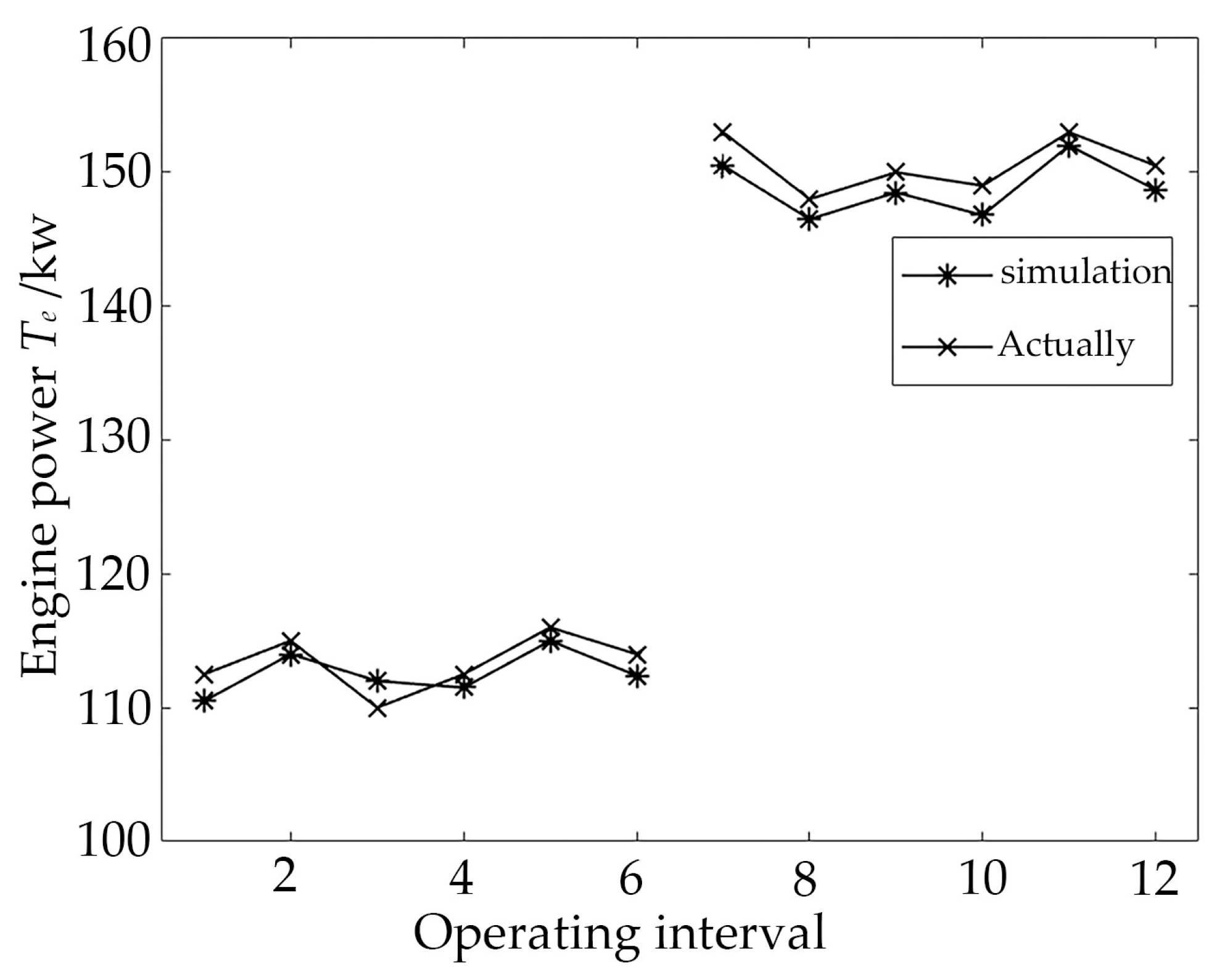
4.2. Model Validation Analysis of the Rotary-Tilling Tractor

Whether it is the study of rotary-tilling tractor fuel economy in this paper or the future study of variable speed control strategy of rotary-tiller operation, it is necessary to verify the reasonableness and accuracy of the power consumption model of the tractor unit. In this study, utilizing measured data from field rotary-tillage operation tests of the LW4004 high-power wheeled tractor, a power consumption simulation model for rotary-tillage operations was developed using the aforementioned backward dual-input modeling method to validate the accuracy and rationality of the unit transmission model.

The collected data included the PTO torque and the unit’s forward speed under two different forward speed conditions, each selected from a stable operation phase. The rotary tiller had a width of 4.5 m, an average tillage depth of approximately 0.2 m, an average PTO speed of 960 r/min, average forward speeds of 3.2 km/h and 4.9 km/h, and average PTO torques of 890 Nm and 1220 Nm. The green and blue data spectra in Figure 9 are the PTO torque loads during the stable operation phase at 3.2 km/h and 4.9 km/h operating conditions, respectively.

In Figure 9, during rotary-tiller operation, the PTO torque exhibited intense periodic fluctuations, which became more pronounced when the blades encountered hard objects. To minimize the impact of severe load fluctuations on the results and accurately depict the relationship between simulation results and measured data, the load spectra under the two operating speed conditions were segmented into six distinct time periods, with the average PTO torque and forward speed of the unit in each period used as input for the rotary tiller and traveling system simulation model, thereby verifying the accuracy and rationality of the unit drive simulation model.

After computing the load input using the simulation model, the horizontal thrust of the rotary tiller, the driving force of the tractor’s drive wheels, the transmission efficiency of the HMCVT, and the final coupling with engine power were determined. Under the experimental deep plowing conditions of the rotary tiller, the simulation results aligned more closely with the experimental data when the γ angle was set to 45°. Figure 10 presents a comparison between the simulated and measured results of the power consumption in the rotary-tiller group transmission system.

The simulation results in Figure 10 closely followed the trend of the measured values, demonstrating that the rotary-tillage driving system model, developed using the backward modeling method with dual load inputs, accurately represented the actual operating conditions of the unit. In the figure, when the unit advanced at high speed, the simulated engine power was slightly lower than the actual value. This discrepancy was likely due to factors in real-world operation, such as soil being thrown backward and striking the scraper plate, the scraper plate flattening the soil, the rotary tiller encountering side resistance, and the tractor experiencing wind resistance and other external interferences.

5. Fuel Consumption Model of Rotary-Tiller Group

5.1. Fuel Consumption per Unit of Operation for Rotary-Tillage Machinery

In tractor rotary-tillage operations, the amount of work completed per unit time, based on a certain quality standard, is referred to as unit productivity. Similarly, the fuel consumption incurred in completing a unit amount of work, under the same quality standard, is defined as unit fuel economy. Both factors are crucial considerations in the development of variable speed control strategies for rotary-tillage operation units.

The engine effective fuel consumption rate, g_e, is defined as the amount of fuel consumed by the engine per kilowatt-hour (kW·h) of work output. However, it only characterizes the fuel efficiency of the engine and does not reflect the fuel characteristics of the rotary-tilling tractor. In this paper, we introduced the concept ‘fuel consumption per kilometer of rotary-tillage operation, G_m’, to characterize the fuel efficiency of the rotary-tilling tractor.

Defined as the amount of fuel consumed by a tractor rotary-tiller unit, moving forward under uniform soil conditions and in accordance with a defined operating parameter, to complete one kilometer of tillage. Based on the unit’s operating parameters, machine power, and engine fuel characteristics, its expression can be derived as follows:

$$G_m={\displaystyle \frac{g_e{N}_e}{V_m}}$$

(14)

where G_m is the fuel consumption per kilometer of rotary operation, g/km; g_e is the engine effective fuel consumption rate, g/(kW·h); and V_m is the forward travel speed of the tractor, km/h.

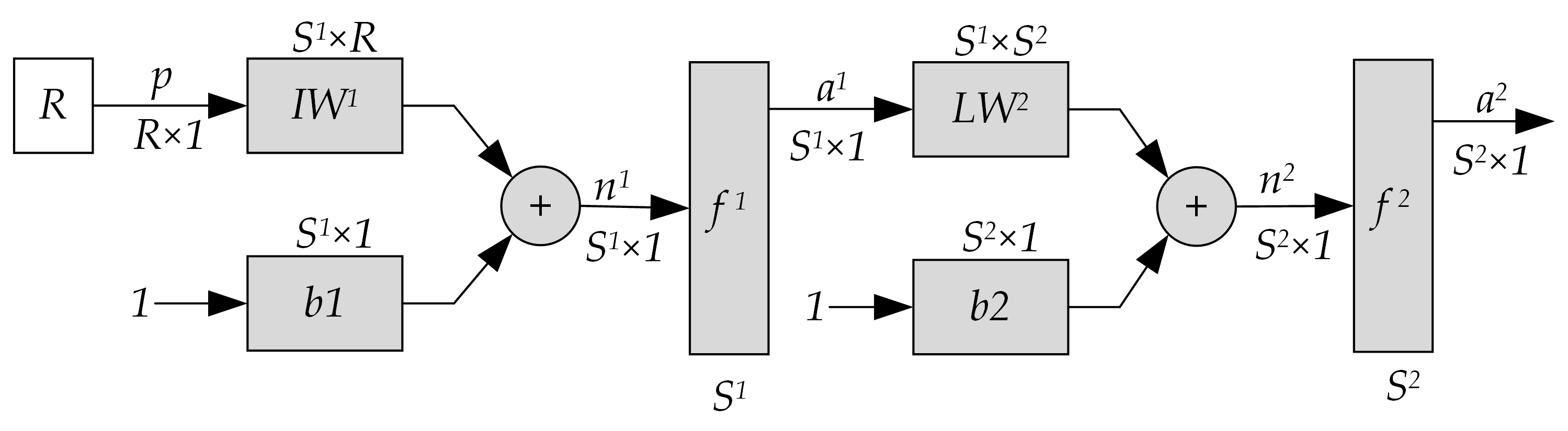
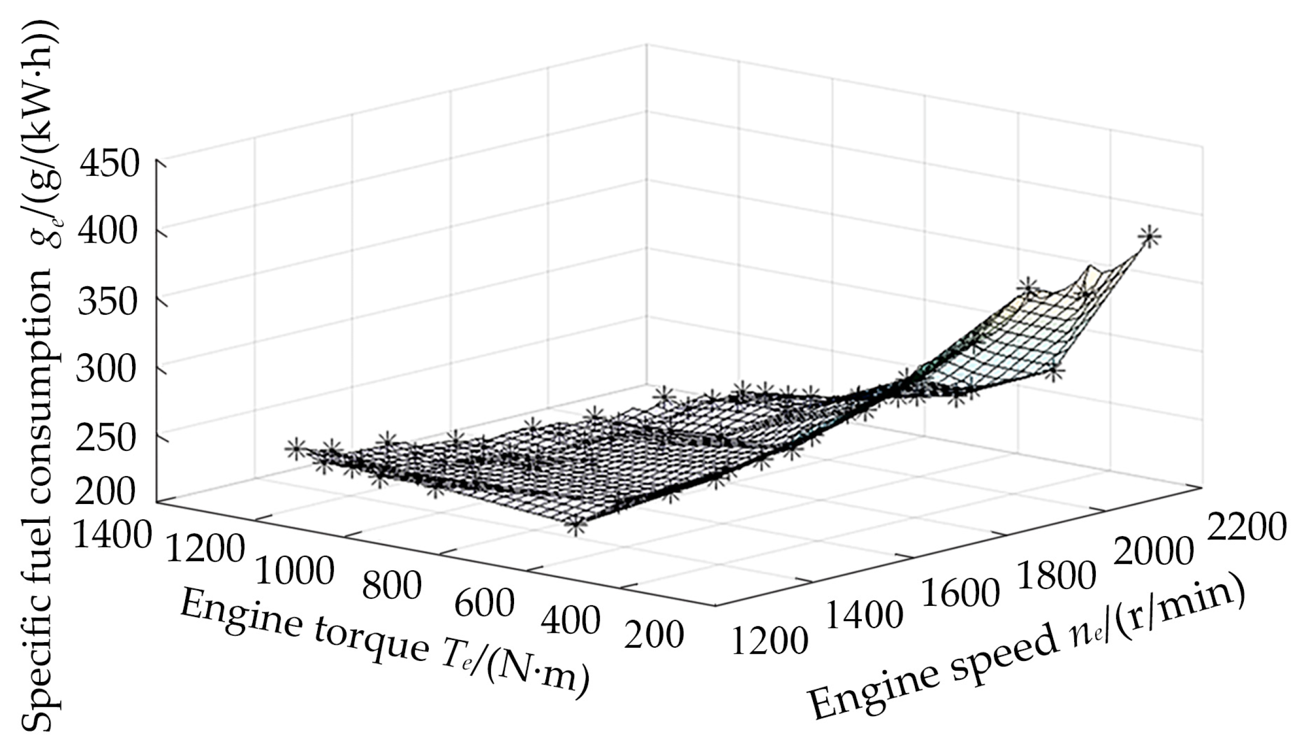
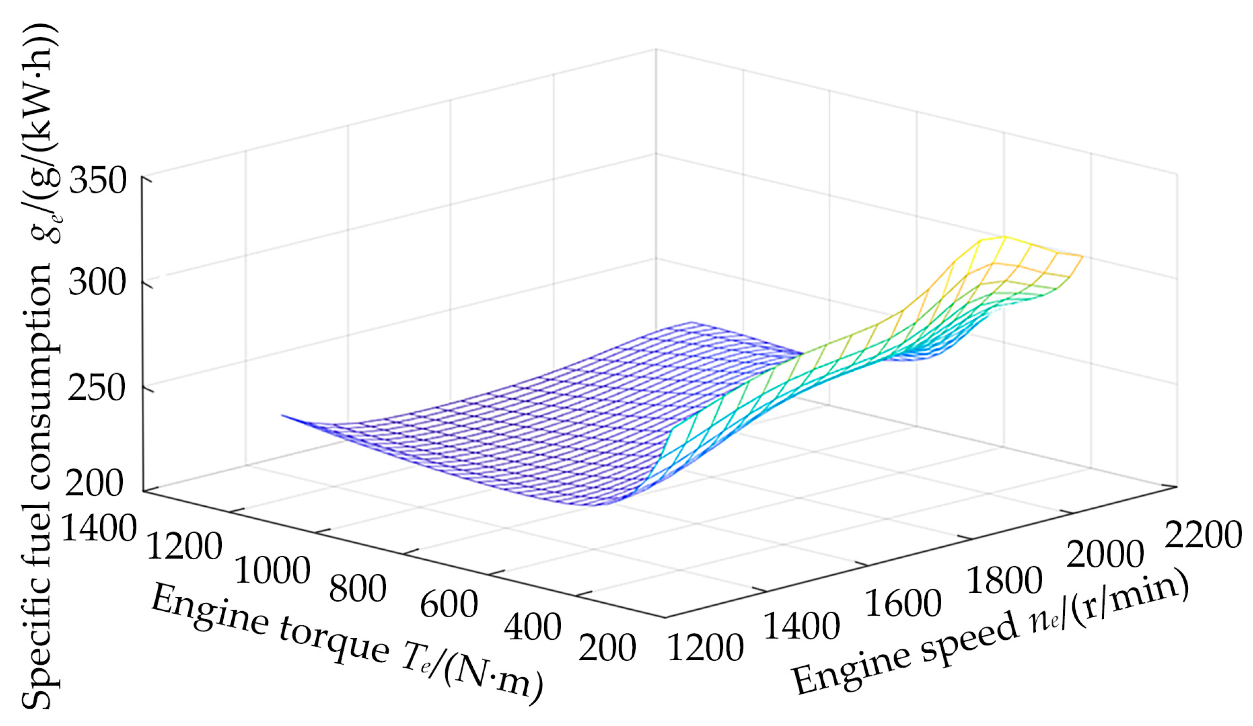
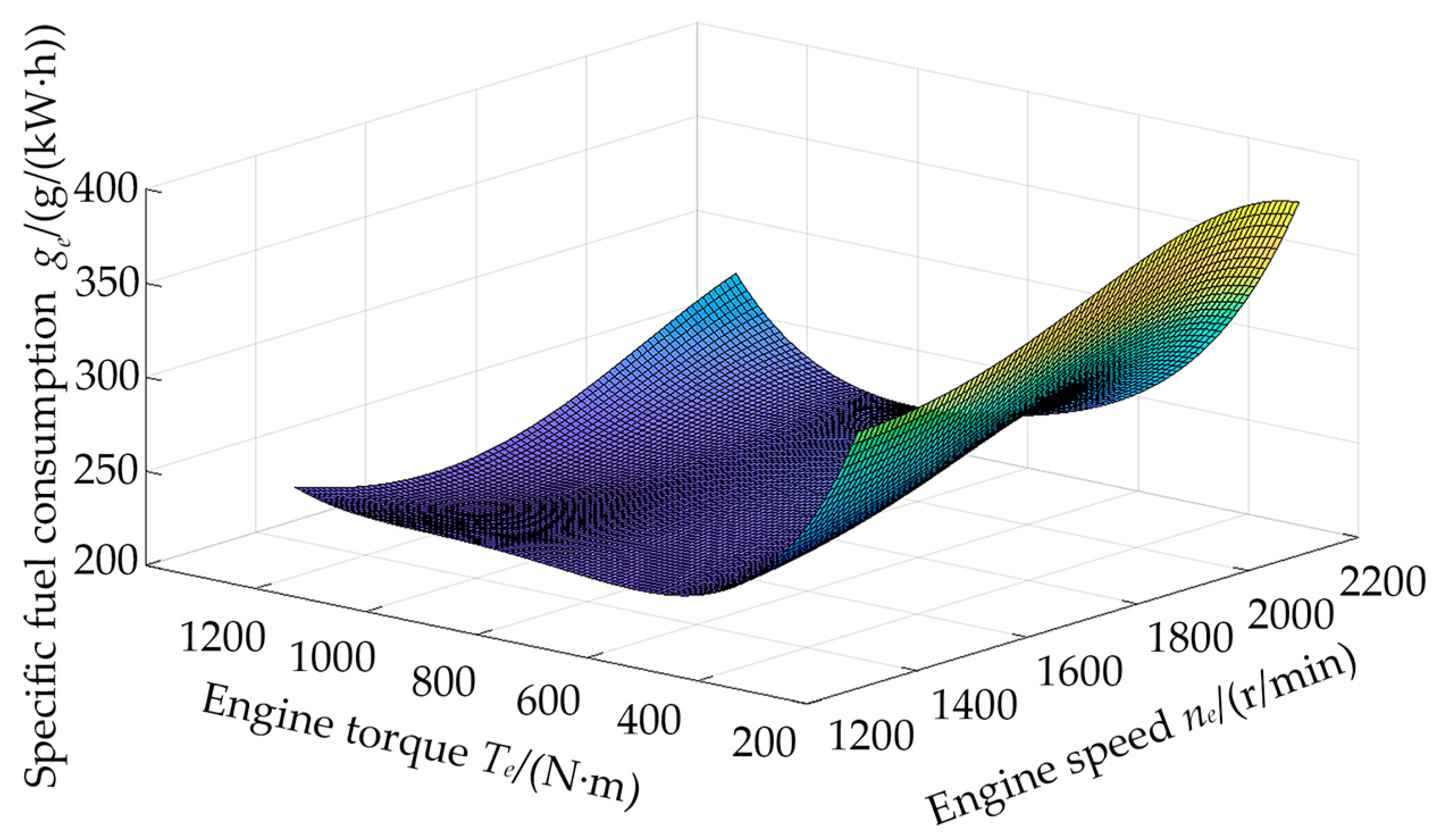
5.2. Mathematical Model of Diesel Engine Fuel Characteristics

An investigation into the fuel economy of a rotary-tilling tractor necessitates an accurate representation of the engine’s performance characteristics. Constructing a mathematical model of engine fuel characteristics essentially involves the quantitative expression and analysis of the nonlinear relationship between the variables of engine speed(n_e), torque (T_e), and engine effective fuel consumption rate (g_e).

Utilizing the excellent approximation ability of BP neural networks in dealing with complex nonlinear problems, the advantages of engine performance characteristics can be accurately captured by training only a certain amount of experimental data to construct a model of fuel characteristics close to reality. The BP neural network consists of multiple hidden layers, and increasing the number of hidden layers can reduce network error and enhance accuracy. However, this also increases the complexity of the network structure, extends training time, and can lead to network overfitting [25]. Scholars have theoretically proven that a single-hidden-layer BP network can perform any mapping from an n-dimensional to an m-dimensional space [26]. The topology of the single-hidden-layer BP neural network is illustrated in Figure 11.

In Figure 11, X_i is the network input; Y_i is the output; and ω_ij, ω_jk is the transfer function. It can be seen that the hidden layer includes multiple nodes, and the number of nodes is one of the key factors affecting the accuracy of the network.

A single-hidden-layer network was used to fit the characteristics of the diesel engine; the mathematical expression of this BP neural network is as follows:

$$a^2=f^2[L{W}^2{f}^1(I{W}^{1}p+b1)+b2]$$

(15)

In addition, the BP neural network model is shown in Figure 12.

In Figure 12, R denotes the dimension of the input vector; S₁ is the number of neurons in the hidden layer; S₂ is the number of output vectors; and p is the input vector. The variable a₁ is both the output of the hidden layer and the input vector of the output layer. The variable a₂ is the final output vector. IW₁, b₁, LW₂, and b₂ are the weights and thresholds of the hidden and output layers, respectively.

Based on the available 64 sets of test data for the ISLe310 engine in the LW4004 tractor, data were effectively divided into two subsets, a training set and a test set, in order to construct a single-hidden-layer BP neural network mathematical model for engine fuel characteristics.

To eliminate the difference in magnitude between the input and output data, and to enhance both the training efficiency and the generalization capability of the network, the mapminmax function was employed to normalize the input parameters, engine speed n_e, and torque T_e during computation. Inverse normalization was then applied to the model output, the effective fuel consumption rate (g_e):

$$y={\displaystyle \frac{(y_{\max }-y_{\min })(x-x_{\min })}{x_{\max }-x_{\min }}}-y_{\min }$$

(16)

In order to minimize the influence of the transfer function on the network error, it is necessary to make a reasonable selection of the transfer function of the implicit layer and the output layer.

The Log-sigmoid type transfer function was selected for the implicit layer. The output node was chosen to be a linear transfer function, purelin. The mathematical expression is as follows:

$$purelin(x)=x$$

(17)

$$\log sig(x)={\displaystyle \frac{1}{1+e^{-x}}}$$

(18)

When the number of hidden layer nodes in the model was set to 6, both the training error and test error reached their minimum values, and the function was represented by Equation (19).

$$g_e=purelin(L{W}_2\log sig(I{W}_1{\left[\begin{array}{l}{n}_e\\ T_e\end{array}\right]}_1+b_1)+b_2)$$

(19)

where engine speed n_e and torque T_e were the model input and the effective fuel consumption rate (g_e) were the model output. The weights and threshold coefficients are, respectively,

$$I{W}_1={\left[\begin{array}{c}6.4901\\ -2.7085\end{array}\begin{array}{c}8.2964\\ -10.0792\end{array}\begin{array}{c}4.2093\\ -8.4331\end{array}\begin{array}{c}-5.7945\\ 1.4938\end{array}\begin{array}{c}-3.6188\\ 3.0989\end{array}\begin{array}{c}0.0286\\ 8.4394\end{array}\right]}^T$$

$$L{W}_2=\left[-0.6395 0.6868 0.3051 0.5806 -0.2477 -4.9321\right]$$

$$b_1={\left[-6.4892 -11.3725 -2.7839 -7.9501 -0.2417 9.4010\right]}^T$$

$$b_2=\left[4.1876\right]$$

The distribution state of the engine fuel characteristic data points obtained from the experimental tests is shown in Figure 13, and the fuel consumption rate established using the BP neural network is shown in Figure 14.

Least squares is one of the most commonly used methods for data fitting, and the results of curve fitting the test data using least squares are shown in Figure 15.

The testing error of the engine fuel consumption characteristic model established by BP neural network was lower than 0.022, and the maximum testing error of the fitting result by the least squares method reached 0.07. Moreover, when using the least squares method to deal with the high load region, the fitting result was more different from the actual situation. By comparison, it can be learned that the engine fuel consumption characteristic model established by BP neural network can more accurately reflect the numerical relationship between fuel consumption rate (g_e), engine speed (n_e), and torque (T_e).

6. Results and Analysis of Results

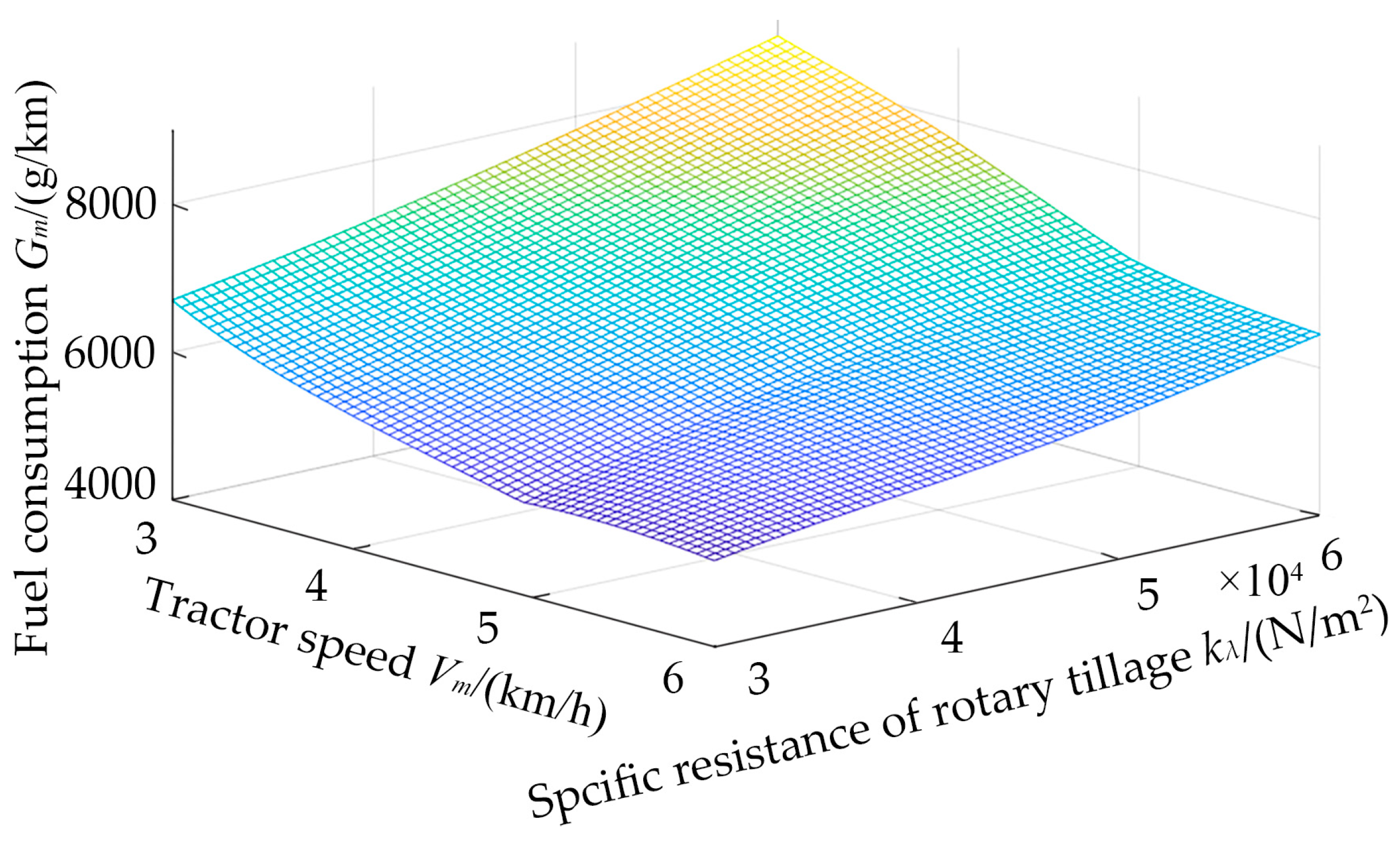
6.1. Fuel Consumption Characteristics of Rotary-Tilling Tractor

Under the operating conditions outlined in Section 3.1, the fuel consumption per kilometer of rotary-tillage operation model for the tractor is developed. Under the condition that the engine speed is always stabilized, continuously adjusting the HMCVT gear ratio, the fuel consumption characteristics of the tractor under different load conditions are shown in Figure 16.

Assuming uniform soil conditions within the same field, i.e., under a constant soil rotary-tillage resistance, it can be observed from Figure 13 that as the unit operating speed increases, the fuel consumption per kilometer of rotary-tillage operation (G_m) gradually decreases, while productivity improves.

However, as shown in Figure 15, when the forward speed of the tractor is less than 4.9 km/h, the rate of decrease in fuel consumption per kilometer of operation is significant with the increase in tractor speed. In contrast, when the forward speed exceeds 4.9 km/h, the decrease in fuel consumption per kilometer becomes less pronounced, and in regions where the soil rotary-tillage specific resistance is less than 35,000 N/m², the fuel consumption per kilometer of operation even increases.

6.2. Result Analysis

To investigate the causes of this phenomenon, the author examines the following three aspects:

(1) At a constant engine speed, increasing the HMCVT variable speed ratio to enhance the tractor’s forward speed results in an increase in the engine torque, leading to a decrease in the effective engine fuel consumption rate g_e, as shown in Figure 12, improving in engine efficiency. In other words, less fuel is consumed by the engine while delivering the same amount of power.

(2) As the unit’s forward speed increases, the torque on the rotary tiller’s knife shaft increases, which leads to a rise in the horizontal thrust exerted by the tiller on the tractor. It has been observed that without generating “parasitic power circulation,” the overall power utilization efficiency of the rotary-tilling tractor can be enhanced.

To examine the impact of load transfer on the overall power utilization efficiency of the rotary-tilling tractor, it is assumed that the power transmission efficiency of each system within the tractor, including the HMCVT, remains constant. For the purpose of expressing the power transmission efficiency of the unit, this paper defines the power utilization efficiency (ξ), which is the ratio of the useful work performed by the unit during operation, to the engine’s power:

$$\begin{array}{l}\xi ={\displaystyle \frac{N_{e1}}{N_{e0}}}={\displaystyle \frac{F_q{V}_m+N_r}{\frac{F_q{V}_m}{{\eta }_q}+\frac{N_r}{{\eta }_r}}}\\ F_q=(\mu (M+m)g-F_x)\end{array}$$

(20)

In the load characteristic field, the variation of power utilization efficiency ξ is shown in Figure 17.

As the forward speed V_m of the tractor increases and the k_λ of the rotary-tiller resistance rises, the horizontal thrust F_x exerted by the rotary tiller on the tractor increases, making the load transfer phenomenon more apparent. As shown in Figure 16, it leads to a corresponding increase in ξ, indicating a continuous improvement in the unit’s power utilization efficiency.

(3) Based on the required traveling speed of the tractor during rotary-tillage operation, it is observed that the multi-segment HMCVT predominantly operates in the first hydro-mechanical segment, with its segment transmission efficiency varying in accordance with the variable speed ratio under no load transfer conditions, as shown in Figure 18.

As the variable speed ratio increases, with the efficiency of the HMCVT initially rising and then declining, the highest efficiency is achieved when the HMCVT operates in its purely mechanical mode. To investigate the impact of HMCVT efficiency variation on tractor fuel consumption, this study specifically establishes extreme working conditions characterized by the highest soil rolling resistance coefficient and the lowest rotary-tillage specific resistance. The rotational tillage specific resistance is set within the range of 30–35 kN/m². Under such conditions, the power demand for the tractor’s traveling mechanism becomes substantially elevated, where efficiency fluctuations in the HMCVT system exert significant influence on engine load regulation.

As the tractor’s traveling speed continues to increase, after the transmission ratio of the HMCVT system passes the peak efficiency point, its transmission efficiency decreases. This phenomenon results in a marginal increase in fuel consumption per unit operation within the specific resistance range of 30–35 kN/m². However, such extreme operating conditions rarely occur in practice. In other operational ranges, where soil specific resistance is relatively high, increasing the tractor’s speed further amplifies the thrust force exerted by the rotary tiller onto the tractor. This reduction in required driving force for the wheels subsequently diminishes the impact of HMCVT efficiency variations on engine load. Consequently, the fuel consumption characteristic for unit work volume continues exhibiting a downward trend.

This observation aligns with the conclusion stated in the paper: An increase in tractor forward speed simultaneously enhances the productivity and fuel economy of the rotary-tiller unit. However, higher speeds lead to a reduction in the rotary-tiller speed ratio (λ), which compromises the quality of tillage operations. Therefore, the forward speed of the unit must be restricted within a reasonable range. These findings thereby establish a theoretical foundation for subsequent research on variable speed control strategies that balance the comprehensive performance of tractor rotary-tillage operations.

7. Conclusions

(1)

When the rotary-tilling tractor operates in a soft soil environment, changes in the efficiency of the HMCVT at different speed ratios have a more pronounced impact on both the power characteristics and fuel consumption behavior of the machine. This factor must be carefully considered when developing an accurate dynamic model of the system.

(2)

Focusing on the characteristics of the rotary-tilling tractor and considering the dynamic interaction between the rotary tiller, the tractor drive wheels, and the transmission efficiency of the multi-segment HMCVT, the unit dynamic model established using the backward dual-input modeling method accurately captures the relationship between the unit’s travel system, rotary-tillage loads, and engine power consumption. In the analysis of unit productivity, the maximum engine load rate emerges as the most critical factor limiting productivity.

(3)

By introducing the fuel consumption per kilometer of rotary-tillage operation G_m to characterize the fuel consumption characteristics of the rotary-tillage unit, the research findings indicate that increasing the unit’s forward speed leads to a reduction in fuel consumption per kilometer of rotary operation G_m. Therefore, provided a certain work quality is maintained, enhancing the forward speed of the unit simultaneously improves both work efficiency and fuel economy. This provides a theoretical foundation for future research on the variable speed control strategy of rotary-tilling tractors.

References

1. Mocera, F.; Soma, A.; Martelli, S.; Martini, V. Trends and Future Perspective of Electrification in Agricultural Tractor-Implement Applications. Energies 2023, 16, 6601. [Google Scholar] [CrossRef]
2. Xiao, M.; Niu, Y.; Wang, K.; Zhu, Y.; Zhou, J.; Ma, R. Design of Self-Excited Vibrating Its Performance in Reducing Rotary Tiller and Analysis of Torsion and Consumption. Trans. Chin. Soc. Agric. Mach. 2022, 53, 52–63. [Google Scholar]
3. Zhang, J.; Feng, G.; Yan, X.; He, Y.; Liu, M.; Xu, L. Cooperative Control Method Considering Efficiency and Tracking Performance for Unmanned Hybrid Tractor Based on Rotary Tillage Prediction. Energy 2024, 288, 129874. [Google Scholar] [CrossRef]
4. Yang, H.; Zhou, J.; Qi, Z.; Sun, C.; Lai, G. Research on Rotary Tillage Stability of Greenhouse Electric Tractor Based on Time Series Analysis and Feedforward PID. Trans. Chin. Soc. Agric. Mach. 2024, 55, 412–420. [Google Scholar]
5. Kozhushko, A.; Pelypenko, Y.; Mittsel, M.; Veretennikov, I.; Kalnaguz, A.; Trembach, O.; Stanciu, A. Analysing the Response of a Dual-Flow Transmission (HMCVT) for Wheeled Tractors According to Efficiency and Productivity Criteria. Int. J. Mechatron. Appl. Mech. 2024, 16, 33–41. [Google Scholar]
6. Zhang, Z.; Li, X.; Peng, Z.; Jing, C.; Yang, S.; Chen, Z. Full-condition efficiency model and power loss analysis of hydro-mechanical CVT. Trans. Chin. Soc. Agric. Eng. 2024, 40, 48–58. [Google Scholar]
7. Liang, L.; Li, Q.; Tan, Y.; Yang, Z. Multi-parameter Optimization of HMCVT Fuel Economy Using Parameter Cyclic Algorithm. Trans. Chin. Soc. Agric. Eng. 2023, 39, 48–55. [Google Scholar]
8. Huang, X.; Lu, Z.; Chen, L.; Qian, J.; An, Y. Optimization of Tractor HMCVT Target Speed Ratio and Control Simulation Based on Machine Economy. J. Nanjing Agric. Univ. 2022, 45, 777–787. [Google Scholar]
9. Ahn, S.; Choi, J.; Kim, S.; Lee, J.; Choi, C.; Kim, H. Development of an Integrated Engine-Hydro-Mechanical Transmission Control Algorithm for a Tractor. Adv. Mech. Eng. 2015, 7, 1–18. [Google Scholar] [CrossRef]
10. Cao, F.; Li, W.; Han, Q.; Zhang, M. Switching of the Comprehensive Mode for the Hydro-Mechanical Continuously Variable Transmission of a Tractor. Trans. Chin. Soc. Agric. Eng. 2022, 38, 41–47. [Google Scholar]
11. Zhang, J.; Feng, G.; Liu, M.; Yan, X.; Xu, L.; Shang, C. Research on Global Optimal Energy Management Strategy of Agricultural Hybrid Tractor Equipped with CVT. World Electr. Veh. J. 2023, 14, 127. [Google Scholar] [CrossRef]
12. Li, B.; Sun, D.; Hu, M.; Liu, J. Research on Economic Comprehensive Control Strategies of Tractor-Planter Combinations in Planting, Including Gear-Shift and Cruise Control. Energies 2018, 11, 686. [Google Scholar] [CrossRef]
13. Hu, J.; Zhao, J.; Pan, H.; Liu, W.; Zhao, X. Prediction Model of Double Axis Rotary Power Consumption Based on Discrete Element Method. Trans. Chin. Soc. Agric. Mach. 2020, 51, 9–16. [Google Scholar]
14. Mirzaev, B.; Steward, B.; Mamatov, F.; Tekeste, M.; Amonov, M. Analytical Modeling Soil Reaction Forces on Rotary Tiller. In Proceedings of the An ASABE Meeting Presentation, St. Joseph, MI, USA, 12–16 July 2021. [Google Scholar]
15. Xiong, P.; Yang, Z.; Sun, Z.; Zhang, Q.; Huang, Y.; Zhang, Z. Simulation Analysis and Experiment for Three-axis Working Resistances of Rotary Blade Based on Discrete Element Method. Trans. Chin. Soc. Agric. Eng. 2018, 34, 113–121. [Google Scholar]
16. Patidar, P.; Soni, P.; Jain, A.; Mahore, V. Modelling soil-rotor blade interaction of vertical axis rotary tiller using discrete element method (DEM). J. Terramechanics 2024, 112, 59–68. [Google Scholar] [CrossRef]
17. Wang, Z.; Huang, Y.; Li, Z.; Jia, H.; Wan, B. Universal the Blade the Broken Stubble Power Consumption Influence of the Working Parameters of the Rotary Tiller Broken Stubble. J. Jilin Univ. (Eng. Technol. Ed.) 2012, 42, 122–125. [Google Scholar]
18. Zhao, H.; Li, Y.; Zeng, Q.; Liu, D. Simulation of Rotary Tiller Based on MATLAB. Journal of Northwest A F Univ. (Nat. Sci. Ed.) 2016, 44, 230–234. [Google Scholar]
19. Fang, H.; Ji, C.; Zhang, Q.; Gou, J. Force Analysis of Rotary Blade Based on Distinct Element Method. Trans. Chin. Soc. Agric. Eng. 2016, 32, 54–59. [Google Scholar]
20. Luoyang Tractor Research Institute; Ministry of Mechanical and Electronics Industry. Tractor Design Manual, 2nd ed.; China Machine Press: Beijing, China, 1994; pp. 209–216. [Google Scholar]
21. Zhao, J.; Liu, M.; Xu, L.; Yu, S.; Xie, P. Prediction Model and Experiment on Tractive Performance of Four-wheel Drive Tractor. Trans. Chin. Soc. Agric. Mach. 2023, 54, 439–447. [Google Scholar]
22. Zhang, M.; Wang, J.; Wang, J.; Guo, Z.; Guo, F.; Xi, Z.; Xu, J. Speed Changing Control Strategy for Improving Tractor Fuel Economy. Trans. Chin. Soc. Agric. Eng. 2020, 36, 82–89. [Google Scholar]
23. Li, H.; Song, Z.; Xie, B. Plowing Performance Simulation and Analysis for Hybrid Electric Tractor. Appl. Mech. Mater. 2013, 365–366, 505–511. [Google Scholar] [CrossRef]
24. Lee, H.; Kim, J.; Park, Y.; Cha, S. Rule-Based Power Distribution in the Power Train of a Parallel Hybrid Tractor for Fuel Savings. Int. J. Precis. Eng. Manuf.-Green Technol. 2016, 3, 231–237. [Google Scholar] [CrossRef]
25. Li, Q.; Jia, W. Phase Selection and Location Method of Generator Stator Winding Ground Fault Based on BP Neural Network. Energies 2023, 16, 1503. [Google Scholar] [CrossRef]
26. Lu, Q.; Su, K.; Zhang, J.; Yan, T.; Yang, B.; Zhang, H. Structural Optimization of Simple Catenary Based on BP Neural Network and Genetic Algorithm. J. Mech. Eng. 2024, 60, 313–320. [Google Scholar]
Figure 1. Force diagram of rotary-tilling tractor.
Energies 18 01490 g001
Figure 2. Diagram of transmission system of rotary-tilling tractor.
Energies 18 01490 g002
Figure 3. The torque coupling diagram of the rotary-tilling tractor.
Energies 18 01490 g003
Figure 4. The power flow analysis for three operating states.
Energies 18 01490 g004
Figure 5. Force analysis of single-blade soil cutting operation of rotary tiller.
Energies 18 01490 g005
Figure 6. Schematic diagram of multi-range hydro-mechanical CVT.
Energies 18 01490 g006
Figure 7. Schematic diagram of backward modeling of rotary-tilling tractor.
Energies 18 01490 g007
Figure 8. Load characteristics of rotary-tilling tractor. The colors in the graph go from blue to yellow and represent only the change in the magnitude of the z-axis variable values.
Energies 18 01490 g008
Figure 9. PTO torque load at some moments in the stable operation stage. The green and blue colors in the figure represent the load spectrum of PTO torque at 3.2 km/h and 4.9 km/h, respectively.
Energies 18 01490 g009
Figure 10. Model simulation results.
Energies 18 01490 g010
Figure 11. Single-hidden-layer BP neural network topology. In the figure, green represents the input layer; blue represents the hidden layer; and yellow represents the output layer. Figure 11 contains an explanation of them.
Energies 18 01490 g011
Figure 12. The network model of the BP neural network.
Energies 18 01490 g012
Figure 13. Fuel characteristic test data point distribution map.
Energies 18 01490 g013
Figure 14. Diesel engine fuel consumption characteristics. The colors in the graph go from blue to yellow and represent only the change in the magnitude of the z-axis variable values.
Energies 18 01490 g014
Figure 15. Results of least squares fitting. The colors in the graph go from blue to yellow and represent only the change in the magnitude of the z-axis variable values.
Energies 18 01490 g015
Figure 16. Fuel consumption per unit operation of rotary-tilling tractor. The colors in the graph go from blue to yellow and represent only the change in the magnitude of the z-axis variable values.
Energies 18 01490 g016
Figure 17. The power utilization efficiency of the rotary-tilling tractor. The colors in the graph go from blue to yellow and represent only the change in the magnitude of the z-axis variable values.
Energies 18 01490 g017
Figure 18. Transmission efficiency variations of the hydro-mechanical CVT.
Energies 18 01490 g018