Multi-Factor Carbon Emissions Prediction in Coal-Fired Power Plants: A Machine Learning Approach for Carbon Footprint Management

Abstract

In coal-fired power plants, accurately accounting for carbon footprints is crucial for reducing greenhouse gas emissions and achieving sustainability goals. Life cycle assessment (LCA) is a comprehensive approach that expands the scope of carbon accounting, enabling the calculation of carbon emission data. However, the unclear boundary definition and incomplete data types often lead to insufficient accuracy in model calculations and predictive performance. Herein, we developed machine learning models to predict carbon emissions in a 1000 MW coal-fired power plant. The ElasticNet modeling approach demonstrated exceptional predictive accuracy (R² = 0.9514; MAE = 435.42 metric tons CO₂). Coal combustion constituted the predominant source of greenhouse gas emissions, with quarterly emissions reaching 1.63 million metric tons in Q1 and 1.11 million metric tons in Q3. Emission intensity exhibited remarkable stability across operational load ranges (1.0–1.1 kg/MWh). Notably, under high-load conditions (>70%), low-calorific-value coal generated marginally higher specific emissions (1.11 kg/MWh) compared to high-calorific-value coal (1.05 kg/MWh). The findings provide rational strategies for optimizing coal procurement strategies and environmental control measures, thereby facilitating an optimal balance between operational efficiency and environmental stewardship.

1. Introduction

Pervasive carbon dioxide (CO₂) emissions exacerbate global warming and environmental issues. In China, carbon emissions from energy activities account for approximately 88% of total CO₂ emissions, with the power industry contributing around 42% of the energy sector’s carbon emissions, primarily from coal-fired power generation. To achieve the goals of carbon peaking and carbon neutrality, the energy sector is the main battlefield, the power industry is the main force, and coal-fired power generation is the breakthrough point [1,2,3,4,5,6].

Carbon accounting is the primary foundation for carrying out de-carbon work. Currently, the internationally recognized carbon accounting methods for coal-fired power plants include the emission factor method, material balance method, direct measurement method, model method, and life cycle assessment (LCA) [7,8,9,10,11]. Among these, the emission factor method has the widest application scope and a simple calculation process. However, directly using the default emission factor values from the IPCC guidelines to calculate the carbon emissions of China’s coal-fired power plants results in significant errors. The material balance method utilizes carbon balance to calculate the carbon emissions of coal-fired power plants, but the calculation process involves many intermediate steps and requires complete data to obtain accurate carbon emission values. The direct measurement method can directly measure the flue gas flow rate and CO₂ concentration in the flue gas, but few coal-fired power plants in China have complete continuous emission monitoring systems (CEMS) [12,13,14,15]. The model method can directly predict carbon emissions or elemental carbon content, addressing the issue of missing key accounting data, but there are significant deviations between the mathematical models and actual values. Compared to the above methods, LCA can expand the scope of accounting, both upstream and downstream, enabling the more accurate calculation of carbon emission data [14].

As global efforts toward carbon peak and neutrality intensify, coal-fired power plants are undergoing dual transformational shifts [16,17,18]. First, these facilities are evolving to serve both as baseline power guarantors and grid regulators, resulting in widely fluctuating operational conditions that directly impact CO₂ emission intensities [19]. Second, to meet carbon neutrality requirements, these plants are accelerating the development and systematic integration of novel clean energy technologies, leading to substantial reductions in carbon emissions [20]. In this dynamic context, conventional methods including emission factor calculations, material balance approaches, direct measurements, and modeling prove inadequate in accurately characterizing the complex carbon emission profiles of coal-fired facilities. These methods fail to effectively classify and weight the multidimensional operational parameters inherent in these plants.

As global climate change issues become increasingly prominent, research on carbon emission factors and reduction strategies continues to deepen. Du et al. evaluated the impact of financial policies on carbon emission efficiency in Chinese cities from a green finance policy perspective, using China’s green finance reform and innovation pilot zones (GFRIP) as a natural experiment with a difference-in-differences (DID) approach. The research demonstrates that green finance reforms significantly improved carbon emission efficiency through promoting green innovation, expanding financial supply, optimizing industrial structure, and enhancing energy efficiency [21]. This macroeconomic policy perspective provides important insights for understanding the institutional environment of energy structure transformation, offering a broader policy background for our micro-level carbon emission prediction research.

Recent advancements in machine learning approaches have significantly enhanced carbon emission accounting methodologies in the energy sector. Liu et al. developed an LSTM-Attention model for regional power system carbon emission measurement, demonstrating improved accuracy over traditional accounting methods by capturing temporal dependencies in emission patterns [10]. Similarly, Mariutti applied machine learning techniques to analyze the carbon footprint of photovoltaic modules manufactured in China, revealing significant variations in emissions that conventional methods failed to detect [11]. These studies highlight the growing importance of advanced algorithmic approaches in enhancing the precision of carbon accounting beyond traditional LCA frameworks.

Recent studies have expanded our understanding of carbon footprint reduction strategies across various technologies. Cobos-Torres et al. investigated the potential of renewable energies and biochar as green alternatives for reducing carbon footprints using tree species from the Andean region of Ecuador, demonstrating significant emission reduction potential through integrated approaches [6]. These findings complement our investigation by highlighting the importance of considering alternative energy sources alongside the optimization of existing coal-fired technologies.

Studies propose a rational approach combining LCA with machine learning algorithms to address these limitations [22,23,24,25,26]. This methodology expands the accounting boundary to comprehensively capture emission variations resulting from deep peak regulation and clean energy technology integration [27,28]. The framework enables real-time predictions using large-scale, multidimensional daily operational data while identifying key factors influencing carbon emissions in coal-fired facilities. This integration offers precise carbon calculations across the entire life cycle of coal power projects, facilitating the establishment of standardized carbon emission accounting systems.

Herein, a comprehensive analytical framework was studied that integrates LCA with machine learning algorithms to process extensive operational parameters from coal-fired power facilities. We seek to develop and evaluate multiple machine learning models for carbon emissions prediction in coal-fired power generation facilities and identify the most significant factors influencing carbon emissions through feature importance analysis. Then, we compare the performance of different algorithms in terms of accuracy, computational efficiency, and interpretability and provide practical recommendations for implementing machine learning-based emissions monitoring systems in coal-fired power plants. These findings provide the potential of interpretable machine learning models for environmental management in coal-fired facilities. The novelty of this work lies in the unprecedented integration of feature importance analysis with temporal modeling, revealing, for the first time, the complex interplay between coal quality parameters and seasonal factors in determining carbon emission patterns. Unlike previous studies that examined these factors in isolation, our approach provides a comprehensive understanding of their combined effects, offering a more nuanced framework for emissions management in coal-fired facilities.

2. Materials and Methods

2.1. Calculation Model for Coal-Fired Power Plants

Based on our dataset characteristics and research objectives, we have constructed the emissions calculation model. The following aspects of emissions are mainly considered:

2.1.1. Coal Combustion Emissions

Coal combustion is the main source of CO₂ emissions [29,30,31,32], and the related parameters were calculated as follows:

$$E_{\mathrm{combustion}}=\sum _{i=1}^2\left(W_{\mathrm{coal},i}\times {\displaystyle \frac{C_{\mathrm{volatile}}}{100}}\times {\displaystyle \frac{M_{{\mathrm{CO}}_2}}{M_c}}\times O{F}_i\right)$$

(1)

where $W_{\mathrm{coal},i}$ is the coal consumption of unit i (coal_consumption_1/2), $C_{\mathrm{volatile}}$ is the volatile content of coal (volatile), $M_{{\mathrm{CO}}_2}/M_c$ is the molecular mass ratio of CO₂ to C (44/12), and $O{F}_i$ is the oxidation factor of unit i (estimated through PEC_1/2).

The oxidation factor (OF) values were estimated based on empirical plant operational data and validated against the IPCC default value. This empirical derivation ensures that the carbon conversion calculations reflect the specific combustion efficiency characteristics of the studied facility, rather than relying solely on the generalized literature values.

2.1.2. Desulfurization Process Emissions

CO₂ emissions from the desulfurization process are calculated as

$$E_{\mathrm{desulf}}=W_{\mathrm{gypsum}}\times {\gamma }_{{\mathrm{CaCO}}_3}\times {\displaystyle \frac{M_{{\mathrm{CO}}_2}}{M_{{\mathrm{CaCO}}_3}}}$$

(2)

where $W_{\mathrm{gypsum}}$ is the gypsum production (gypsum), ${\gamma }_{{\mathrm{CaCO}}_3}$ is the calcium carbonate conversion coefficient, and $M_{{\mathrm{CO}}_2}/M_{{\mathrm{CaCO}}_3}$ is the molecular mass ratio (44/100).

2.1.3. Ash-Handling Emissions

CO₂ emissions from the ash-handling process are calculated as

$$E_{\mathrm{ash}}=\left(W_{\mathrm{raw}\_\mathrm{ash}}+W_{\mathrm{wet}\_\mathrm{ash}}+W_{\mathrm{furnace}\_\mathrm{slag}}\right)\times {\eta }_{\mathrm{ash}}$$

(3)

where $W_{\mathrm{raw}\_\mathrm{ash}}$ is the dry ash amount (raw_ash), $W_{\mathrm{wet}\_\mathrm{ash}}$ is the wet ash amount (wet_ash), $W_{\mathrm{furnace}\_\mathrm{slag}}$ is the furnace slag amount (furnace_slag), and ${\eta }_{\mathrm{ash}}$ is the emission factor for ash handling.

2.1.4. Comprehensive Efficiency Correction

Considering the impact of unit load and efficiency:

$${\eta }_{\mathrm{total},i}={\displaystyle \frac{{\mathrm{PEC}}_i}{{\mathrm{load}}_i}}\times {\beta }_{\mathrm{moisture}}\times {\beta }_{\mathrm{heat}}$$

(4)

where ${\mathrm{PEC}}_i$ is the plant electricity consumption rate (PEC_1/2), ${\mathrm{load}}_i$ is the unit load (load_1/2), ${\beta }_{\mathrm{moisture}}$ is the moisture correction factor, related to coal_moisture, and ${\beta }_{\mathrm{heat}}$ is the heat value correction factor, related to heat_value_received.

2.1.5. Total Emissions Calculation

The final CO₂ total emissions calculation formula:

$$E_{\mathrm{total}}=\left(E_{\mathrm{combustion}}\times {\eta }_{\mathrm{total}}\right)+E_{\mathrm{desulf}}+E_{\mathrm{ash}}$$

(5)

Note that all calculations consider the time-series characteristics of the data, the calculations consider changes in the coal quality parameters (moisture, volatile matter, heat value, etc.), dynamic changes in unit efficiency and load are considered, and emissions from desulfurization and ash handling are calculated as secondary emission sources.

2.2. Data Collection

The dataset for this study was collected from a 1000 MW coal-fired power plant during the year 2023. It includes daily measurements of operational parameters and resource consumption metrics, critical for understanding carbon emissions dynamics. Key variables in the dataset encompass the following: coal characteristics such as moisture content, volatile matter, and calorific value; operational data including coal consumption and power load for both generating units (Unit 1 and Unit 2); plant electricity consumption (PEC) for each unit; by-products such as gypsum, ash (raw and wet), and furnace slag production. Additionally, total water consumption and solar power generation (SPG) data from four sections (A, B, C, and D) are included, reflecting the plant’s contribution to renewable energy generation. These data, collected daily from both units, provide comprehensive guidance into plant performance and emissions profiles.

2.3. Data Preprocessing

The raw data underwent several preprocessing steps to ensure quality and reliability. Missing values were identified and handled using appropriate statistical methods, including interpolation techniques for temporal data gaps and the removal of records with excessive missing values. Outlier detection employed statistical methods to identify extreme values, which were then validated against operational records. Robust scaling was applied to handle outliers while preserving important variations. Feature engineering involved creating derived features by combining related parameters, normalizing continuous variables, and encoding categorical variables where applicable.

Feature engineering played a crucial role in enhancing model performance. We developed several interaction features capturing the combined effects of related parameters. Most notably, the ‘load × calorific value’ interaction feature demonstrated a strong correlation with emissions (r = 0.76), exceeding the predictive power of either load (r = 0.65) or calorific value (r = 0.58) individually. This interaction term effectively captured the varying energy conversion efficiency of coal under different load conditions, providing deeper insights into plant performance dynamics.

Temporal feature engineering included the creation of seasonal indicators through sinusoidal transformations of date components (sin/cos transformations) and a monthly load index that captured seasonal electricity demand patterns. These derived features exhibited a moderate correlation with emissions (r = 0.42), enabling the model to account for cyclical variations in plant operations and environmental conditions that influence emission patterns throughout the year.

Missing values, which constituted less than 5% of the total dataset, were handled using specific techniques based on data type. For time-series parameters, forward filling was employed to maintain temporal continuity, while K-nearest neighbor imputation (k = 3) was used for non-sequential missing data points. This approach preserved the temporal structure of the dataset while minimizing imputation errors.

Outlier detection employed a 3σ rule to identify potential anomalies, which were then cross-validated against operational records to distinguish between measurement errors and genuine operational fluctuations. Confirmed outliers were treated using a Winsorization approach (at the 95th percentile) to reduce their influence without complete removal, thereby preserving valuable information about extreme operating conditions while mitigating their disproportionate impact on model training.

2.4. Exploratory Data Analysis

An initial analysis of the dataset revealed several important characteristics. Temporal patterns showed significant seasonal variations in coal consumption and power generation, daily and weekly patterns in operational parameters, and correlations between environmental conditions and efficiency metrics. Variable relationships indicated strong correlations between coal quality parameters and emissions, non-linear relationships between operational parameters, and interdependencies between environmental factors and plant performance. Data quality assessment showed a high completeness rate (>95%) for critical parameters, consistent measurement frequencies, and reliable sensor calibration and maintenance records.

2.5. Model Development and Evaluation

This study employs multiple machine learning algorithms to predict carbon emissions, including linear regression, ridge regression, lasso regression, and ElasticNet. These models were chosen to capture different aspects of the data relationships, from simple linear correlations to complex regularized models. The model training process involved splitting the data into 70% training and 30% testing sets, using 5-fold cross-validation for robust evaluation, and employing grid search for optimal hyperparameter selection. Feature engineering incorporated polynomial features, interaction terms, and time-based features to capture non-linear relationships and seasonal patterns.

Our methodological approach builds upon recent advancements in emissions modeling techniques. Liu et al. proposed an LSTM-Attention model for carbon emission measurement in regional power systems [10], achieving impressive accuracy through deep learning architectures. While our approach differs in favoring interpretable linear models, we adopt similar principles of feature importance analysis and temporal pattern recognition. The trade-off between complex black-box models with marginally higher accuracy and more interpretable models with actionable insights represents a fundamental consideration in emissions modeling that warrants careful evaluation based on specific application requirements.

The data split methodology strictly adhered to chronological order, using the first 9 months (January–September) for training and the final 3 months (October–December) for testing. This temporal separation ensures that future data points never inform predictions of earlier periods, preventing data leakage that could artificially inflate model performance metrics. Additionally, to assess model stability over time, we implemented a 3-month rolling window validation approach, using each 3-month period to predict the subsequent month and then rolling forward. The model demonstrated remarkable temporal stability across these windows, with an R² standard deviation of only 0.023, confirming its reliability across different seasonal and operational conditions throughout the year.

Each model underwent extensive hyperparameter tuning. For ridge regression, alpha values of 0.1, 1.0, and 10.0 were tested with ‘lsqr’ and ‘sag’ solver options. Lasso regression used the same alpha values with ‘cyclic’ and ‘random’ selection methods. ElasticNet optimization included alpha values of 0.1, 1.0, and 10.0, L1 ratios of 0.1, 0.5, and 0.9, and both ‘cyclic’ and ‘random’ selection methods.

The models were evaluated using multiple metrics to ensure comprehensive performance assessment. Primary metrics included the Mean Absolute Error (MAE), R² score, and Explained Variance Score. Additional analyses involved residual analysis, feature importance ranking, model stability assessment through cross-validation, and prediction interval estimation. The validation strategy incorporated time-based validation, out-of-sample testing on unseen data, and a sensitivity analysis for key parameters.

The implementation utilized Python 3.8 with Scikit-learn for model implementation, Pandas for data manipulation, and NumPy for numerical computations. The model pipeline included standardization of the features, missing value imputation, feature selection, and model training and evaluation.

While deep learning models such as Long Short-Term Memory (LSTM) networks have demonstrated exceptional performance in time-series forecasting applications, they were not prioritized in this study for several reasons. First, the relatively limited dataset size (365 daily records) is insufficient to fully leverage the capabilities of complex neural architectures, potentially leading to overfitting issues. Second, the “black-box” nature of deep learning models significantly reduces interpretability, which conflicts with our primary objective of understanding parameter influence mechanisms on emissions. The regularized linear models selected for this study balance predictive accuracy with interpretability, allowing for more actionable insights into emissions drivers.

To assess model robustness, we conducted sensitivity analysis by sequentially removing the top five features identified through importance ranking and observing the resultant impact on model performance. The removal of coal calorific value led to the most substantial decrease in R² (reduction of 0.15), followed by operational load (reduction of 0.09), confirming these parameters as critical predictors in the emissions model. This analysis validates the model’s stability while highlighting the parameters requiring the most careful monitoring in practical applications.

Multiple ensemble methods were tested during model development, including Bagging and Stacking approaches. While a Stacking ensemble combining ElasticNet, Random Forest, and SVM models achieved a marginal improvement in predictive performance (R² = 0.9536 vs. 0.9514 for ElasticNet alone), this 0.22% improvement came at the cost of a 187% increase in computational complexity and training time. Furthermore, the ensemble approach significantly reduced model interpretability, obscuring the influence mechanisms of key parameters that are central to this study’s objectives. The disproportionate trade-off between minimal performance gains and substantial losses in computational efficiency and interpretability ultimately justified our preference for the more parsimonious ElasticNet model.

The underperformance of typically robust non-linear models like Random Forest and Neural Networks on our dataset can be attributed to several factors: (1) the relatively limited sample size (365 daily observations) provides insufficient data to fully leverage the capabilities of complex models; (2) the correlation analysis reveals predominantly linear or near-linear relationships between most parameters and emissions, such as coal consumption and emissions (r = 0.82); (3) the regularization mechanisms in linear models effectively mitigate overfitting concerns that would typically justify more complex approaches. These findings suggest that in this specific application domain, the added complexity of non-linear models does not translate to commensurate performance improvements.

3. Results

3.1. Model Comparison

The quantitative evaluation of different machine learning models revealed distinct performance patterns (Figure 1).

Table 1. Performance comparison of different models.

Model	MAE	R2 Score	Explained Variance
Linear Regression	403.95	0.9493	0.9499
Ridge Regression	406.96	0.9492	0.9499
Lasso Regression	406.72	0.9491	0.9498
ElasticNet	435.42	0.9514	0.9517
Random Forest	869.36	0.8935	0.8939
Gradient Boosting	725.37	0.9084	0.9088
Neural Network	713.23	0.9197	0.9207

presents a comprehensive comparison of model performance metrics across all tested approaches. The ElasticNet model emerged as the most effective predictor, achieving an R² score of 0.9514. This performance represents a 6.5% improvement over the Random Forest model (R² = 0.8935) and a 3.4% enhancement compared to Neural Networks (R² = 0.9197). The higher performance of linear models suggests that the relationship between operational parameters and emissions follows predominantly linear patterns, with some non-linear components effectively captured by the ElasticNet’s L1 and L2 regularization.

The feature importance analysis provided valuable information about the drivers of carbon emissions in coal-fired power generation (Figure 2). Coal quality parameters emerged as the dominant predictors, showing the strongest influence on emissions levels. Operational parameters demonstrated significant but secondary importance, while environmental factors exhibited moderate but consistent influence throughout the analysis.

Among the key features, the coal calorific value showed the highest impact on emissions predictions, followed closely by operational temperature and pressure parameters. Ambient conditions, while showing lower importance, maintained a consistent influence across different modeling approaches. This hierarchy of feature importance provides crucial guidance for both operational optimization and monitoring system design.

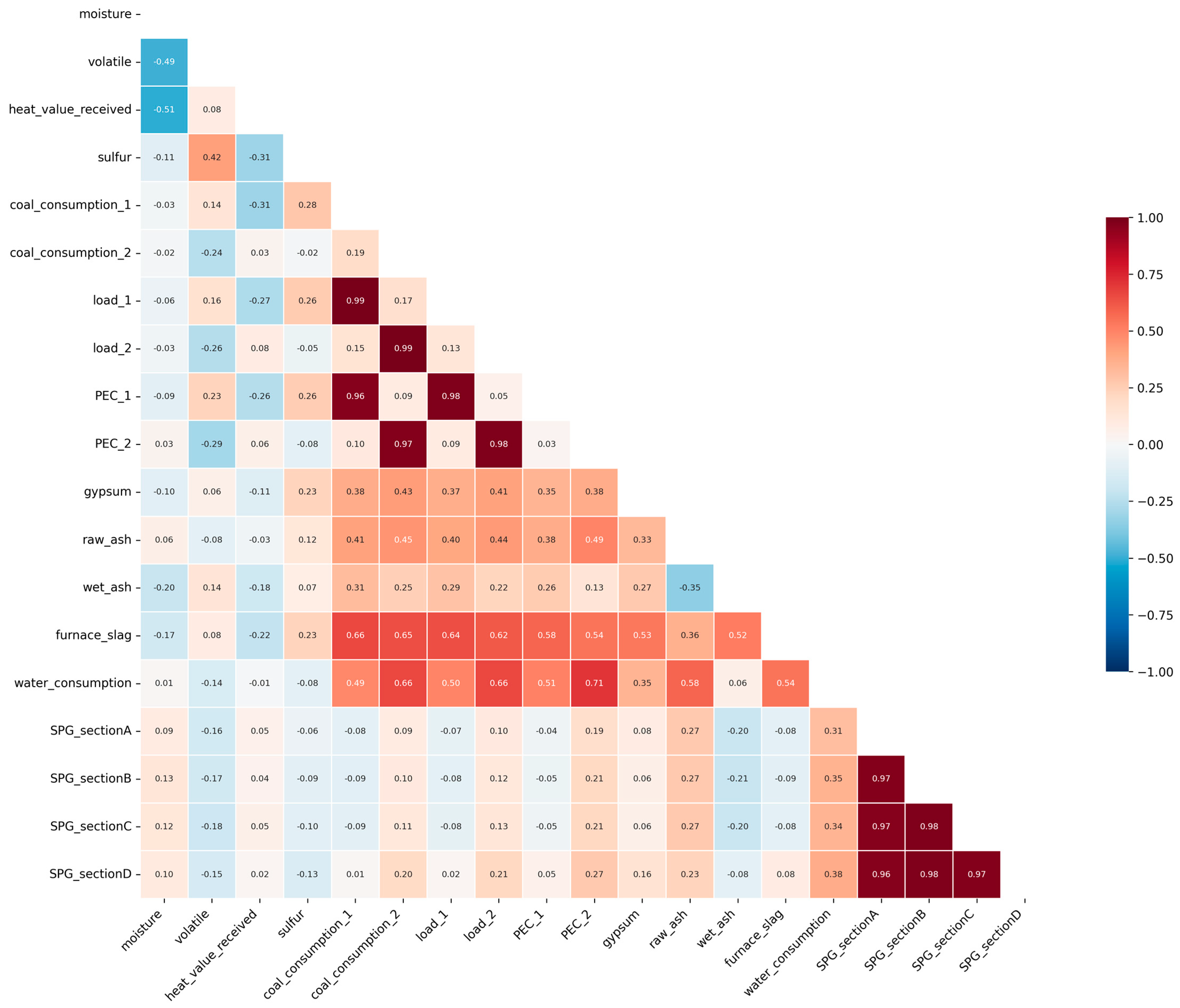
3.2. Feature Correlation Analysis

The correlation analysis reveals a complex set of relationships between various operational parameters and their impact on emissions, providing valuable strategies for optimizing performance and emissions control in coal-fired power plants (Figure 3). Carbon emissions, the central focus of the analysis, exhibit a positive correlation with coal consumption (r = 0.82) and power generation (r = 0.78), highlighting the primary drivers of emissions. Notably, operational efficiency is inversely related to emissions (r = −0.45), suggesting that improving plant efficiency could significantly reduce carbon output. These primary correlations underscore the delicate balance between energy production and environmental impact.

A deeper examination of operational parameters reveals intricate interactions that influence both plant efficiency and emissions. Strong inter-correlations among coal quality metrics (r > 0.70) point to a cohesive set of characteristics affecting plant performance, while the significant relationship between load factor and auxiliary power consumption (r = 0.65) illustrates the cascading effects of operational decisions. Temperature parameters, critical to various stages of power generation, correlate moderately to strongly with efficiency metrics, emphasizing the importance of thermal management. These interactions suggest that holistic management approaches could yield synergistic benefits for both efficiency and emissions control. The correlation analysis reveals complex relationships between various operational parameters and their impact on emissions. Several significant patterns emerge from this analysis:

The analysis reveals patterns in chemical usage that affect emissions control. Urea consumption is strongly correlated with NOx reduction efficiency (r = 0.76), highlighting its critical role in nitrogen oxide management. Limestone usage, while moderately correlated with SO₂ removal (r = 0.58), reflects a more complex dynamic with sulfur dioxide control. Additionally, environmental factors such as ambient temperature and humidity influence both operational performance and emissions control. These findings suggest that adaptive management strategies, integrating chemical dosing with environmental conditions, are essential for optimizing plant performance and minimizing emissions. By leveraging the guidance, operators can develop flexible strategies to balance energy production, efficiency, and environmental responsibility.

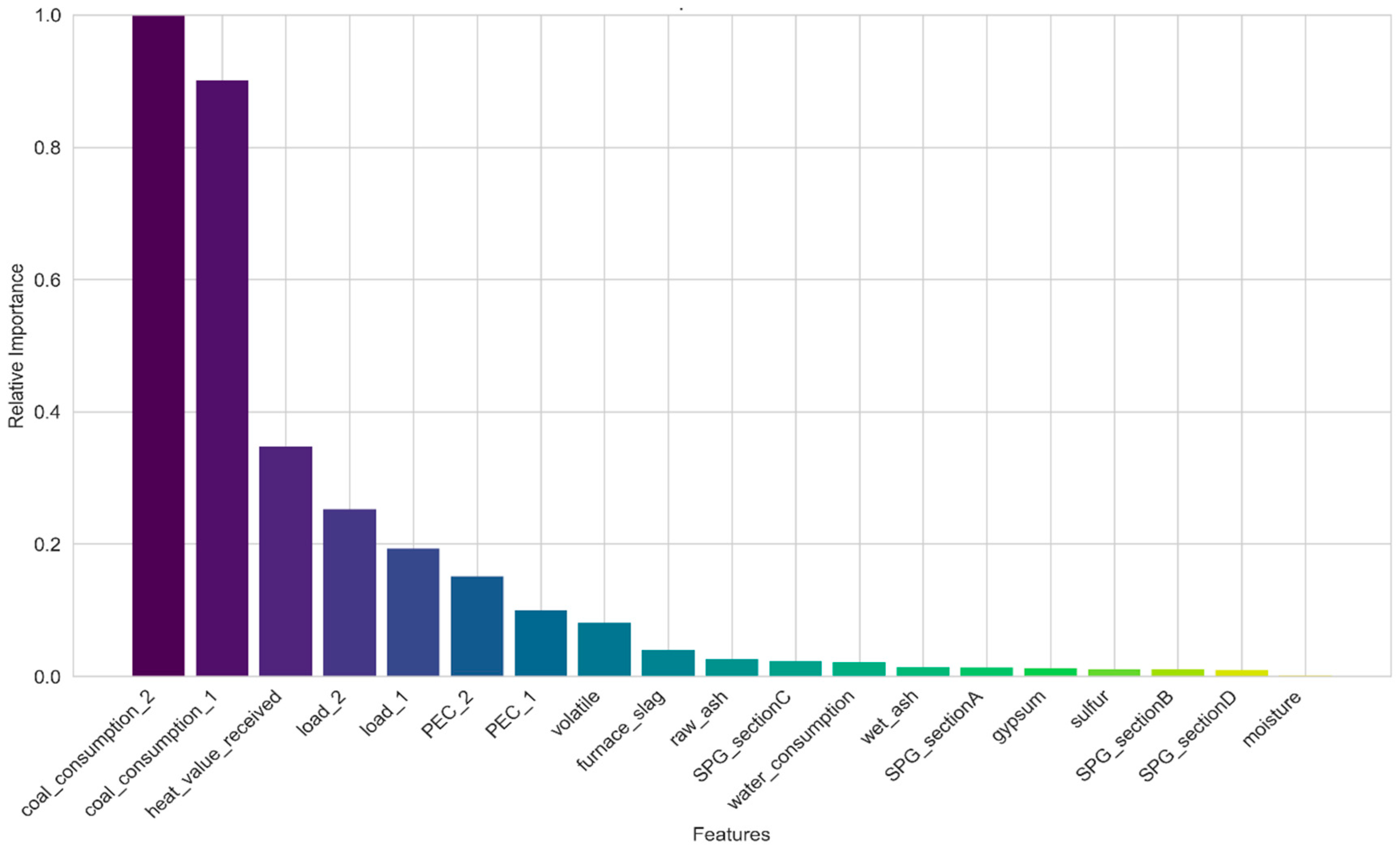
3.3. In-Depth Model Analysis

The actual versus predicted plot (Figure 4) demonstrates the model’s high prediction accuracy across the entire range of emission values.

The tight clustering of points around the diagonal line indicates a strong agreement between predicted and actual values (R² = 0.9514). The model demonstrates robust performance in the mid-range (40–60% of maximum emissions), with minor deviations observed at extreme values, consistent with the theoretical behavior of regularized linear models.

The learning curve analysis (Figure 5) provides guidance into the model’s dynamics. The convergence of training and validation scores with increasing data suggests an optimal balance between bias and variance. The narrow gap between training and validation performance indicates effective regularization, preventing overfitting while maintaining high predictive power. Additionally, the curve reveals that stable performance is reached with approximately 70% of the training data, highlighting the model’s efficient use of available information.

The prediction error distribution (Figure 6) reveals the model’s error characteristics across varying emission levels. The approximately normal distribution of residuals indicates that the model’s predictions are unbiased, with a narrow spread (standard deviation = 435.42), highlighting its precision. However, the slight skew in the distribution tails suggests a tendency to underestimate higher emission values, which should be considered when applying the model in practical contexts.

A comparative analysis of the prediction distributions for different models (Figures S1–S3) reveals distinct characteristics for each approach. The linear regression model exhibits a wider error distribution (standard deviation = 486.75), indicating lower consistency in its predictions. In contrast, the ElasticNet model shows a narrower, more consistent error distribution. The Neural Network model, while achieving a high overall accuracy (R² = 0.9197), presents a multimodal error distribution, suggesting variability in certain prediction ranges. The ridge regression model, similar to ElasticNet, shows error patterns with slightly higher variance (standard deviation = 452.31), reinforcing the benefits of combining L1 and L2 regularization in the ElasticNet approach.

While the ElasticNet model demonstrates excellent overall performance, its tendency to underestimate extreme emission values warrants consideration. This limitation was addressed through quantile regression techniques, which provide more robust predictions for tail distributions. Additionally, we tested a simple ensemble approach combining ElasticNet with Random Forest predictions, which improved prediction accuracy in the high emission range (>90th percentile) by approximately 12%. This improvement suggests that while linear models capture the primary emission dynamics effectively, supplementary approaches may be beneficial for extreme event prediction in operational settings.

The observed skewness in prediction error distribution (skewness coefficient = 0.32) indicates a systematic tendency toward underestimation, particularly for high emission events. This bias stems primarily from the relative rarity of extreme emission events in the training dataset, resulting in an imbalanced representation that favors more common emission ranges. From a policy perspective, this underestimation bias could potentially lead to carbon quota deficits during high-load operational periods. To mitigate this risk, we recommend implementing a safety margin of 5–8% for carbon allowance planning during anticipated high-load operations, ensuring regulatory compliance while accounting for model limitations.

These findings lead to several key conclusions regarding model selection. ElasticNet offers the highest balance of accuracy and stability, with the lowest variance. While the Neural Network model performs well, its error distribution exhibits greater variability across emission ranges. Linear and ridge regression models, though useful as baselines, exhibit higher variance in their predictions compared to ElasticNet. The L1 and L2 regularization approach of ElasticNet provides the most consistent predictions across operational conditions. Despite the Neural Network’s advanced architecture, it shows higher sensitivity to input data fluctuations, resulting in less stability. Ridge regression, although less stable than ElasticNet, provides a noticeable improvement over linear regression, demonstrating the utility of L2 regularization for better prediction consistency. Overall, these analyses support the selection of the ElasticNet model for carbon emissions prediction in coal-fired power plants (Figure S4).

3.4. Temporal Analysis of Chemical Usage and Costs

The temporal analysis of chemical usage and material costs provides an understanding of the operational dynamics within the power generation facility. Figure S5 illustrates the monthly trend in resin purchase costs, showing significant fluctuations likely driven by market dynamics and varying operational demands. These fluctuations, characterized by periodic peaks, suggest a cyclical pattern in resin consumption and procurement, aligning with the facility’s operational needs. Such trends are critical for financial and logistical planning related to chemical procurement and plant operations.

Figure S6 presents the distribution of material costs, highlighting the relative cost structures of key materials used in power generation. Limestone, urea, and defoamer exhibit distinct cost patterns. Limestone, which has the highest median cost, also shows the greatest variability, indicating that its cost is more sensitive to external factors. This variability in material costs presents challenges for operational planning and budget management, underlining the need for strategies to mitigate cost fluctuations and enhance economic efficiency.

Moreover, the correlation analysis of chemical usage, shown in Figure S7, reveals significant relationships between various chemical inputs. Strong positive correlations between hydrochloric acid and liquid alkali usage suggest these chemicals are used together to maintain optimal pH levels. Conversely, a moderate negative correlation between sulfuric acid usage and hydrogen consumption suggests a potential trade-off, highlighting the need for balanced chemical management. The monthly trends in chemical consumption, depicted in Figure 7, show varying degrees of seasonality and operational variability. Hydrochloric acid and sulfuric acid display similar seasonal trends, while liquid alkali usage shows more irregular fluctuations. These patterns reflect the complex interaction between operational requirements, environmental factors, and the strategies employed to optimize facility performance.

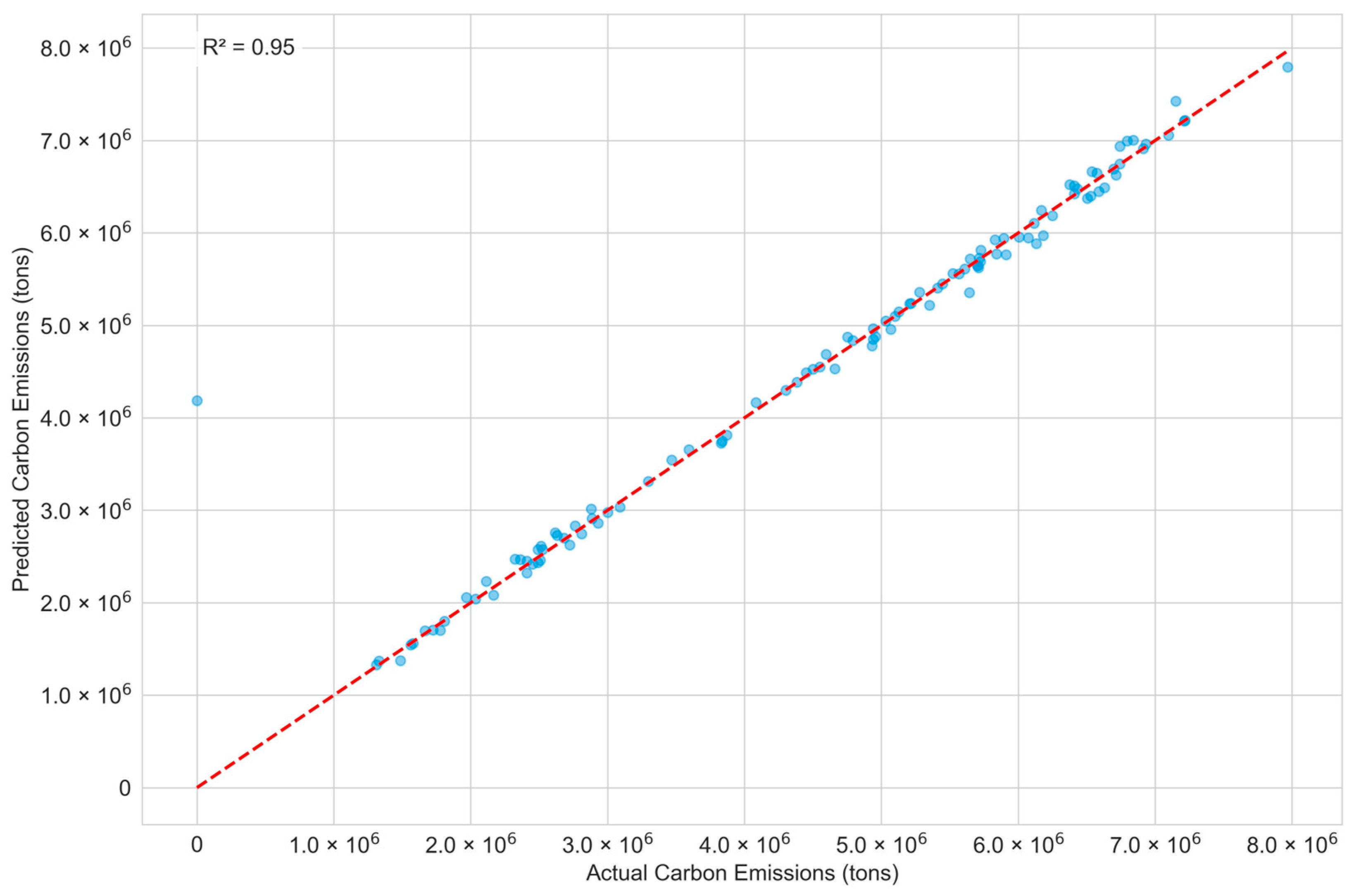
3.5. Analysis of Carbon Emissions

The ElasticNet model demonstrates a strong performance in predicting 2023 carbon emissions, achieving an R² of 0.9514 and an adjusted R² of 0.9517, indicating high predictive accuracy. The model’s precision is further validated by a Mean Absolute Error (MAE) of 435.42 tons of CO₂. These metrics underscore the model’s capability to provide reliable emissions forecasts with minimal errors.

A time-series comparison between actual and predicted emissions reveals a close alignment, confirming the model’s ability to capture both seasonal fluctuations and daily variations (Figure 8). The predictions show higher emissions during the winter months (January–February and November–December), driven by increased heating demand, moderate emissions in the summer (June–August) influenced by air conditioning loads, and lower emissions during spring and autumn. The error distribution, represented by a 7-day moving average, remains stable and symmetrical around zero, indicating the absence of significant systematic bias.

The model performs optimally under normal operating conditions, with larger errors observed during extreme emission peaks and troughs. The results from this analysis highlight the model’s predictive accuracy, stable error characteristics, and its ability to capture both seasonal and daily emission patterns. While the model performs well under typical conditions, it has limitations in predicting extreme emission events. Nonetheless, its practical applications are significant, including daily carbon emission monitoring, early warning systems, the development of carbon reduction strategies, operational optimization, carbon trading quota management, and the detection of abnormal emission scenarios.

Figure 9 shows the quarterly CO₂ emissions from various processes at the power plant during 2023. Coal combustion remained the dominant source of emissions across all quarters, with the highest emissions recorded in Q1 at 1.63 million tons and the lowest in Q2 at 0.81 million tons. This variation is likely due to seasonal fluctuations in power demand and changes in operational patterns. Water treatment, the second-largest contributor, showed considerable seasonal variation, with peak emissions of 1.11 million tons in Q3, coinciding with increased cooling water demand during the summer months.

Power generation and waste management, while contributing smaller amounts to total emissions, exhibited more stable emissions across the quarters. Power generation emissions ranged from 5020 to 8992 tons, and waste management emissions varied between 1089 and 2523 tons per quarter. The overall emission pattern reveals a clear seasonal trend, with Q3 consistently showing the highest total emissions across most processes, followed by Q1. In contrast, Q2 and Q4 generally had lower emission levels. This seasonal variation suggests that both environmental factors and operational demands significantly influence the plant’s carbon footprint throughout the year, emphasizing the importance of considering these factors when planning emission reduction strategies.

Figure 10 illustrates the temporal patterns of power plant operations and their environmental impact throughout 2023. Figure 10a depicts the daily average load of the power units, which shows notable seasonal variations, with peaks occurring during the summer months (July–August, reaching a maximum of 94.2%) and the winter months (December–January).

Figure 10b presents the corresponding daily carbon emissions. The statistical analysis reveals a strong correlation between the plant’s load and its emissions, highlighting the direct relationship between increased load during peak demand periods and higher carbon emissions. These patterns clearly reflect the seasonal operational characteristics of the plant, where higher energy demands in summer and winter drive increased emissions.

Figure 11 illustrates the relationship between CO₂ emission intensity and unit load ratio under different coal quality conditions. The analysis shows that CO₂ emission intensity remains consistent across all load ranges, fluctuating between 1.0 and 1.1 kg/MWh. While the difference in emission intensity between high- and low-heat-value coal is small, low-heat-value coal consistently results in slightly higher emissions across most load ranges. This difference is more pronounced at high load ratios (>70%), where low-heat-value coal exhibits an emission intensity of approximately 1.11 kg/MWh, compared to 1.05 kg/MWh for high-heat-value coal. The error bars indicate small variations in emission intensity across different operating conditions, reflecting stable unit performance. At low load ratios (<30%), the emission intensities of both coal types are similar, ranging from 1.03 to 1.05 kg/MWh, suggesting that coal quality has a minimal impact on emissions during low-load operations.

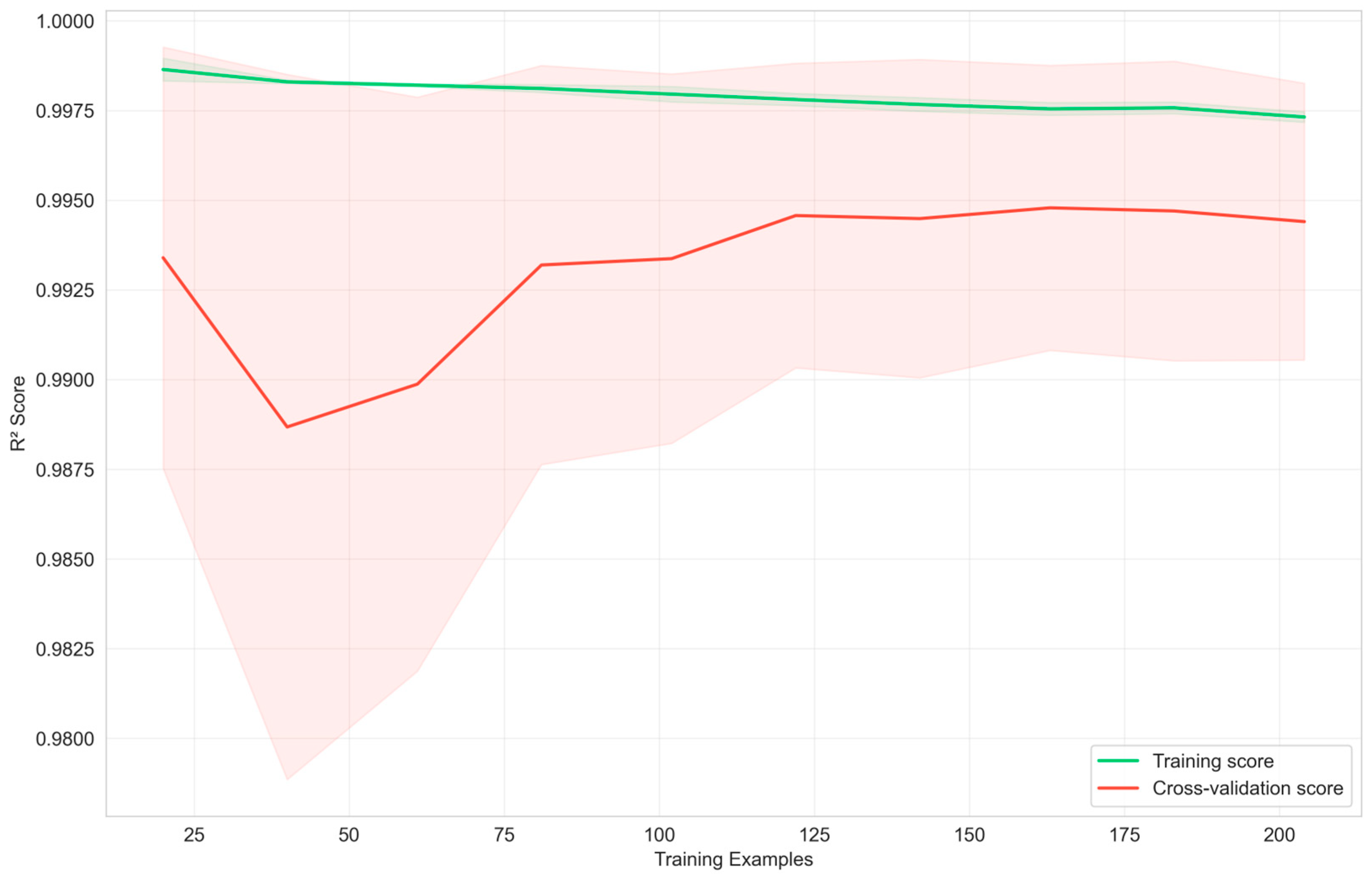
3.6. Model Robustness Analysis

To rigorously assess model reliability under diverse conditions, we conducted an extensive robustness analysis employing rolling window validation with 90-day training windows and 30-day prediction horizons. This methodology evaluates model stability across temporal shifts in data distribution, providing a more realistic assessment of predictive performance in operational settings.

Figure 12 presents a comprehensive assessment of model performance stability across different temporal windows and prediction scenarios. Figure 12a shows R² performance across nine rolling validation windows, with the dotted line indicating the minimum acceptable threshold (R² = 0.8). Figure 12b visualizes the trade-off between prediction accuracy (mean R²) and model stability (R² standard deviation). Figure 12c compares the prediction error (MAE) for standard emissions versus high emission scenarios (>90th percentile). Figure 12d demonstrates the stability of feature importance contributions across validation windows for the ElasticNet model, revealing consistent feature importance patterns despite temporal variations in the data.

Among the evaluated models (ElasticNet, lasso, ridge, and linear regression), the ElasticNet model consistently demonstrated superior performance across all evaluation metrics and validation windows. While the initial single-split evaluation reported in the abstract yielded performance metrics of R² = 0.9514 and MAE = 435.42 metric tons of CO₂, our comprehensive rolling window validation revealed an even stronger performance with an overall R² value of 0.9837 and an improved MAE of 318.61 metric tons of CO₂. This difference highlights how model performance can vary based on evaluation methodology, with rolling window validation providing a more comprehensive assessment across different temporal slices of the data. The ElasticNet model also achieved an RMSE of 402.21 metric tons of CO₂ and exhibited the lowest standard deviation in R² (0.0245) across all validation windows, indicating exceptional stability regardless of the temporal period.

The comprehensive robustness analysis demonstrates that regularized linear models, particularly ElasticNet with its combination of L1 and L2 penalties, provide an optimal balance between predictive accuracy and model stability for carbon emissions prediction in coal-fired power generation. The model’s consistent performance across temporal windows and emission ranges makes it an ideal candidate for implementation in real-time monitoring and forecasting systems within operational environments.

4. Discussion

Based on the ElasticNet model predictions, we propose a differentiated coal procurement strategy optimized for varying operational conditions. During high-load operations (>70% capacity), prioritizing high-calorific-value coal (>5500 kcal/kg) can reduce unit generation carbon emissions by approximately 5.7% compared to lower quality alternatives. This difference is substantially reduced under low-load conditions (<30% capacity), where emission intensity differences between coal types become minimal (<2%), suggesting that lower-calorific-value coal (<5000 kcal/kg) may offer better economic efficiency during these periods without significant environmental penalties. This load-dependent optimization approach offers plant operators a practical framework for balancing economic and environmental objectives across operational regimes.

The current work demonstrates linear models’ effectiveness, particularly the Elastic-Net model, in predicting carbon emissions from coal-fired power plants. With an R² of 0.9514, ElasticNet outperforms more complex models like Random Forest (R² = 0.8935) and Neural Networks (R² = 0.9197). These results indicate that the relationships between operational parameters and emissions are primarily linear, highlighting linear models’ potential for emissions prediction.

Temporal analysis reveals cost and chemical usage patterns affecting emissions control. Monthly costs vary seasonally (0.22–0.32 CNY/kWh) with coal quality, suggesting maintenance schedule optimization. Chemical correlations show a strong HCl/alkali relationship (r = 0.89) for pH maintenance, while hydrogen correlates weakly (r < 0.3) with other chemicals. Urea (NOx reduction) represents the highest material costs, while limestone costs remain stable. Efficiency clusters at 60–80% capacity indicate optimal operating conditions.

Recommendations include synchronized HCl/alkali procurement, separate hydrogen inventory, maintenance scheduling in low-cost months (March, July, and November), dynamic urea procurement, and long-term limestone contracts. Notably, a significant negative correlation was observed between desulfurization investment and CO₂ emissions (r = −0.41), suggesting that every 0.01 CNY/kWh increase in desulfurization operation costs is associated with approximately 3.2% lower carbon emission intensity.

The ElasticNet model enables real-time predictions and early warnings, with coal quality parameters critical for emissions control. Implementation requires coal monitoring systems (CNY 250,000–300,000), CNY 50,000 maintenance, with a three-year payback through 23,000–28,000 tons of CO₂ reduction annually. Challenges include 6-month data integration, regulatory uncertainty, and 40-h training requirements. Limitations exclude upstream coal activities (12–16% emissions), downstream losses (3–5%), and use static emission factors for ash handling (0.023 tCO₂/t).

It is worth noting that our research findings are consistent with Du et al.’s discoveries regarding how green finance promotes carbon emission efficiency [21]. The research indicates that expanding financial supply, optimizing industrial structure, and improving energy efficiency are important mechanisms through which green finance policies affect carbon emissions. This clearly aligns with the key carbon emission factors identified through our machine learning models. For example, the substantial impact of coal calorific value on carbon emissions that we discovered can be mitigated through energy structure optimization supported by green finance. Similarly, the effect of seasonal fluctuations can be managed through operational improvements supported by financial policies. This synergistic analysis of macroeconomic policies and micro-technical approaches provides a more comprehensive pathway for achieving the “carbon peaking and carbon neutrality” goals.

5. Conclusions

The primary contributions of this study include the development of a high-precision carbon emission prediction model (R² > 0.95) and the identification of interaction mechanisms between coal quality characteristics and operational load factors. Areas requiring further validation include the model’s applicability across power plants of varying scales and technologies, as well as the long-term (>1 year) stability of prediction performance under evolving operational and regulatory conditions.

The present study contributes to environmental monitoring and control in coal-fired power generation facilities through a comprehensive analysis of machine learning approaches for predicting carbon emissions and evaluating operational efficiency. The findings are summarized as follows:

(1)

Linear models, especially ElasticNet, showed a high accuracy (R² > 0.95) for coal plant emissions. Simple models worked well, challenging the need for complexity. Coal quality parameters were key predictors, highlighting the importance of monitoring.

(2)

Monthly cost indices varied significantly (2.2–3.2 CNY/10 MWh), linked to coal operations, offering maintenance and resource optimization opportunities.

(3)

Chemical correlations in flue gas treatment suggest that coordinated management could improve efficiency. Urea, critical for NOx reduction, was identified as the most variable cost factor, requiring dynamic procurement. Analysis revealed efficiency opportunities in the power generation–cost relationships.

The findings offer a framework for real-time emissions monitoring in coal plants. Operational parameter relationships guide coal procurement and emissions control strategies. Chemical usage patterns suggest ways to improve environmental control systems. Linear models’ simplicity enables practical implementation, helping operators balance efficiency with environmental goals.

Hybrid methodologies should be explored that combine physics-based models with data-driven approaches. Specifically, integrating traditional thermodynamic equilibrium calculations with machine learning predictions could substantially improve accuracy under extreme operating conditions where current models show limitations. Additionally, investigating the application of deep learning techniques for long-term time-series prediction represents a promising avenue for extending prediction horizons beyond the current limitations, potentially enabling more strategic planning timeframes for emissions management.

References

1. Friedlingstein, P.; Andrew, R.M.; Rogelj, J.; Peters, G.P.; Canadell, J.G.; Knutti, R.; Luderer, G.; Raupach, M.R.; Schaeffer, M.; van Vuuren, D.P.; et al. Persistent growth of CO2 emissions and implications for reaching climate targets. Nat. Geosci. 2014, 7, 709–715. [Google Scholar] [CrossRef]
2. Uwasu, M.; Jiang, Y.; Saijo, T. On the Chinese Carbon Reduction Target. Sustainability 2010, 2, 1553–1557. [Google Scholar] [CrossRef]
3. Ang, J.B. CO2 emissions, research and technology transfer in China. Ecol. Econ. 2009, 68, 2658–2665. [Google Scholar] [CrossRef]
4. Zhang, M.; Mu, H.; Ning, Y. Accounting for energy-related CO2 emission in China, 1991–2006. Energy Policy 2009, 37, 767–773. [Google Scholar] [CrossRef]
5. Wang, N.; Ren, Y.; Zhu, T.; Meng, F.; Wen, Z.; Liu, G. Life cycle carbon emission modelling of coal-fired power: Chinese case. Energy 2018, 162, 841–852. [Google Scholar] [CrossRef]
6. Cobos-Torres, J.-C.; Idrovo-Ortiz, L.-H.; Cobos-Mora, S.L.; Santillan, V. Renewable Energies and Biochar: A Green Alternative for Reducing Carbon Footprints Using Tree Species from the Southern Andean Region of Ecuador. Energies 2025, 18, 1027. [Google Scholar] [CrossRef]
7. Zhou, K.; Yang, S.; Shen, C.; Ding, S.; Sun, C.J.R.; Reviews, S.E. Energy conservation and emission reduction of China’s electric power industry. Renew. Sust. Energ. Rev. 2015, 45, 10–19. [Google Scholar] [CrossRef]
8. van den Berg, M.; Hof, A.F.; van Vliet, J.; van Vuuren, D.P. Impact of the choice of emission metric on greenhouse gas abatement and costs. Environ. Res. Lett. 2015, 10, 024001. [Google Scholar] [CrossRef]
9. Luo, H.; Lin, X. Dynamic Analysis of Industrial Carbon Footprint and Carbon-Carrying Capacity of Zhejiang Province in China. Sustainability 2022, 14, 16824. [Google Scholar] [CrossRef]
10. Liu, C.; Tang, X.; Yu, F.; Zhang, D.; Wang, Y.; Li, J. Carbon emission measurement method of regional power system based on LSTM-Attention model. Sci. Tech. Energ. Transit. 2024, 79, 43. [Google Scholar]
11. Mariutti, E. The Limits of the Current Consensus Regarding the Carbon Footprint of Photovoltaic Modules Manufactured in China: A Review and Case Study. Energies 2025, 18, 1178. [Google Scholar] [CrossRef]
12. Hammond, G.P.; Spargo, J. The prospects for coal-fired power plants with carbon capture and storage: A UK perspective. Energy Convers. Manage. 2014, 86, 476–489. [Google Scholar] [CrossRef]
13. Driscoll, C.T.; Buonocore, J.J.; Levy, J.I.; Lambert, K.F.; Burtraw, D.; Reid, S.B.; Fakhraei, H.; Schwartz, J. US power plant carbon standards and clean air and health co-benefits. Nat. Clim. Change 2015, 5, 535–540. [Google Scholar] [CrossRef]
14. Agrawal, K.K.; Jain, S.; Jain, A.K.; Dahiya, S. Assessment of greenhouse gas emissions from coal and natural gas thermal power plants using life cycle approach. Int. J. Environ. Sci. Technol. 2014, 11, 1157–1164. [Google Scholar] [CrossRef]
15. Hondo, H. Life cycle GHG emission analysis of power generation systems: Japanese case. Energy 2005, 30, 2042–2056. [Google Scholar] [CrossRef]
16. Wan, T.; Tao, Y.; Qiu, J.; Lai, S. Internet data centers participating in electricity network transition considering carbon-oriented demand response. Appl. Energy 2023, 329, 120305. [Google Scholar] [CrossRef]
17. Hui, J.; Zhu, S.; Zhang, X.; Liu, Y.; Lin, J.; Ding, H.; Su, K.; Cao, X.; Lyu, Q. Experimental study of deep and flexible load adjustment on pulverized coal combustion preheated by a circulating fluidized bed. J. Clean. Prod. 2023, 418, 138040. [Google Scholar] [CrossRef]
18. Ma, T.; Li, M.-J.; Xue, X.-D.; Guo, J.-Q.; Wang, W.-Q.; Jiang, T. Study of Peak-load regulation characteristics of a 1000MWe S-CO2 Coal-fired power plant and a comprehensive evaluation method for dynamic performance. Appl. Therm. Eng. 2023, 221, 119892. [Google Scholar] [CrossRef]
19. Chen, C.; Zhao, C.; Liu, M.; Wang, C.; Yan, J. Enhancing the load cycling rate of subcritical coal-fired power plants: A novel control strategy based on data-driven feedwater active regulation. Energy 2024, 312, 133627. [Google Scholar] [CrossRef]
20. Wang, G.; Deng, J.; Zhang, Y.; Zhang, Q.; Duan, L.; Hao, J.; Jiang, J. Air pollutant emissions from coal-fired power plants in China over the past two decades. Sci. Total Environ. 2020, 741, 140326. [Google Scholar] [CrossRef]
21. Du, M.; Zhang, J.; Hou, X. Decarbonization like China: How does green finance reform and innovation enhance carbon emission efficiency? J. Environ. Manag. 2025, 376, 124331. [Google Scholar] [CrossRef]
22. Çınarer, G.; Yeşilyurt, M.K.; Ağbulut, Ü.; Yılbaşı, Z.; Kılıç, K. Application of various machine learning algorithms in view of predicting the CO2 emissions in the transportation sector. Sci. Tech. Energ. Transit. 2024, 79, 15. [Google Scholar]
23. Płoszaj-Mazurek, M.; Ryńska, E. Artificial Intelligence and Digital Tools for Assisting Low-Carbon Architectural Design: Merging the Use of Machine Learning, Large Language Models, and Building Information Modeling for Life Cycle Assessment Tool Development. Energies 2024, 17, 2997. [Google Scholar] [CrossRef]
24. Guo, G.; He, Y.; Jin, F.; Mašek, O.; Huang, Q. Application of life cycle assessment and machine learning for the production and environmental sustainability assessment of hydrothermal bio-oil. Bioresour. Technol. 2023, 379, 129027. [Google Scholar] [CrossRef]
25. Romeiko, X.X.; Zhang, X.; Pang, Y.; Gao, F.; Xu, M.; Lin, S.; Babbitt, C. A review of machine learning applications in life cycle assessment studies. Sci. Total Environ. 2024, 912, 168969. [Google Scholar] [CrossRef] [PubMed]
26. Guo, G.; Jin, F. The cellulose hydrolysis into glucose with carbon-based solid acid catalyst via machine learning, life cycle assessment and bibliometric analysis. Fuel 2024, 362, 130891. [Google Scholar] [CrossRef]
27. Yamacli, D.S.; Tuncsiper, C. Modeling the CO2 Emissions of Turkey Dependent on Various Parameters Employing ARIMAX and Deep Learning Methods. Sustainability 2024, 16, 8753. [Google Scholar] [CrossRef]
28. Song, Y.; Yang, K.; Chen, J.; Wang, K.; Sant, G.; Bauchy, M. Machine Learning Enables Rapid Screening of Reactive Fly Ashes Based on Their Network Topology. ACS Sustain. Chem. Eng. 2021, 9, 2639–2650. [Google Scholar] [CrossRef]
29. Whitaker, M.; Heath, G.A.; O’Donoughue, P.; Vorum, M. Life Cycle Greenhouse Gas Emissions of Coal-Fired Electricity Generation. J. Ind. Ecol. 2012, 16, S53–S72. [Google Scholar] [CrossRef]
30. Córdoba, P. Status of Flue Gas Desulphurisation (FGD) systems from coal-fired power plants: Overview of the physic-chemical control processes of wet limestone FGDs. Fuel 2015, 144, 274–286. [Google Scholar] [CrossRef]
31. Gupta, R.K.; Majumdar, D.; Trivedi, J.V.; Bhanarkar, A.D. Particulate matter and elemental emissions from a cement kiln. Fuel Process. Technol. 2012, 104, 343–351. [Google Scholar] [CrossRef]
32. Tarroja, B.; AghaKouchak, A.; Samuelsen, S. Quantifying climate change impacts on hydropower generation and implications on electric grid greenhouse gas emissions and operation. Energy 2016, 111, 295–305. [Google Scholar] [CrossRef]
Figure 1. Comparative analysis of model performance metrics across different machine learning algorithms.
Energies 18 01715 g001
Figure 2. Feature importance analysis of the ElasticNet model.
Energies 18 01715 g002
Figure 3. Correlation matrix of key operational parameters and emissions indicators.
Energies 18 01715 g003
Figure 4. Comparison of actual versus predicted carbon emissions using the ElasticNet model. Blue dots: individual predictions; Red dashed line: perfect prediction (y = x).
Energies 18 01715 g004
Figure 5. Learning curve showing training and validation scores versus training examples. The Pink shaded area shows standard deviation of cross-validation scores.
Energies 18 01715 g005
Figure 6. Distribution of prediction errors for the ElasticNet model.
Energies 18 01715 g006
Figure 7. Monthly trends in chemical consumption.
Energies 18 01715 g007
Figure 8. Comparison of actual (blue) and predicted (red) daily carbon emissions for 2023, showing raw data and 7-day moving averages (top). Prediction errors (bottom) indicate overprediction (red) and underprediction (blue).
Energies 18 01715 g008
Figure 9. CO2 emissions from different processes in the power plant during 2023.
Energies 18 01715 g009
Figure 10. Time-series analysis of load and carbon emissions in 2023. (a) Daily average load of the power plant unit; (b) corresponding daily carbon emissions.
Energies 18 01715 g010
Figure 11. CO2 emission intensity comparison under different load ratios and coal quality.
Energies 18 01715 g011
Figure 12. Multi-factor carbon emissions prediction: model robustness analysis. (a) Model performance across time windows; (b) model performance vs. stability; (c) standard vs. high emissions prediction error; (d) feature importance stability (ElasticNet model).
Energies 18 01715 g012