A VSG Power Decoupling Control with Integrated Voltage Compensation Schemes

Abstract

Virtual synchronous generator (VSG) control enables grid-connected power electronic converters to retain the inertia support and frequency stability features of traditional synchronous generators in power grids. The power coupling of VSG remains a major issue, where reactive power deviates from the commands. Numerous existing VSG decoupling methods essentially focus on applying virtual impedances in different ways to alter the equivalent line impedance ratio. These methods are less effective under varying operating points. To address the problem, the voltage compensation term from virtual resistance and inductance is first made adaptive to varying operating points through the proposed online parameters’ adjustment. Then, it is further discovered that it is still not possible to achieve total power decoupling for the full operating range. Therefore, an additional voltage compensation term, in terms of the power angle variations, is proposed to eliminate the power coupling at high power ranges. The two proposed voltage compensation schemes are seamlessly integrated so that total VSG power decoupling can be achieved. Through comparative lab tests with existing methods, it is validated that the proposed method is more effective in eliminating reactive power coupling under varying and high-power operating points during both steady and transient states.

1. Introduction

As more distributed energy sources (DESs) are being installed in power systems [1], their power electronic-based grid interfaces, particularly grid-connected converters (GCCs) [2], are taking a large proportion of the power system capacity. Due to the deficiency of voltage and frequency support capability of the GCCs regulated as current sources [3], the total grid inertia and damping are reduced, creating substantial threats to power system stability. This issue has prompted the development of the virtual synchronous generator (VSG) control strategies [4], which enable DESs to emulate the external characteristics of conventional synchronous generators. Despite tremendous research progress in VSG [5], some challenges still remain. A prominent issue is the power coupling between the active power loop (APL) and reactive power loop (RPL) in VSG systems [6] due to their more resistive connection line to low-voltage and low-capacity grids. By comparison, traditional synchronous generators are mostly connected to high-voltage grids, so their line impedance is approximately inductive and negligible power coupling exists [7].

VSG power coupling not only induces significant tracking errors in VSG reactive power [8,9,10] but also reduces power sharing accuracy among multiple VSGs in islanded operation. More critically, as identified in [11], when the line impedance ratio R/X exceeds critical values, VSGs tend to absorb reactive power while delivering active power. This exacerbates grid reactive power shortages, weakens voltage support capability, and reduces power electronic inverter capacity utilization.

To address VSG power coupling issues, scholars have proposed many solutions [12,13,14,15,16,17,18,19,20,21,22,23,24,25]. Some researchers have introduced various voltage compensation techniques to compensate for output reactive power deviations by adjusting the output voltage amplitude, thereby achieving ideal power decoupling [12,13,14]. Nevertheless, these types of VSG power decoupling control studies have not investigated the impacts of varying operating points, which would significantly deteriorate power decoupling performance.

Intelligent algorithms have also been used to tackle VSG decoupling tasks under uncertain line impedance conditions. In [15], an online-trained adaptive fuzzy neural network power decoupling (AFNNPD) strategy for VSG control is proposed. Paper [16] presents an adaptive optimal control method for VSG through reinforcement learning and adaptive dynamic programming (ADP). However, these approaches are hard to implement in practical applications and they have not investigated the impacts of varying operating points as well.

So far, most VSG decoupling studies are from the perspective of applying virtual impedance in different ways. Early papers introduced a virtual inductor (VI) method, which alters the voltage commands when an inductor’s voltage drops [17,18,19,20], making equivalent line impedance more inductive. However, their decoupling effectiveness is limited, as the virtual inductor is essentially different than physical inductors in power decoupling mechanisms. An attempt to address the issue is made in [21] (QVPDC), where the d-axis voltage component produced by a virtual inductor is eliminated to enhance power decoupling. Nevertheless, transient power fluctuations exist during power output variations.

A negative virtual resistor is added to virtual impedance in [22,23,24] in order to further enhance the power decoupling effectiveness by directly eliminating the impact of line resistance for a more inductive equivalent line. In [22], virtual impedance is implemented by replacing the VSG voltage control loop with virtual admittance instead of the usual way of altering voltage commands to the voltage–current double loops of VSG control. Paper [23] proposes to fix virtual impedance values over frequency ranges in order to stabilize the virtual voltage drops over the virtual impedance at all frequencies, improving VSG system stability. Meanwhile, in [24], it is further introduced that virtual impedances are configured differently for harmonic frequencies to further improve the quality of the output current.

A virtual capacitor is proposed to be added to virtual impedance in [25], where it is called virtual inductor and virtual capacitor (VIVC) decoupling control. Moreover, both steady-state and transient power decoupling are investigated in this paper. However, the inclusion of virtual capacitors does have its side effect; for example, the virtual capacitors would add an unwanted initial VSG voltage during the startup of the VSG grid connection, even with zero command. Therefore, undesired reactive power would be induced during grid connection. This side effect is also verified by lab tests in this paper.

In summary, these existing voltage compensation-based methods and the virtual impedance type of methods have not investigated power decoupling performance under varying operating points, which would seriously deteriorate power decoupling performance. In other words, virtual resistance and virtual inductances are not dynamically adjusted to maintain the total power decoupling.

To address these issues, this paper made the following contributions.

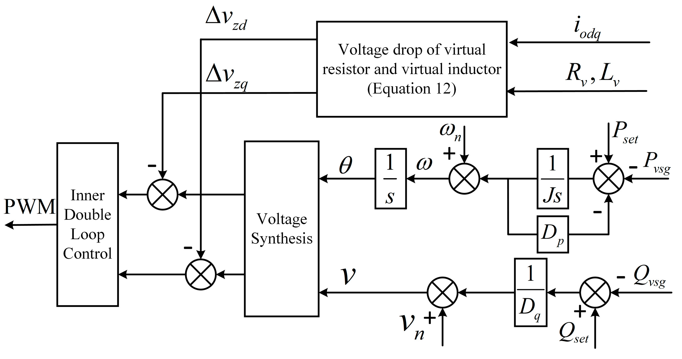
• It introduces the voltage compensation term from virtual resistance and inductance, which are made adaptive to varying operating points by the proposed online parameter adjustments.
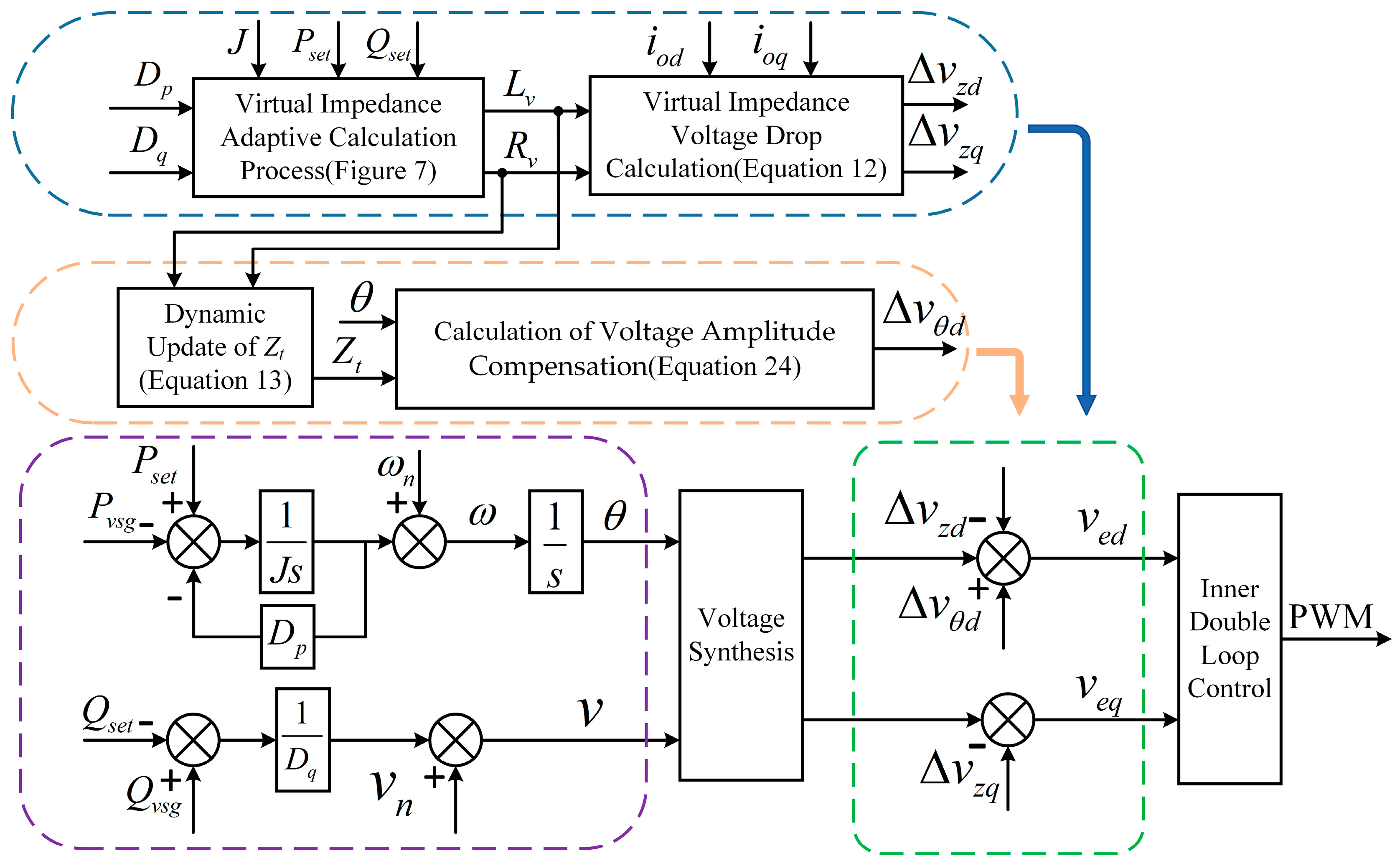
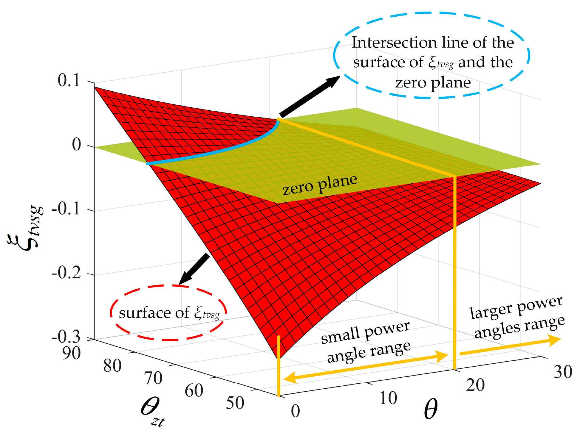
• It is further discovered that total power decoupling limits the full operating range. Therefore, an additional voltage compensation term, Δv_θd, in terms of power angle variations, is proposed to eliminate the power coupling at high power ranges.
• The two proposed voltage compensation schemes are seamlessly integrated so that total VSG power decoupling can be achieved.

The paper is organized as follows. Section 2 introduces the fundamental principle of VSG control and establishes small-signal power models. Herein, the power coupling mechanism is analyzed and both steady-state and transient coupling coefficients are defined for quantitative power coupling evaluation. In Section 3, an adaptive virtual impedance method, with its parameter selection process for virtual inductor and resistor, is first proposed to produce the voltage compensation term. Herein, optimal virtual inductors and resistors are dynamically adjusted online to obtain total decoupling coefficients for both steady-state and transient state under varying power outputs. It is further discovered that total power decoupling is not achievable for the full operating range, especially at high power ranges. Then, an additional voltage compensation term, Δv_θd, in terms of the power angle variations, is derived and integrated with the first part of the voltage compensation produced by the adaptive virtual impedances. Section 4 validates the effectiveness of the proposed power decoupling strategy through comparative lab tests. Finally, Section 5 concludes the paper with its key contributions and findings.

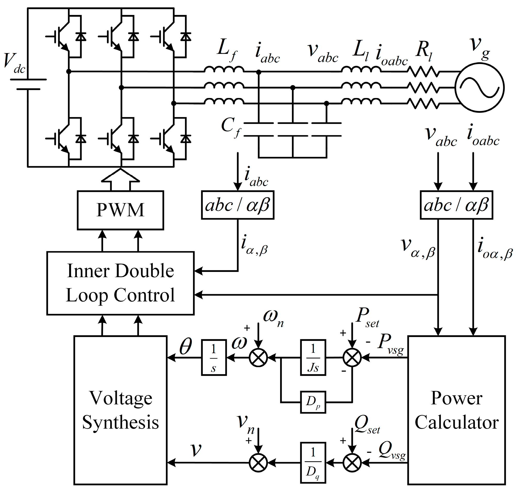
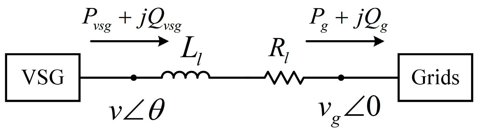
2. VSG Model and Power Coupling Analysis

The basic control block diagram of the VSG is shown in Figure 1, where the DC power supply is connected to the AC grid through a three-phase voltage source type inverter. In Figure 1, L_f, C_f, L_l, and R_l are the filter inductor, the filter capacitor, the line inductor, and the line resistor, respectively. i_abc, v_abc, i_oabc, and v_g are the current of the inverter side, the output voltage of the filter capacitor, the current of the net side, and the voltage of the AC grid, respectively. The control system consists of two parts, namely the power loop and the inner double loop. The active power loop of the power loop gives the amplitude of the reference voltage, and the reactive power loop gives the real-time phase of the reference voltage. The internal voltage–current double closed loop control part is responsible for tracking the output of the power loop. The mathematical expression for VSG control can be given by Figure 1 as

$$\left\{\begin{array}{c}{P}_{set}-P_{vsg}-D_p(\omega -{\omega }_n)=J_p{\displaystyle \frac{d(\omega -{\omega }_n)}{dt}}\\ Q_{set}-Q_{vsg}=D_q(v-v_n)\end{array}\right.,$$

(1)

where P_set, Q_set, P_vsg, and Q_vsg are the given active and reactive power reference values, actual output, and active and reactive power; D_p, J, and D_q are droop coefficients of active loop, virtual inertia coefficients, and droop coefficients of reactive loop, respectively; ω_n, ω, v_n, and v are the rated angular frequency and actual angular frequency of the output voltage, the rated output voltage, and the actual output voltage. The VSG control system can be simplified to the circuit diagram in Figure 2.

In Figure 2, P_g and Q_g are the active and reactive power absorbed by the grid, P_vsg and Q_vsg are the active and reactive power generated at the VSG side, and θ is the power angle between the inverter output voltage v∠θ and the grid voltage v_g∠0. The equivalent line impedance Z_l can be shown as

$$Z_l=R_l+j\omega L_l.$$

(2)

The mathematical expressions for P_vsg, Q_vsg can be obtained by Figure 2 as

$$\left\{\begin{array}{c}{P}_{vsg}={\displaystyle \frac{v^2}{Z_l}}\cos {\theta }_{zl}-{\displaystyle \frac{v{v}_g}{Z_l}}\cos ({\theta }_{zl}+\theta )\\ Q_{vsg}={\displaystyle \frac{v^2}{Z_l}}\sin {\theta }_{zl}-{\displaystyle \frac{v{v}_g}{Z_l}}\sin ({\theta }_{zl}+\theta )\end{array}\right.,$$

(3)

where θ_zl is the line impedance angle and Z_l is the line impedance combining L_l and R_l. The small-signal model of the VSG output power can be obtained after linearization of Equation (3) as

$$\left[\begin{array}{c}\Delta P_{vsg}\\ \Delta Q_{vsg}\end{array}\right]=\left[\begin{array}{cc}{n}_{11}& n_{12}\\ n_{21}& n_{22}\end{array}\right]\left[\begin{array}{c}\Delta \theta \\ \Delta v\end{array}\right],$$

(4)

where

$$\left\{\begin{array}{l}{n}_{11}={\displaystyle \frac{v_0{v}_g}{Z_l}}\sin ({\theta }_{zl}+{\theta }_0)\hfill \\ n_{12}={\displaystyle \frac{2v_0}{Z_l}}\cos {\theta }_{zl}-{\displaystyle \frac{v_g}{Z_l}}\cos ({\theta }_{zl}+{\theta }_0)\hfill \\ n_{21}=-{\displaystyle \frac{v_0{v}_g}{Z_l}}\cos ({\theta }_{zl}+{\theta }_0)\hfill \\ n_{22}={\displaystyle \frac{2v_0}{Z_l}}\sin {\theta }_{zl}-{\displaystyle \frac{v_g}{Z_l}}\sin ({\theta }_{zl}+{\theta }_0)\hfill \end{array}\right.,$$

(5)

where θ₀ is the steady-state power angle and v₀ is the steady-state output voltage of VSG.

Since the active power of VSG is ideally only related to the power angle and the reactive power is ideally only related to the voltage, it is seen from Equation (4) that there are coupling terms (n₁₂Δv, n₂₁Δθ) between active and reactive powers in the VSG small-signal model. It can be further seen from n₁₂ and n₂₁ in Equation (5) that when the sum of θ₀ and θ_zl is not 90°, n₂₁ is not 0. Then, as the indicator for active power, Δθ will produce an undesired amount of ΔQ_vsg. When the line impedance angle is relatively high and the power angle is relatively small (θ₀ ≈ 0), n₁₂ and n₂₁ are about 0. Therefore, power coupling is due to the effects of both θ_zl and θ₀.

To quantify the severity of power coupling with comprehensive considerations of these two contributing factors, the steady-state coupling coefficient ξ_vsg is defined here as the ratio of ΔQ_vsg to ΔP_vsg. To obtain such a ratio, the Δv term in Equation (4) is first to be substituted in terms of ΔQ_vsg, which can be expressed as

$$\Delta v=-{\displaystyle \frac{1}{D_q}}\Delta Q_{vsg}.$$

(6)

After such substitution, Equation (4) can be simplified as

$$\left\{\begin{array}{c}\Delta P_{vsg}=n_{11}\Delta \theta -{\displaystyle \frac{n_{12}}{D_q}}\Delta Q_{vsg}\\ \Delta Q_{vsg}=n_{21}\Delta \theta -{\displaystyle \frac{n_{22}}{D_q}}\Delta Q_{vsg}\end{array}\right..$$

(7)

Then, ξ_vsg can be derived from Equation (7) as

$$\begin{array}{c}{\xi }_{vsg}={\displaystyle \frac{\Delta Q_{vsg}}{\Delta P_{vsg}}}={\displaystyle \frac{1}{\frac{n_{11}}{n_{21}}(1+\frac{n_{22}}{D_q})-\frac{n_{12}}{D_q}}}\\ \hspace{1em}\hspace{1em}\hspace{1em} ={\displaystyle \frac{D_q\cos ({\theta }_{zl}+{\theta }_0)}{\frac{v_g}{Z_l}-\frac{2v_0}{Z_l}\cos {\theta }_0-D_q\sin ({\theta }_0+{\theta }_{zl})}}\end{array}.$$

(8)

Moreover, the severity of transient power coupling when switching between different operating points also needs to be defined as the transient coupling coefficient. As for a multiple-input–multiple-output (MIMO) system, as in Equation (4), the relative gain matrix (RGA) is commonly used to evaluate dynamic system coupling by the ratio of the open-loop gain to the closed-loop gain between the inputs and outputs of the system. Specifically, for reactive power coupling, it is to be determined how much the response of input Δv to the output ΔQ_vsg is coupled by other variables in the MIMO system in Equation (4).

The open-loop gain p₁₁ from Δv to ΔQ_vsg is the direct control effect of Δv on ΔQ_vsg by setting Δθ = 0 in Equation (4) as

$$p_{11}=n_{22}.$$

(9)

The closed-loop gain q₁₁ from Δv to ΔQ_vsg also includes the effect of Δθ on ΔQ_vsg, while ΔP_vsg is controlled in a closed loop to make ΔP_vsg = 0 in Equation (4), from which the closed-loop gain q₁₁ can be derived as

$$q_{11}={\displaystyle \frac{n_{11}{n}_{22}-n_{12}{n}_{21}}{n_{11}}}.$$

(10)

Then, the transient power coupling coefficient is obtained as ρ₁₁ at the first column and first row of the relative gain matrix, which is the ratio of the open-loop gain p₁₁ to the closed-loop gain q₁₁ as

$${\rho }_{11}={\displaystyle \frac{p_{11}}{q_{11}}}={\displaystyle \frac{n_{11}{n}_{22}}{n_{11}{n}_{22}-n_{12}{n}_{21}}},$$

(11)

where the n₁₁-n₂₂ term comes from Equation (5). As for reactive power transient coupling, when ρ₁₁ is 1, the response of input Δv to the output ΔQ_vsg is ideally decoupled from other variables in the MIMO system in Equation (4).

With the VSG system parameters in

Table 1. Analytical and Experimental Parameters.

Symbol	Parameter	Value
Vdc	DC voltage	700 V
Vn	Normal value of line voltage	380 V
Sn	Normal value of power	30 kVA
fn	Normal value of frequency	50 Hz
fsw	Switching frequency	15 kHz
Lf	Inductor of LC filter	300 μH
Cf	Capacitor of LC filter	25 μF
Ll	Inductor of the line	1600 μH
Rl	Resistor of the line	0.5 Ω
Vg	Rated voltage of grid	380 V
Dp	Droop coefficient of active power loop	10,000 W*s/rad
Dq	Droop coefficient of reactive power loop	2000 A
J	The inertial coefficient of active power loop	10 W*s2/rad

, the steady-state coupling coefficient ξ_vsg and transient coupling coefficient ρ₁₁ are plotted with varying line resistances in Figure 3a and Figure 3b, respectively. As the line resistance decreases, the steady-state and transient coupling coefficients approach 0 and 1, respectively. Figure 3c shows the VSG system simulation results with an active power step command of 10 kW with three different line resistances selected at A, B and C, as in Figure 3a,b. These three line resistances are selected here just to have sufficient differences in the resulting coupling coefficients, so that the time domain simulation in Figure 3c will display large enough differences in their reactive power coupling. With higher ξ_vsg and ρ₁₁, both the steady-state reactive power deviations and the transient reactive power overshoots increase, as shown in Figure 3c.

3. Proposed VSG Power Decoupling Control with Integrated Voltage Compensation Schemes

As the effectiveness of the existing VSG power decoupling methods are limited under varying operating points, this paper first proposes an online parameter-adjustment-based voltage compensation method to make virtual resistance and inductance adaptive to varying operating points.

3.1. Proposed Voltage Compensation by Adaptive Virtual Impedance Control

Herein, the first voltage compensation term from virtual resistance and inductance is illustrated as in Figure 4.

In Figure 4, the voltage drops of virtual impedance in the dq-axis, Δv_zd and Δv_zq, are calculated as

$$\left\{\begin{array}{l}\Delta v_{zd}=-\omega L_v{i}_{oq}-R_v{i}_{od}\hfill \\ \Delta v_{zq}=\omega L_v{i}_{od}-R_v{i}_{oq}\hfill \end{array}\right..$$

(12)

The equivalent line impedance after using the virtual impedance method can be adapted from Equation (2) as

$$Z_t=R_l-R_v+j\omega (L_l+L_v).$$

(13)

Then, the output powers after applying the virtual impedances are derived as

$$\left\{\begin{array}{c}{P}_{vsg}={\displaystyle \frac{v^2}{Z_t}}\cos {\theta }_{zt}-{\displaystyle \frac{v{v}_g}{Z_t}}\cos ({\theta }_{zt}+\theta )+i_o^2{R}_v\\ Q_{vsg}={\displaystyle \frac{v^2}{Z_t}}\sin {\theta }_{zt}-{\displaystyle \frac{v{v}_g}{Z_t}}\sin ({\theta }_{zt}+\theta )-i_o^2{X}_v\end{array}\right.,$$

(14)

where θ_zt is the equivalent line impedance angle after adding the virtual impedance and i_o is the amplitude of the output current, which can be derived from Figure 2 as follows:

$$i_o=\sqrt{{\displaystyle \frac{v^2+v_g^2-2v{v}_g\cos \theta }{Z_t^2}}}.$$

(15)

With virtual impedance applied, the output power small-signal equation can be derived as

$$\left[\begin{array}{c}\Delta P_{vsg}\\ \Delta Q_{vsg}\end{array}\right]=\left[\begin{array}{cc}{m}_{11}& m_{12}\\ m_{21}& m_{22}\end{array}\right]\left[\begin{array}{c}\Delta \theta \\ \Delta v\end{array}\right],$$

(16)

where

$$\left\{\begin{array}{l}{m}_{11}={\displaystyle \frac{v_0{v}_g}{Z_t}}\sin ({\theta }_{zt}+{\theta }_0)+{\displaystyle \frac{2v_0{v}_g{R}_v}{Z_t^2}}\sin {\theta }_0\hfill \\ m_{12}={\displaystyle \frac{2v_0}{Z_t}}\cos {\theta }_{zt}-{\displaystyle \frac{v_g}{Z_t}}\cos ({\theta }_{zt}+{\theta }_0)+{\displaystyle \frac{2v_0{R}_v}{Z_t^2}}-{\displaystyle \frac{2v_g{R}_v}{Z_t^2}}\cos {\theta }_0\hfill \\ m_{21}=-{\displaystyle \frac{v_0{v}_g}{Z_t}}\cos ({\theta }_{zt}+{\theta }_0)-{\displaystyle \frac{2v_0{v}_g{X}_v}{Z_t^2}}\sin {\theta }_0\hfill \\ m_{22}={\displaystyle \frac{2v_0}{Z_t}}\sin {\theta }_{zt}-{\displaystyle \frac{v_g}{Z_t}}\sin ({\theta }_{zt}+{\theta }_0)-{\displaystyle \frac{2v_0{X}_v}{Z_t^2}}+{\displaystyle \frac{2v_g{X}_v}{Z_t^2}}\cos {\theta }_0\hfill \end{array}\right.$$

(17)

Next, it is proposed that the virtual impedance parameters are made adaptive to enable online adjustment. This online parameter selection process is based on the steady-state and transient power coupling coefficients defined in Section 2. However, with the virtual impedances applied, the steady-state coupling coefficients are derived as

$$\begin{array}{cc}{\xi }_{tvsg}& ={\displaystyle \frac{\Delta Q_{vsg}}{\Delta P_{vsg}}}={\displaystyle \frac{1}{\frac{m_{11}}{m_{21}}(1+\frac{m_{22}}{D_q})-\frac{m_{12}}{D_q}}}\hfill \\ & ={\displaystyle \frac{(-Z_t^2\cos ({\theta }_{zt}+{\theta }_0)-2Z_t{X}_v\sin {\theta }_0)D_q}{(Z_t^2\sin ({\theta }_{zt}+{\theta }_0)+2Z_t{R}_v\sin {\theta }_0)D_q+v_0(2Z_t\cos {\theta }_0+4F-2G)+v_g(2E-Z_t)}}\hfill \end{array},$$

(18)

where

$$\left\{\begin{array}{l}E=(R_v\cos {\theta }_{zt}-X_v\sin {\theta }_{zt})\\ F=\sin {\theta }_0(R_v\sin {\theta }_{zt}+X_v\cos {\theta }_{zt})\\ G=(X_v\sin ({\theta }_{zt}+{\theta }_0)-R_v\cos ({\theta }_{zt}+{\theta }_0))\end{array}\right..$$

(19)

To illustrate the impact of the virtual impedance parameters on the steady-state coupling coefficient, ξ_tvsg is plotted in Figure 5 under different operating points, with P_set being 10 kW, 15 kW, and 20 kW. It can be seen that the curvy plane of steady-state coupling coefficient ξ_tvsg, for each operating point, cuts across the zero plane. This indicates that by selecting the appropriate virtual resistor and virtual inductor, ξ_tvsg can be made 0 and total reactive power decoupling can be achieved. On the other hand, it shows the necessity to have different virtual impedances based on different operating points in order to make ξ_tvsg 0. This then makes the first step in this proposed online adaptive calculation process to obtain the virtual resistor and virtual inductor.

In Figure 5, it is observed that for each operating point, there is a group of virtual inductor and resistor values where ξ_tvsg is zero. Therefore, the optimal virtual impedance value with the transient coupling coefficients closer to 1 can be further selected from this group. With additional virtual inductor and resistor, the transient coupling coefficient ρ₁₁ is calculated as

$${\rho }_{11}={\displaystyle \frac{m_{11}{m}_{22}}{m_{11}{m}_{22}-m_{12}{m}_{21}}}$$

(20)

With Equation (20), the transient coupling coefficients ρ₁₁ of all the virtual impedance values with zero ξ_tvsg, as in Figure 5, can be obtained for the three operating points (10 kW, 15 kW, and 30 kW) and plotted in Figure 6. Among each group of virtual impedances for each operating point (same color), the optimal virtual impedance value with the transient coupling coefficients closer to 1 can be selected as circled in Figure 6.

Given any operating point of active and reactive power commands, the two-step virtual impedance parameters’ selection process, as illustrated in Figure 5 and Figure 6, is summarized in Figure 7. In the first step, Equation (18) is used as the steady-state coupling selection criteria to obtain all R_v and L_v with ξ_vsg = 0 online, which is then screened by Equation (20) to find the R_v, and L_v with the transient selection criteria ρ₁₁ closer to 1. The virtual impedance parameters selected through this two-step process, as in Figure 7, achieve VSG power decoupling in both the steady state and the transient state.

The virtual resistance and inductance online adjustment process, as illustrated in Figure 7, might not always find parameters to make ξ_tvsg zero. This limitation can be exemplified by Figure 8, which illustrates the variation of ξ_tvsg under the operating range with the power angle from 0° to 30° and the equivalent line impedance angle θ_zt from 45° to 90°. Herein, when the power angle is within a sufficiently small range, ξ_tvsg can be make zero at the intersection line of the surface of ξ_tvsg and the zero plane, as marked in Figure 8. This can be achieved by adjusting θ_zt via the priorly proposed online adjustment of the virtual resistance and inductance. In this particular case, this small power angle range encompasses the power angles under 20°, as marked in Figure 8. However, for a larger power-angle range, like the power angles above 20° in this case, the surface of ξ_tvsg will not intersect the zero plane, even when θ_zt is extended to its full range. It is also obvious from Figure 8 that the deviation of the surface of ξ_tvsg from the zero plane shows a positive correlation with the power angle values.

3.2. Integation of Additional Voltage Compensation Term for Power Angle Variations

So far, even though the voltage compensation term from the virtual resistance and inductance has been made more adaptive to varying operating points by the proposed online parameters adjustment, it is still not possible to achieve total power decoupling for the full operating range, especially at high power ranges. Therefore, it is also necessary to add an additional voltage compensation term Δv_θd in terms of power angle variations.

To derive Δv_θd, the reactive power small-signal equation is first extracted from Equations (16) and (17) as

$$\Delta Q_{vsg}=m_{21}\Delta \theta +m_{22}\Delta v,$$

(21)

which is further expanded as

$$\begin{array}{c}\Delta Q_{vsg}=({\displaystyle \frac{v_0{v}_g}{Z_t}}\sin {\theta }_0-{\displaystyle \frac{2v_0{v}_g{X}_v}{Z_t^2}}\sin {\theta }_0)\Delta \theta \\ \hspace{1em}\hspace{1em}\hspace{1em}\hspace{1em}\hspace{1em}\hspace{1em}\hspace{1em}\hspace{1em}+({\displaystyle \frac{2v_0}{Z_t}}-{\displaystyle \frac{2v_0{X}_v}{Z_t^2}}-{\displaystyle \frac{v_g}{Z_t}}\cos {\theta }_0+{\displaystyle \frac{2v_g{X}_v}{Z_t^2}}\cos {\theta }_0)\Delta v\end{array},$$

(22)

where ΔQ_vsg can be further substituted by Δv according to Equation (6) as

$$\begin{array}{c}-D_q\Delta v=({\displaystyle \frac{v_0{v}_g}{Z_t}}\sin {\theta }_0-{\displaystyle \frac{2v_0{v}_g{X}_v}{Z_t^2}}\sin {\theta }_0)\Delta \theta \\ \hspace{1em}\hspace{1em}\hspace{1em}\hspace{1em}\hspace{1em}\hspace{1em}\hspace{1em}\hspace{1em} +({\displaystyle \frac{2v_0}{Z_t}}-{\displaystyle \frac{2v_0{X}_v}{Z_t^2}}-{\displaystyle \frac{v_g}{Z_t}}\cos {\theta }_0+{\displaystyle \frac{2v_g{X}_v}{Z_t^2}}\cos {\theta }_0)\Delta v\end{array}.$$

(23)

By redefining the voltage amplitude derivation Δv in Equation (23) as the additional voltage compensation term Δv_θd, Equation (23) can then be reorganized as

$$\Delta v_{\theta d}={\displaystyle \frac{v_0{v}_g\sin {\theta }_0(Z_t-2X_v)}{D_q{Z}_t^2+2v_0(Z_t-X_v)+v_g\cos {\theta }_0(2X_v-Z_t)}}\Delta \theta ,$$

(24)

where θ₀ is calculated from Equation (3) as

$${\theta }_0={\displaystyle \frac{1}{2}}\arcsin {\displaystyle \frac{2P_{vsg}{Z}_t}{3v_g^2}}.$$

(25)

This additional voltage compensation term Δv_θd, as proposed in Equation (24), is to be added to Figure 4, where there is the first voltage compensation term from virtual resistance and inductance with an online adjustment. Meanwhile, this adaptive set of virtual resistance and inductance (Z_t) during the process of obtaining the first voltage compensation term is also needed for computing the second voltage compensation term Δv_θd. Therefore, the overall control block diagram of the proposed integrated voltage compensation schemes is shown in Figure 9.

In Figure 9, the reference voltages integrating both voltage compensation terms are expressed as

$$\left\{\begin{array}{l}{v}_{ed}=v-\Delta v_{zd}+\Delta v_{\theta }\hfill \\ v_{eq}=-\Delta v_{zq}\hfill \end{array}\right..$$

(26)

After the proposed method integrates the first compensation voltage from the virtual impedance adaptive to varying operating points and the second voltage compensation term in terms of power angle variations, the steady-state and transient coupling coefficients can then be derived again to investigate the resulting improvement. With two proposed voltage compensation terms, the output power of VSG is derived as

$$\left\{\begin{array}{c}{P}_{vsg}={\displaystyle \frac{{(v+k\theta )}^2}{Z_t}}\cos {\theta }_{zt}-{\displaystyle \frac{(v+k\theta )v_g}{Z_t}}\cos ({\theta }_{zt}+\theta )+i_o^2{R}_v\\ Q_{vsg}={\displaystyle \frac{{(v+k\theta )}^2}{Z_t}}\sin {\theta }_{zt}-{\displaystyle \frac{(v+k\theta )v_g}{Z_t}}\sin ({\theta }_{zt}+\theta )-i_o^2{X}_v\end{array}\right..$$

(27)

By linearizing the operating point, the output power small-signal equation can be derived as

$$\left[\begin{array}{c}\Delta P_{vsg}\\ \Delta Q_{vsg}\end{array}\right]=\left[\begin{array}{cc}{t}_{11}& t_{12}\\ t_{21}& t_{22}\end{array}\right]\left[\begin{array}{c}\Delta \theta \\ \Delta v\end{array}\right],$$

(28)

where

$$\left\{\begin{array}{c}{t}_{11}={\displaystyle \frac{v_0{v}_g\sin ({\theta }_{zt}+{\theta }_0)-k{v}_g\cos ({\theta }_{zt}+{\theta }_0)+2k{v}_0\cos {\theta }_{zt}}{Z_t}}\\ +{\displaystyle \frac{2v_0{v}_g{R}_v\sin {\theta }_0-2k{v}_g{R}_v\cos {\theta }_0+2k{v}_0}{Z_t^2}}\hspace{1em}\hspace{1em}\hspace{1em}\hspace{1em}\\ t_{12}={\displaystyle \frac{2v_0\cos {\theta }_{zt}-v_g\cos ({\theta }_{zt}+{\theta }_0)}{Z_t}}+{\displaystyle \frac{2v_0{R}_v-2v_g{R}_v\cos {\theta }_0}{Z_t^2}}\\ t_{21}={\displaystyle \frac{-v_0{v}_g\cos ({\theta }_{zt}+{\theta }_0)-k{v}_g\sin ({\theta }_{zt}+{\theta }_0)+2k{v}_0\sin {\theta }_{zt}}{Z_t}}\\ +{\displaystyle \frac{-2v_0{v}_g{X}_v\sin {\theta }_0+2k{v}_g{X}_v\cos {\theta }_0-2k{v}_0}{Z_t^2}}\hspace{1em}\hspace{1em}\hspace{1em}\hspace{1em}\\ t_{22}={\displaystyle \frac{2v_0}{Z_t}}\sin {\theta }_{zt}-{\displaystyle \frac{v_g}{Z_t}}\sin ({\theta }_{zt}+{\theta }_0)-{\displaystyle \frac{2v_0{X}_v}{Z_t^2}}+{\displaystyle \frac{2v_g{X}_v}{Z_t^2}}\cos {\theta }_0\end{array}\right..$$

(29)

Compared to the coefficients m₁₁-m₂₂ in Equation (17), the coefficients t₁₁-t₂₂ in Equation (29) have taken into account both voltage compensation terms proposed so far. Therefore, ξ_tvsg, with the proposed method is expressed as

$${\xi }_{tvsg}={\displaystyle \frac{\Delta Q_{vsg}}{\Delta P_{vsg}}}={\displaystyle \frac{1}{\frac{t_{11}}{t_{21}}(1+\frac{t_{22}}{D_q})-\frac{t_{21}}{D_q}}}$$

(30)

which is plotted as Figure 10, using the same system parameter in Table 1.

Figure 10 uses the same power angle range from 0° to 30° and the total equivalent impedance angle range from 45° to 90° as Figure 8. Compared with Figure 8, Figure 10 shows that the proposed additional voltage compensation Δv_θd, in terms of the power angle variations, can effectively keep ξ_tvsg ≈ 0 and eliminate the power coupling at high power ranges, which cannot be fully decoupled by the first voltage compensation term using only the proposed adaptive virtual impedance control.

In summary, the voltage compensation term from virtual resistance and inductance is first made adaptive to varying operating points by the proposed online parameters’ adjustment. Then, it is further discovered that it is still not possible to achieve total power decoupling for the full operating range, especially at high power ranges. Then, an additional voltage compensation term, Δv_θd, in terms of the power angle variations, is proposed to eliminate the power coupling at high power ranges. The two proposed voltage compensation schemes are seamlessly integrated, as seen in Figure 9. Therefore, total VSG power decoupling can be achieved.

4. Experimental Verification

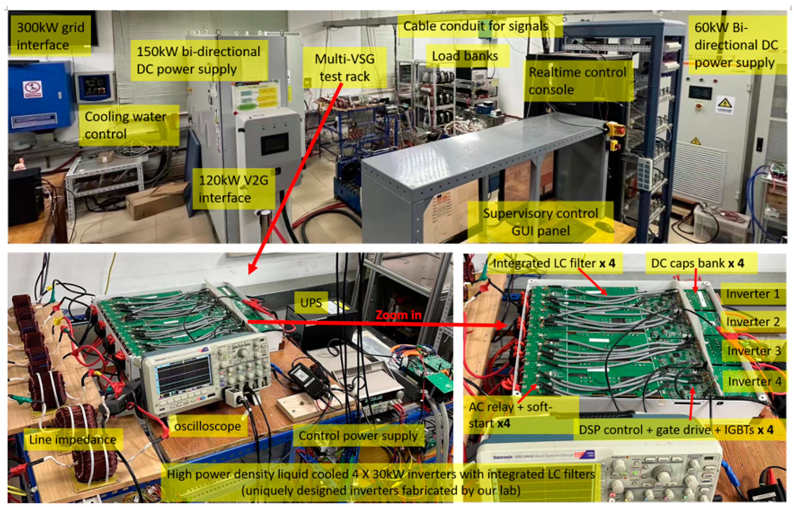
4.1. Experimental Platform

A 30-kVA-rating VSG prototype experimental platform has been developed to validate the proposed decoupling control strategy, with the experimental configuration shown in Figure 11.

The DC side of the VSG prototype is powered by a high-voltage bidirectional programmable DC source. The testbed is constructed to represent a typical low-capacity grid at medium voltages or low voltages, whose line and network impedances are proportionally more resistive compared to high-voltage power systems. Therefore, the grid-connecting line of the VSG prototype was made with an external 1600 μH inductor in series with a 0.5 Ω resistor. The control algorithm is fully implemented on a Texas Instruments TMS320F28335 DSP (Dallas, TX, USA). Voltage and current waveforms are captured using digital oscilloscopes, while power measurements are synchronized to a host computer through CAN communication. The detailed system parameters are presented in Table 1.

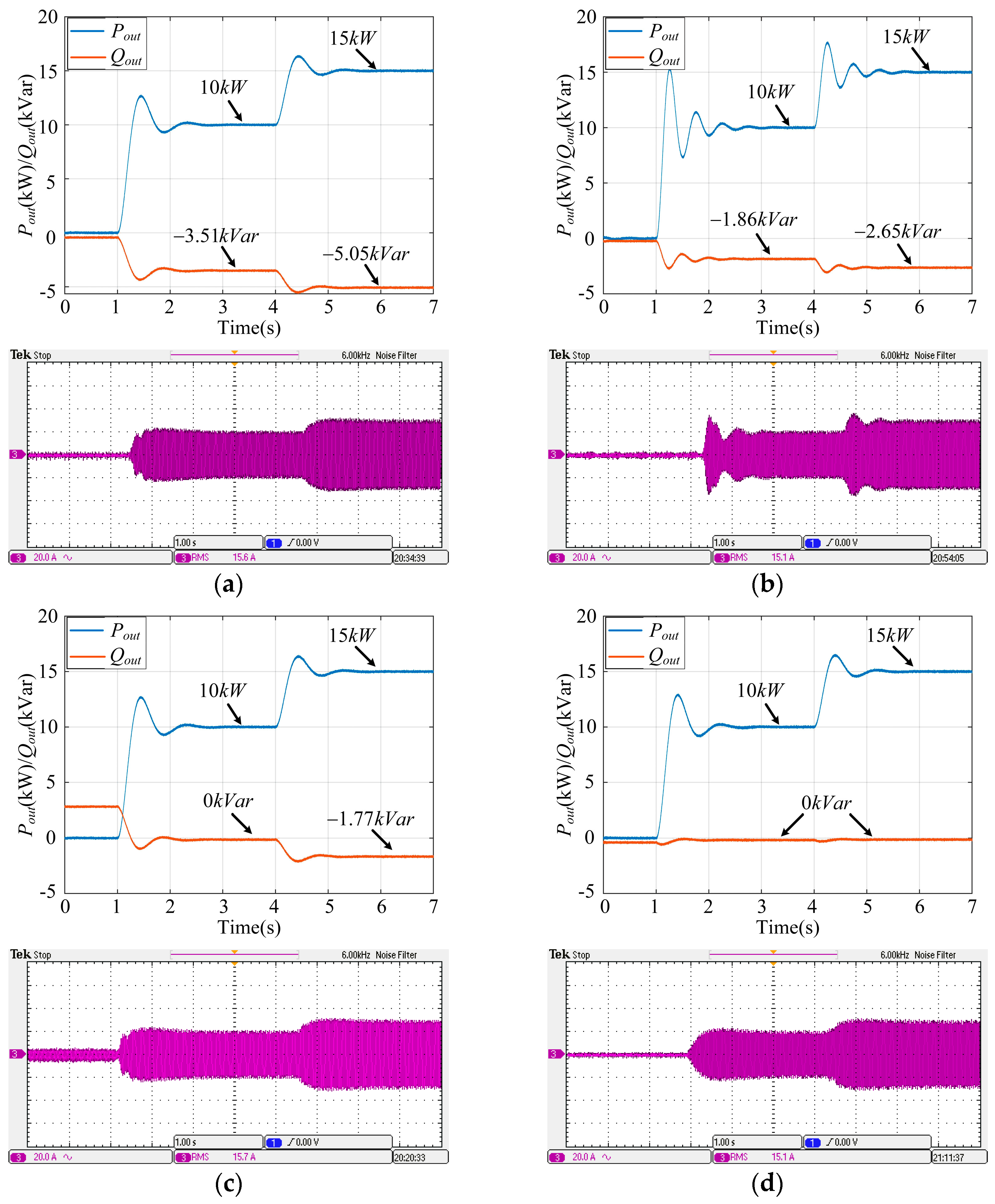
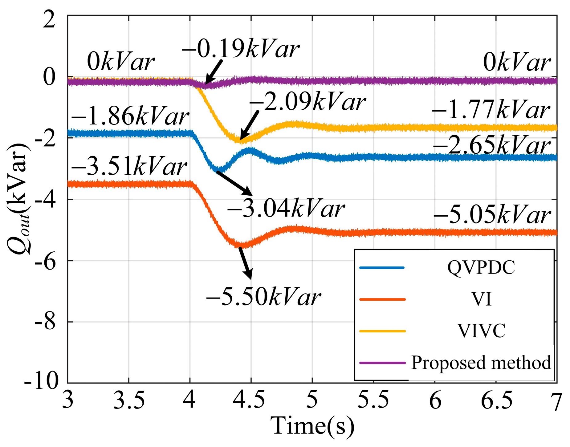
4.2. Experimental Results and Analysis

Figure 12 shows the experimental results of active power output, reactive power output, and output current under four different decoupling methods. The initial active and reactive power references for the VSG are set as P_set = 0 W and Q_set = 0 Var, respectively, at t = 1.0 s. The active power reference is stepped to P_set = 10 kW, followed by a subsequent increase to P_set = 15 kW at t = 4.0 s. The blue traces are the VSG output active powers, and the red traces are the reactive powers.

In Figure 12a, the virtual inductor (VI) method exhibits a steady-state reactive power deviation of 3.51 kVar at a 10 kW active power reference, and then a 5.05 kVar deviation at a 15 kW active power reference. Under this condition, the VSG absorbs significant reactive power from the grid, which not only deteriorates system control accuracy but also leads to system voltage stability issues. The experimental results demonstrate that the VI method has limited power decoupling effectiveness.

Figure 12b illustrates the improved q-axis voltage drop-based power decoupling control (QVPDC) method, which modifies the VI method by employing only q-axis voltage drop compensation. The resulting steady-state reactive power deviation reduces to 1.86 kVar at 10 kW and to 2.65 kVar at 15 kW. While this modification demonstrates a notable improvement in decoupling performance compared to VI methods, complete power decoupling remains unachieved.

Figure 12c shows the experimental results using the virtual inductor and virtual capacitance (VIVC) method, which adds a virtual capacitor to the VI method. The steady-state reactive power deviation measures 0 kVar at 10 kW and 1.77 kVar at 15 kW. These results demonstrate that proper selection of virtual inductor and capacitor parameters can eliminate steady-state power coupling for certain active power operating points. However, this decoupling approach is not adaptive, as evidenced by power deviation with active power reference changes. Furthermore, the method has another limitation, namely exhibiting unintended reactive power output during VSG startup under no-load conditions.

The experimental results of the proposed method are presented in Figure 12d. When the active power reference steps to 10 kW, the reactive power output remains at 0 kVar in a steady state. The subsequent step change in active power reference to 15 kW does not make the reactive power deviate from 0 kVar. The results confirm that the power decoupling of the proposed method is adaptive to varying operating points.

To better evaluate the transient power decoupling effectiveness of the four methods, the reactive power waveforms during the active power step from 10 kW to 15 kW are plotted in the same way as in Figure 13 using the four decoupling methods. Herein, the reactive power transient overshoot values are quantified and labeled in the figure. As the VI, QVPDC, and VIVC methods mainly focus on steady-state power decoupling without considerations for transient power coupling, their reactive power overshoots are obvious during the step change in the VSG active power. The VI, QVPDC, and VIVC methods are −5.5 kVar, −3.04 kVar, and −2.09 kVar, respectively. In the method proposed in this paper, both the steady-state coupling coefficient ξ_tvsg and the transient coupling coefficient ρ₁₁ are used to select virtual impedance values. Therefore, the proposed method maintains zero steady-state reactive power deviation, with negligible transient fluctuations during the power step change.

5. Conclusions

As the existing VSG power decoupling methods are limited in power decoupling performance under varying operating points, this paper proposes a new VSG power decoupling control. By integrating two voltage compensation terms, power decoupling can be achieved for the full operating range. The first voltage compensation term is from adaptively varying virtual resistance and inductance according to operating points. Then, to enhance the power decoupling’s effectiveness in high power ranges, the second voltage compensation term is derived in terms of power angle variation. Finally, the effectiveness of the proposed power decoupling strategy is experimentally validated through comparative lab tests with three existing VSG power decoupling methods.

With the proposed VSG power decoupling methods, the grid-forming and inertia support feature can be achieved for the inverters’ interfacing distributed energy sources without sacrificing the advantages of dynamic and accurate tracking of active and reactive powers with a grid-following inverter. Therefore, this work contributes to the ongoing trend of power electronic grids, increasingly replacing grid-following converters with grid-forming counterparts. In future research, the possibility of unknown line impedance should be considered to make the existing power decoupling methods more adaptable to any grid conditions.

References

1. Zhang, Z.; Zhang, N.; Du, E. Review and Countermeasures on Frequency Security Issues of Power Systems with High Shares of Renewables and Power Electronics. Proc. CSEE 2022, 42, 1–25. [Google Scholar]
2. Cespedes, M.; Sun, J. Impedance Modeling and Analysis of Grid-Connected Voltage-Source Converters. IEEE Trans. Power Electron. 2014, 29, 1254–1261. [Google Scholar] [CrossRef]
3. Zhang, L.; Harnefors, L.; Nee, H. Power-Synchronization Control of Grid-Connected Voltage-Source Converters. IEEE Trans. Power Syst. 2010, 25, 809–820. [Google Scholar] [CrossRef]
4. Liu, J.; Miura, Y.; Ise, T. Comparison of Dynamic Characteristics Between Virtual Synchronous Generator and Droop Control in Inverter-Based Distributed Generators. IEEE Trans. Power Electron. 2016, 31, 3600–3611. [Google Scholar] [CrossRef]
5. Wu, H.; Ruan, X.; Yang, D.; Chen, X.; Zhao, W.; Lv, Z.; Zhong, Q.C. Small-Signal Modeling and Parameters Design for Virtual Synchronous Generators. IEEE Trans. Ind. Electron. 2016, 63, 4292–4303. [Google Scholar] [CrossRef]
6. Meng, X.; Liu, J.; Liu, Z. A Generalized Droop Control for Grid-Supporting Inverter Based on Comparison Between Traditional Droop Control and Virtual Synchronous Generator Control. IEEE Trans. Power Electron. 2019, 34, 5416–5438. [Google Scholar] [CrossRef]
7. Du, J.; Zhao, J.; Zeng, Z.; Mao, L.; Qu, K. Enhanced Power Decoupling Strategy for VSG with Power Control Based on Virtual Power Angle. Proc. CSEE 2024, 44, 8808–8819. [Google Scholar]
8. Li, W.; Kao, C. An Accurate Power Control Strategy for Power-Electronics-Interfaced Distributed Generation Units Operating in a Low-Voltage Multibus Microgrid. IEEE Trans. Power Electron. 2009, 24, 2977–2988. [Google Scholar] [CrossRef]
9. Yan, X.; Zhang, Y. Power coupling analysis of inverters based on relative gain method and decoupling control based on feedforward compensation. In Proceedings of the International Conference on Renewable Power Generation (RPG 2015), Beijing, China, 17–18 October 2015; pp. 1–5. [Google Scholar]
10. Li, B.; Zhou, L.; Yu, X.; Zheng, C.; Liu, J. Improved power decoupling control strategy based on virtual synchronous generator. IET Power Electron. 2017, 10, 462–470. [Google Scholar] [CrossRef]
11. Wen, B.; Boroyevich, D.; Mattavelli, P.; Burgos, R.; Shen, Z. Impedance-based analysis of grid-synchronization stability for three-phase paralleled converters. In Proceedings of the 2014 IEEE Applied Power Electronics Conference and Exposition—APEC, Fort Worth, TX, USA, 16–20 March 2014; pp. 1233–1239. [Google Scholar]
12. Wen, T.; Zou, X.; Guo, X.; Zhu, D.; Peng, L.; Wang, X. Feedforward Compensation Control for Virtual Synchronous Generator to Improve Power Decoupling Capability. In Proceedings of the 14th IEEE Conference on Industrial Electronics and Applications (ICIEA), Xi’an, China, 19–21 June 2019; pp. 2528–2533. [Google Scholar]
13. Zhang, Y.; Raheja, U. An Optimized Virtual Synchronous Generator Control Strategy for Power Decoupling in Grid Connected Inverters. In Proceedings of the 2019 IEEE Energy Conversion Congress and Exposition (ECCE), Baltimore, MD, USA, 29 September–3 October 2019; pp. 49–54. [Google Scholar]
14. Jia, W.; Xu, Z.; Gerada, C. Dynamic power decoupling for low-voltage ride-through of grid-forming inverters. IEEE Trans. Power Electron. 2022, 37, 3878–3891. [Google Scholar] [CrossRef]
15. Wang, Y.; Wai, R. Adaptive Fuzzy-Neural-Network Power Decoupling Strategy for Virtual Synchronous Generator in Micro-Grid. IEEE Trans. Power Electron. 2022, 37, 3878–3891. [Google Scholar]
16. Wang, Z.; Wang, Y.; Davari, M.; Blaabjerg, F. An Effective PQ-Decoupling Control Scheme Using Adaptive Dynamic Programming Approach to Reducing Oscillations of Virtual Synchronous Generators for Grid Connection with Different Impedance Types. IEEE Trans. Ind. Electron. 2024, 71, 3763–3775. [Google Scholar]
17. Yang, Y.; Xu, J.; Li, C. A New Virtual Inductance Control Method for Frequency Stabilization of Grid-Forming Virtual Synchronous Generators. IEEE Trans. Ind. Electron. 2023, 90, 441–451. [Google Scholar]
18. Guerrero, J.; Matas, J.; De Vicuna, L.; Castilla, M.; Miret, J. Decentralized control for parallel operation of distributed generation inverters using resistive output impedance. IEEE Trans. Ind. Electron. 2007, 54, 994–1004. [Google Scholar] [CrossRef]
19. Vandoorn, T.; Meersman, B.; Kooning, J.; Vandevelde, L. Directly-coupled synchronous generators with converter behavior in islanded microgrids. IEEE Trans. Power Syst. 2012, 27, 1395–1406. [Google Scholar]
20. Guerrero, J.; De Vicuna, L.; Matas, J.; Castilla, M.; Miret, J.; de Vicuna, L.G. Output impedance design of parallel-connected ups inverters with wireless load-sharing control. IEEE Trans. Ind. Electron. 2005, 52, 1126–1135. [Google Scholar] [CrossRef]
21. Wen, T.; Zhu, D.; Zou, X.; Jiang, B.; Peng, L.; Kang, Y. Power Coupling Mechanism Analysis and Improved Decoupling Control for Virtual Synchronous Generator. IEEE Trans. Power Electron. 2021, 36, 3028–3041. [Google Scholar] [CrossRef]
22. Yan, X.; Cui, S.; Jia, J. Virtual steady state synchronous negative impedance of a VSG power decoupling strategy. Power Syst. Prot. Control 2020, 48, 102–113. [Google Scholar]
23. Li, M.; Wand, Y.; Liu, Y. Enhanced power decoupling strategy for virtual synchronous generator. IEEE Access 2020, 8, 73601–73613. [Google Scholar]
24. Hu, Y.; Shao, Y.; Yang, R.; Long, X. A Configurable Virtual Impedance Method for Grid-Connected Virtual Synchronous Generator to Improve the Quality of Output Current. IEEE J. Emerg. Sel. Top. Power Electron. 2020, 8, 2404–2419. [Google Scholar] [CrossRef]
25. Long, B.; Zhu, S.; Rodriguez, J.; Chong, K.T. Enhancement of Power Decoupling for Virtual Synchronous Generator: A Virtual Inductor and Virtual Capacitor Approach. IEEE Trans. Ind. Electron. 2023, 70, 6830–6843. [Google Scholar]
Figure 1. VSG control block diagram.
Energies 18 01878 g001
Figure 2. VSG equivalent circuit diagram.
Energies 18 01878 g002
Figure 3. (a) ξvsg with varying line resistor; (b) ρ11 with varying line resistor; (c) simulation of VSG output powers.
Energies 18 01878 g003
Figure 4. The first voltage compensation term from virtual resistance and inductance.
Energies 18 01878 g004
Figure 9. The overall block diagram of the proposed decoupling control.
Energies 18 01878 g009
Figure 10. Change in ξtvsg with line impedance angle θzt and power angle θ.
Energies 18 01878 g010
Figure 5. Trends of ξtvsg with the additional virtual resistor and virtual inductor.
Energies 18 01878 g005
Figure 6. Trends of ρ11 with the additional virtual resistor and virtual inductor.
Energies 18 01878 g006
Figure 7. The virtual resistor and virtual inductor online adjustment calculation process.
Energies 18 01878 g007
Figure 8. Change in ξtvsg with total equivalent impedance angle θzt and power angle θ.
Energies 18 01878 g008
Figure 11. Experimental configuration of VSG.
Energies 18 01878 g011
Figure 12. The effectiveness of four VSG decoupling methods: (a) VI method; (b) QVPDC method; (c) VIVC method; (d) proposed method.
Energies 18 01878 g012
Figure 13. Transient power decoupling effectiveness of the four methods.
Energies 18 01878 g013