Fast Monocular Measurement via Deep Learning-Based Object Detection for Real-Time Gas-Insulated Transmission Line Deformation Monitoring

Abstract

Deformation monitoring of Gas-Insulated Transmission Lines (GILs) is critical for the early detection of structural issues and for ensuring safe power transmission. In this study, we introduce a rapid monocular measurement method that leverages deep learning for real-time monitoring. A YOLOv10 model is developed for automatically identifying regions of interest (ROIs) that may exhibit deformations. Within these ROIs, grayscale data is used to dynamically set thresholds for FAST corner detection, while the Shi–Tomasi algorithm filters redundant corners to extract unique feature points for precise tracking. Subsequent subpixel refinement further enhances measurement accuracy. To correct image tilt, ArUco markers are employed for geometric correction and to compute a scaling factor based on their known edge lengths, thereby reducing errors caused by non-perpendicular camera angles. Simulated experiments validate our approach, demonstrating that combining refined ArUco marker coordinates with manually annotated features significantly improves detection accuracy. Our method achieves a mean absolute error of no more than 1.337 mm and a processing speed of approximately 0.024 s per frame, meeting the precision and efficiency requirements for GIL deformation monitoring. This integrated approach offers a robust solution for long-term, real-time monitoring of GIL deformations, with promising potential for practical applications in power transmission systems.

1. Introduction

Gas-Insulated Transmission Lines (GILs) are high-voltage, high-current power transmission systems that utilize SF₆ gas or SF₆/N₂ gas mixtures for insulation, with conductors and outer casings arranged coaxially. Compared to conventional overhead and cable transmission lines, GILs offer advantages such as higher transmission capacity, reduced transmission losses, environmental friendliness, and versatility in application, which have facilitated their widespread global adoption [1,2,3]. Deformation data on GIL pipelines under operational loads serve as critical indicators for assessing structural health and preventing structural failures. Therefore, developing effective deformation monitoring methods for GIL pipelines is of paramount engineering significance for ensuring the safe and reliable operation of both GIL systems and the broader power transmission infrastructure.

Traditional deformation monitoring methods for GILs involve direct mechanical contact of sensitive measurement components, such as resistive strain gauges and fiber optic sensors, with the surface of the target structure to acquire deformation data at specific points. However, these approaches are characterized by low measurement efficiency, vulnerability to strong electromagnetic interference, and high implementation complexity. Consequently, they are inadequate for large-scale and long-term deformation monitoring applications [4,5,6].

Recent advancements in computer hardware and image processing technologies have facilitated the gradual integration of machine vision into structural displacement monitoring for power transmission lines [7]. Yang et al. [8] utilized monocular vision technology to extract the contours of transmission towers and accurately measure their degree of inclination. Wang et al. [9] developed a sag variation monitoring method for transmission lines under icing conditions utilizing binocular vision. Zhang et al. [10] introduced a Region of Interest (ROI) key point method based on the geometric configuration of transmission towers to obtain displacement information of tower structures. Li et al. [11] combined deep learning approaches to propose a real-time safety clearance monitoring method for transmission corridors. Fauzan et al. [12] proposed a rapid method for measuring GIL deformation that achieves a mean absolute error of less than 3 mm. In their approach, artificial targets affixed to the surface of the GIL facility serve as monitoring points, with the displacement of these targets indicating the extent of deformation. However, since the pixel coordinates of these targets are obtained through a semi-manual process and the measurements are conducted offline, the procedure is relatively complex and labor-intensive. Future studies should focus on enhancing detection efficiency and automation while maintaining the required accuracy, thereby reducing both measurement complexity and personnel involvement.

Fundamentally, the studies mentioned above primarily focused on employing machine vision for displacement detection or monitoring in power transmission line structures. However, research on machine vision-based deformation monitoring methods for GIL pipelines remains in its nascent stages. Determining the pixel coordinates of markers in an image can be framed as an object detection problem. Among traditional detection methods, template matching has long been recognized as an effective approach. Xu et al. [13] applied monocular vision techniques for multi-point displacement measurements on bridges. By estimating camera parameters from point pairs with known coordinates and tracking bridge feature points through template matching, they achieved millimeter-level precision in capturing bridge vibrations. Similarly, Brownjohn et al. [14] converted displacement data at bridge measurement points by using the distance between the camera’s optical center and the measurement plane (i.e., line features), also employing template matching for target tracking and identification. Yang et al. [15] further improved target localization in complex backgrounds by introducing a dynamic template updating strategy.

While template matching effectively extracts targets, its application in GIL deformation monitoring, which requires multiple manual markers, introduces additional complexity in determining marker positions. Moreover, template matching is relatively slow and computationally demanding, as it relies on pre-prepared template images. During target motion, factors such as noise, illumination fluctuations, and background variations may cause mismatches, thereby necessitating increased manual intervention. A rapid method for rough localization of the target region could substantially accelerate both detection and tracking. In recent years, the deep learning-based YOLO algorithm has demonstrated high adaptability and detection efficiency across diverse scenarios, satisfying the requirements of such applications. Wu et al. [16] analyzed object detection algorithms in traditional remote sensing imagery and noted that template matching shows limited robustness under conditions of rotation or scaling. They subsequently refined the YOLOv8 framework to improve detection accuracy for multi-scale objects and small targets. Li et al. [17] combined the YOLO-T algorithm with manual marking and monocular vision-based localization to enable underwater robots to detect and locate targets. Yang et al. [18] applied an improved YOLOv3 model for the coarse localization of tea bud pixel coordinates by using the two coordinate points provided by the detection bounding box to identify the region of interest, extracting it as a sub-image and applying subsequent image processing techniques for precise localization.

The YOLO detection model allows rapid coarse localization of manual markers, significantly enhancing both detection speed and accuracy—even achieving real-time performance. These markers yield robust corner features that serve as reliable tracking targets. Consequently, after extracting the sub-image containing a marker, further extraction of corner features facilitates subsequent tracking and measurement. For instance, the classical Oriented FAST and Rotated BRIEF (ORB) [19] algorithm uses the Features from Accelerated Segment Test (FAST) to extract corner features, making it widely applicable in scenarios that prioritize real-time performance over ultra-high precision. However, the conventional FAST algorithm is constrained by its reliance on manually specified thresholds, which may not be optimal for detecting corners across an entire image, thus reducing detection accuracy. To address this limitation, Li et al. [20] optimized the pixel comparison order using decision trees and applied non-maximum suppression to filter feature points, thereby enhancing detection performance.

The proposed research approach involves first performing rapid coarse localization of the marker region and extracting it as a sub-image, followed by the extraction of corner features for tracking. This method not only enables real-time localization but also supports automatic tracking of corner points. In monocular measurement, the calculation of the actual displacement of a target is often performed using methods such as the proportional factor approach. This technique involves converting the physical displacement by leveraging known parameters, such as the distance between the measurement point and the target or identifiable texture features present on the target itself [21,22]. These techniques convert physical displacements by utilizing the known distance between measurement points and the target or by leveraging known texture features on the target surface. However, both methods are adversely affected by the misalignment between the camera optical axis and the measurement plane, which can significantly impact measurement accuracy. Research conducted under laboratory conditions, as reported in reference [22], indicates that the proportional factor method is particularly sensitive to the angle between the camera’s optical axis and the target plane. It is recommended that this angle be maintained within 10°, and the distance from the camera to the target should not exceed 3.7 m to minimize measurement errors. To address the limitations imposed by the camera’s placement angle, image tilt correction is performed to align the image with an ideal imaging plane that is perpendicular to the optical axis. Nevertheless, a significant limitation of monocular measurements is their inability to capture out-of-plane displacements, which restricts the camera’s measurement pose. Instead of constraining the camera’s pose during monitoring, image correction techniques can address this issue. For example, Shan et al. [23] employed prior instrument information to correct perspective distortions, thereby improving the accuracy of their automatic meter reading algorithm. Consequently, when measuring marker displacements using monocular vision, incorporating image tilt correction techniques supported by prior information warrants further investigation and validation.

Issues such as the compatibility between GIL pipeline deformation characteristics and machine vision techniques, as well as the real-time automation of the monitoring process, remain areas that require further exploration. To address the limitations of traditional deformation monitoring methods for GIL, we propose an automatic, real-time monocular measurement approach tailored to the specific deformation characteristics of GIL pipelines. Experimental validation demonstrates the accuracy, timeliness, and robustness of the proposed method, thereby providing a feasible and effective monitoring solution for GIL pipeline deformations. Compared to previous studies, our proposed method reduces measurement complexity and costs while significantly accelerating deformation monitoring, achieving real-time performance without compromising accuracy. Furthermore, by integrating the Shi–Tomasi algorithm with adaptive threshold computation, our approach eliminates the need for manual intervention and enhances the detection precision of the traditional FAST algorithm for automatic extraction and tracking of marker features. Finally, by leveraging the physical information provided by ArUco codes, we implement image tilt correction to eliminate additional errors caused by non-perpendicular alignment between the camera’s optical axis and the measurement plane in monocular setups.

2. Design of a Monocular Measurement System for GIL Deformation

Due to the highly repetitive texture features on the surfaces of GIL pipeline components, texture-based feature extraction and matching methods, such as Scale-Invariant Feature Transform (SIFT) [24], Speeded-Up Robust Features (SURF) [25], and Oriented FAST and Rotated BRIEF (ORB) [26], often result in repetitive local feature matches. This repetition impedes tracking algorithms from accurately identifying and following individual feature points. Implementing artificial markers effectively addresses this issue by simplifying the measurement process, transforming GIL pipeline deformation monitoring into the calculation of displacements for unique feature points within the markers. Additionally, spraying markers onto the pipeline surface is preferable to affixing them directly, as it prevents positional shifts of the markers caused by pipeline deformation.

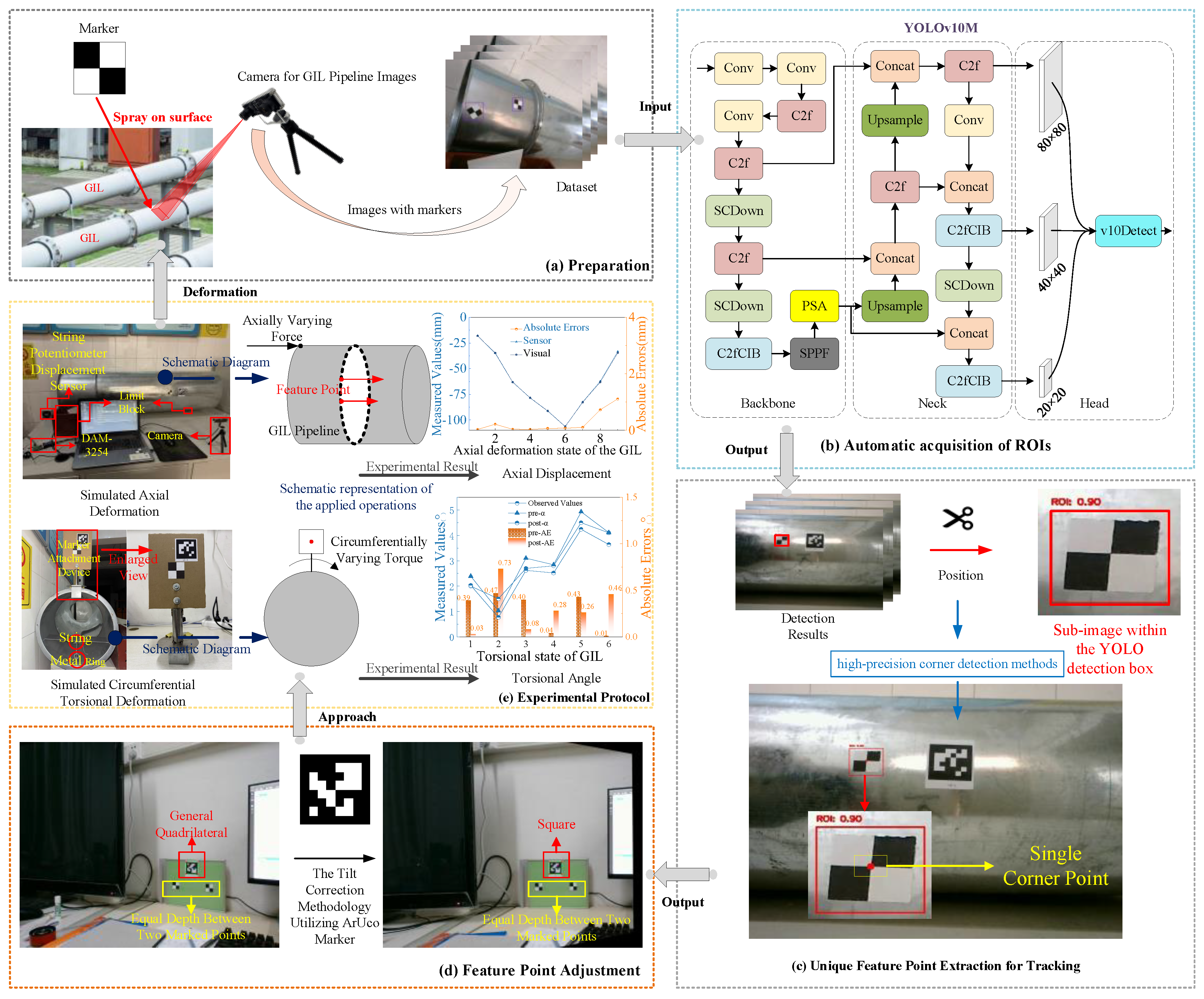
A monocular measurement method is employed to monitor GIL pipeline deformations, with the specific technical approach illustrated in Figure 1. The monitoring system’s hardware includes artificial markers, ArUco markers, a computer, and a camera, while the software algorithms are developed using Python 3.8 and Pytorch 2.0.0 deep learning platforms. For practical operational convenience, printed artificial markers are used during the monitoring process. The effectiveness of the proposed method is validated through displacement and twist angle measurements of a feature point on the GIL pipeline surface, demonstrating its feasibility for accurate and real-time deformation monitoring.

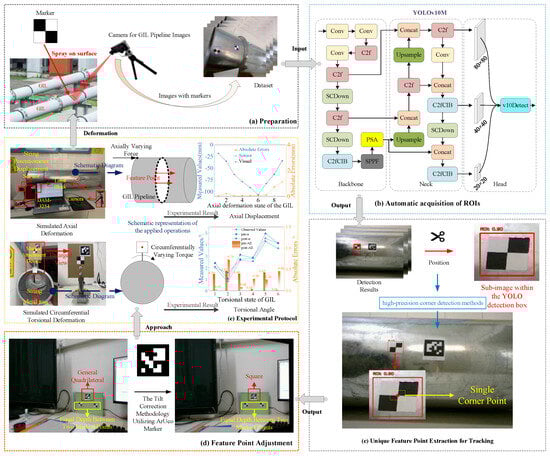
Figure 1. A real-time monitoring method for GIL deformation: overview and pipeline using YOLOv10 object detection and sub-pixel corner detection.

Initially, images containing markers are collected to create a dataset for training the YOLOv10 model. This enables the rapid and automatic localization of markers within the entire image, providing their positional information. Subsequently, sub-images, each containing a single marker, are extracted and processed to identify the coordinates of the target corner point within each marker that requires tracking. To address the loss of depth information inherent in monocular measurements, the known physical edge length of the ArUco marker is utilized. Additionally, the coordinates of the four corners of the ArUco marker are employed to calculate the projection transformation matrix, which is applied to correct image tilt and reduce measurement errors caused by the lack of perpendicularity between the camera’s optical axis and the imaging plane. Finally, by integrating the positional information of the marker detected by the YOLO model, the coordinates of the target corner point in the marker within the cropped sub-image, the known physical dimensions of the ArUco marker, and the perspective transformation matrix, the actual displacement of each corner point relative to the reference position can be calculated.

3. Related Methods and Modeling Procedures

3.1. Region of Interest Extraction

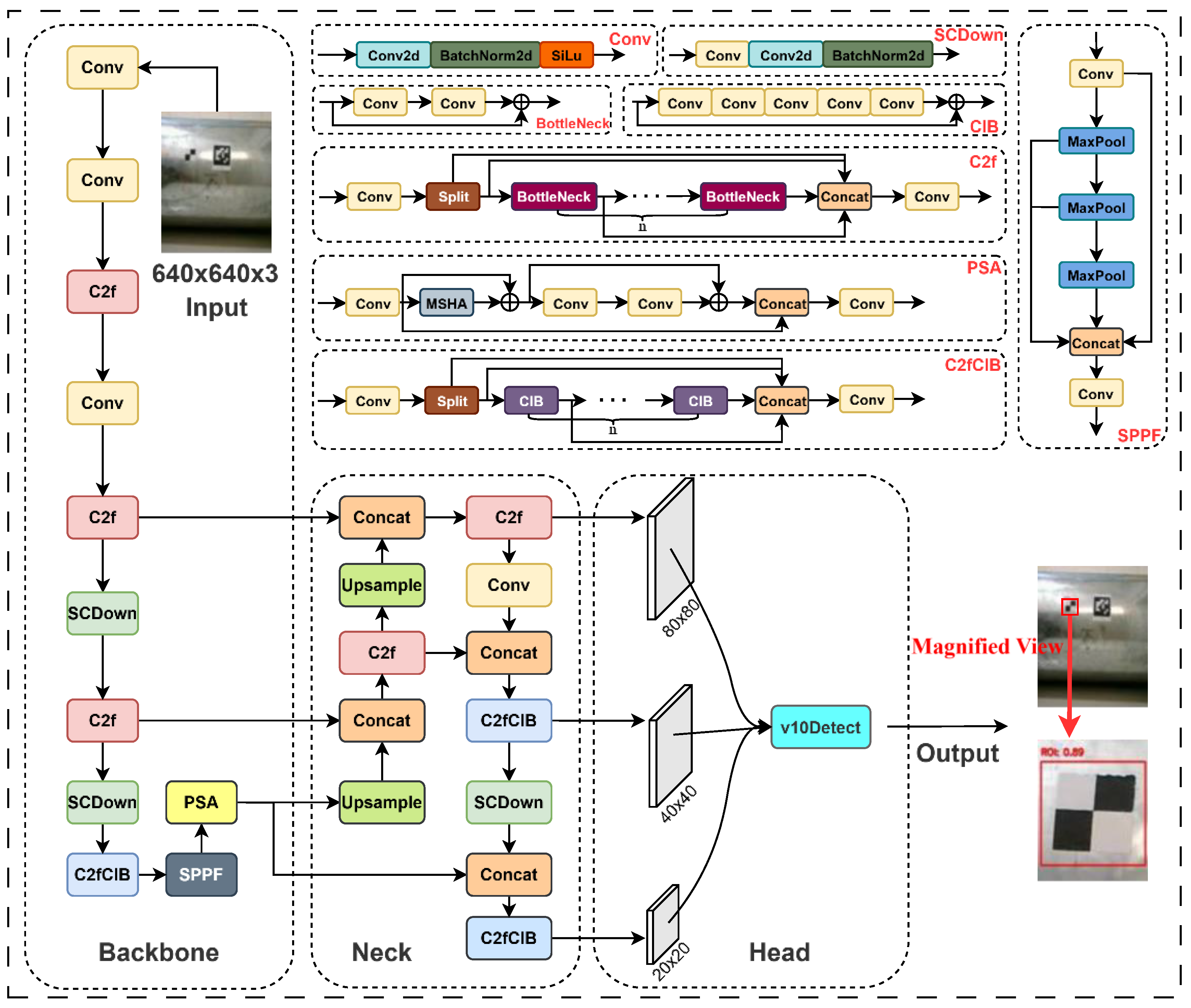
Considering that the YOLOv10 [27] model combines high performance with high efficiency, it provides an option for end-to-end target detection. Consequently, YOLOv10 was selected as the deep learning model for extracting regions of interest (ROIs) in this study, as shown in Figure 2. The YOLOv10 framework offers six variants—N, S, M, B, L, and X—each progressively increasing in model size, accuracy, and inference latency. This range allows for the selection of an appropriate model variant based on the specific requirements of size and computational efficiency for ROI extraction tasks.

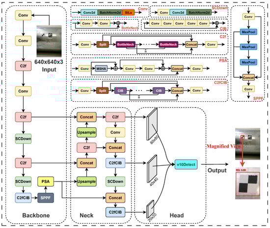
Figure 2. A YOLOv10 model architecture.

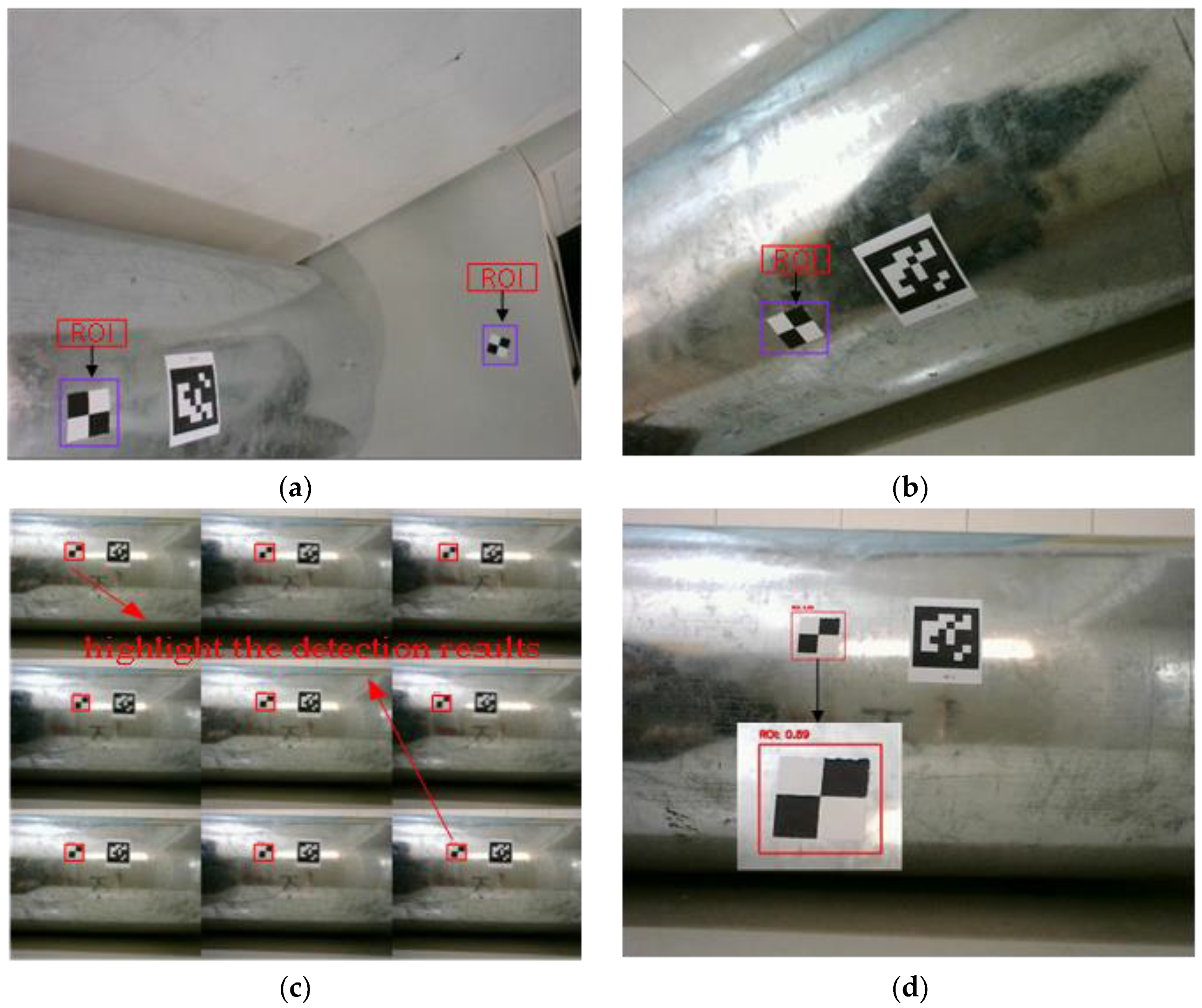
In this study, images of GILs were captured under various measurements and environmental conditions. A subset of these images was randomly selected for data augmentation, ultimately expanding the dataset to 930 images. Using the Roboflow platform, markers within the images were annotated with bounding rectangles, as illustrated in Figure 3a,b. During the annotation process, bounding boxes were drawn to delineate the regions containing the markers, ensuring that each marker was fully encompassed while minimizing irrelevant background. After manual annotation, all annotations were meticulously verified to maximize both consistency and accuracy. The dataset was then divided into training, validation, and testing sets in an 8:1:1 ratio. A YOLOv10M model, depicted in Figure 2, was constructed and trained on the training set to achieve the automatic and rapid extraction of marked regions within the images. The deployment, training, and inference of the model were conducted on a remote GPU setup, featuring an NVIDIA RTX 3090 with 24 GB of memory and an eight-core CPU, with the number of training epochs set to 500. The trained model yielded detection results as shown in Figure 3c,d, enabling the extraction of sub-images containing the markers and their positional information.

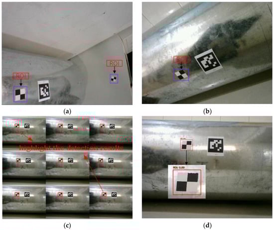
Figure 3. Illustration of ROI extraction. (a) Example #1 of annotation status. (b) Example #2 of annotation status. (c) Marker extraction status. (d) Marker extraction details.

3.2. Feature Point Extraction Within ROI

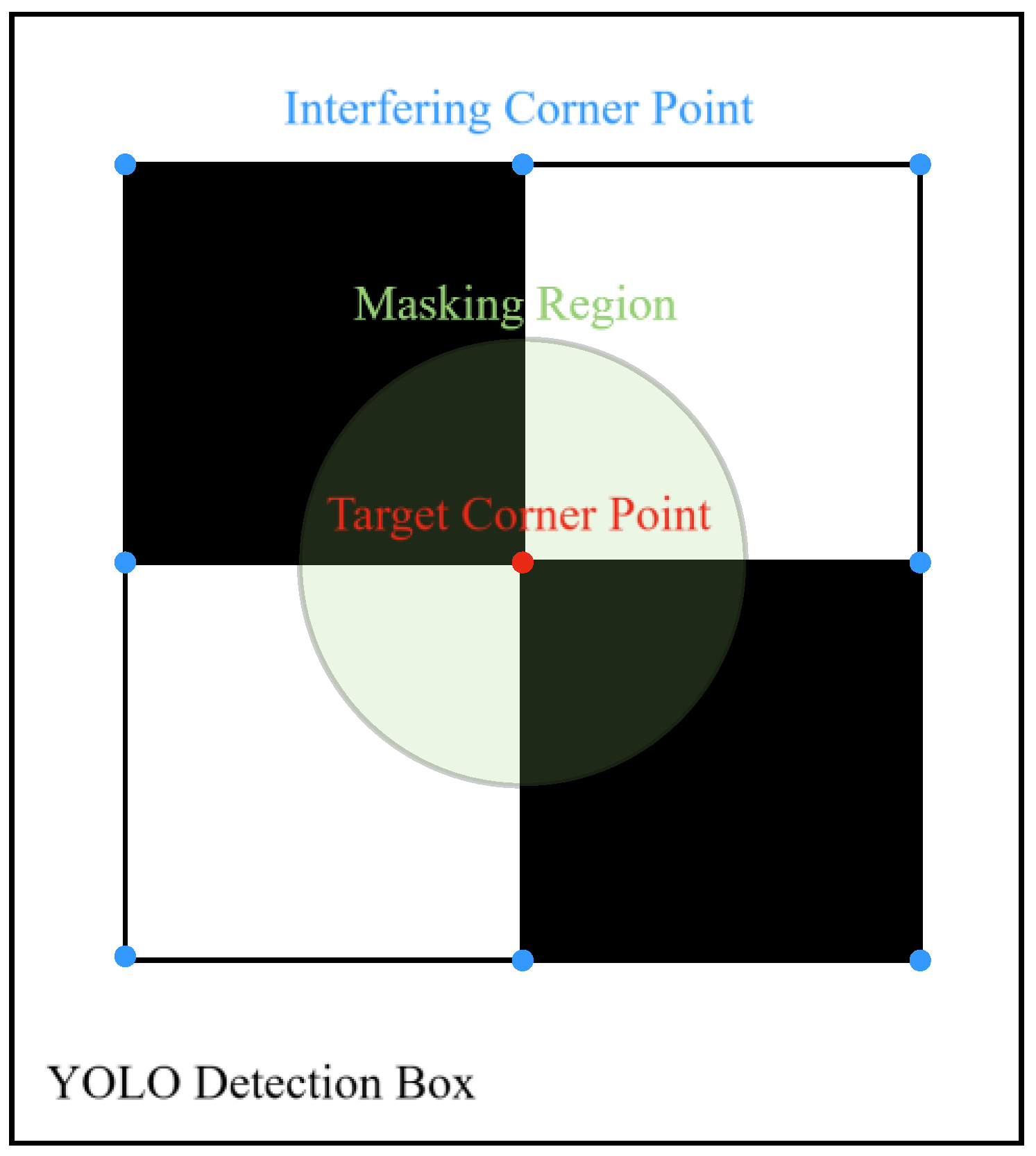
After extracting the sub-image containing the marker region (as shown in Figure 3d), it is essential to identify the central corner point within the marker, referred to as the “target corner point”. This point is uniquely defined for each marker and serves as the focal point for subsequent displacement measurements. The precise location of the target corner point is illustrated in Figure 4. By tracking the displacement of this target corner point, we can effectively quantify the deformation of the GIL at specific locations. However, corner points located at the edges of the marker may compromise the uniqueness of the detection result. To enhance the automation of the monitoring system, it is necessary to restrict the region for corner point detection. Firstly, the central pixel point (O_P) of the YOLO detection bounding box is identified. Next, the length of the shortest side of the bounding rectangle is measured, and one-quarter of this length is designated as R. Finally, a masked region is created with O_P as the center and R as the pixel radius, as illustrated in Figure 4. The subsequent corner detection algorithm is executed within this constrained masked region.

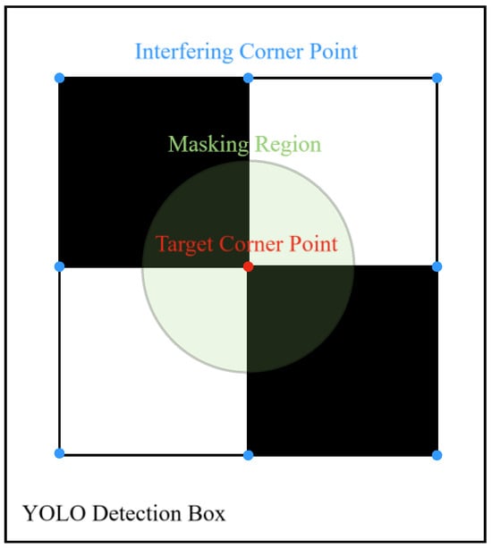
Figure 4. Mask Schematic.

Although the traditional Features from Accelerated Segment Test (FAST) algorithm offers rapid detection speeds [28,29], it relies on empirically set thresholds to achieve optimal detection results and is prone to false positives, which impede the implementation of subsequent measurement procedures. To accurately extract the target corner point in the mark, a high-precision corner detection method with region-adaptive thresholds is proposed. The specific detection steps are as follows.

3.2.1. Region-Adaptive Threshold Calculation

The mean grayscale value of an image represents its overall brightness level, while the standard deviation of grayscale values indicates the degree of dispersion within the image. Utilizing Equation (3) for automatic threshold calculation allows the threshold to adapt dynamically to variations in image brightness and contrast, thereby enhancing both flexibility and robustness.

Assuming that the image within the YOLO detection bounding box has dimensions m × n, where each pixel’s grayscale value is denoted as I (i, j), the mean grayscale value μ for this region is given by:

$$\mu ={\displaystyle \frac{1}{mn}}{\displaystyle \sum _{i=1}^m{\displaystyle \sum _{j=1}^{n}I\left(i,j\right)}}$$

(1)

The standard deviation of the grayscale value, denoted as σ, is calculated as follows:

$$\sigma =\sqrt{{\displaystyle \frac{1}{mn}}{\displaystyle \sum _{i=1}^m{\displaystyle \sum _{j=1}^n{\left(I\left(i,j\right)-\mu \right)}^2}}}$$

(2)

The formula for the detection threshold T is as follows:

$$T=\mu -\sigma$$

(3)

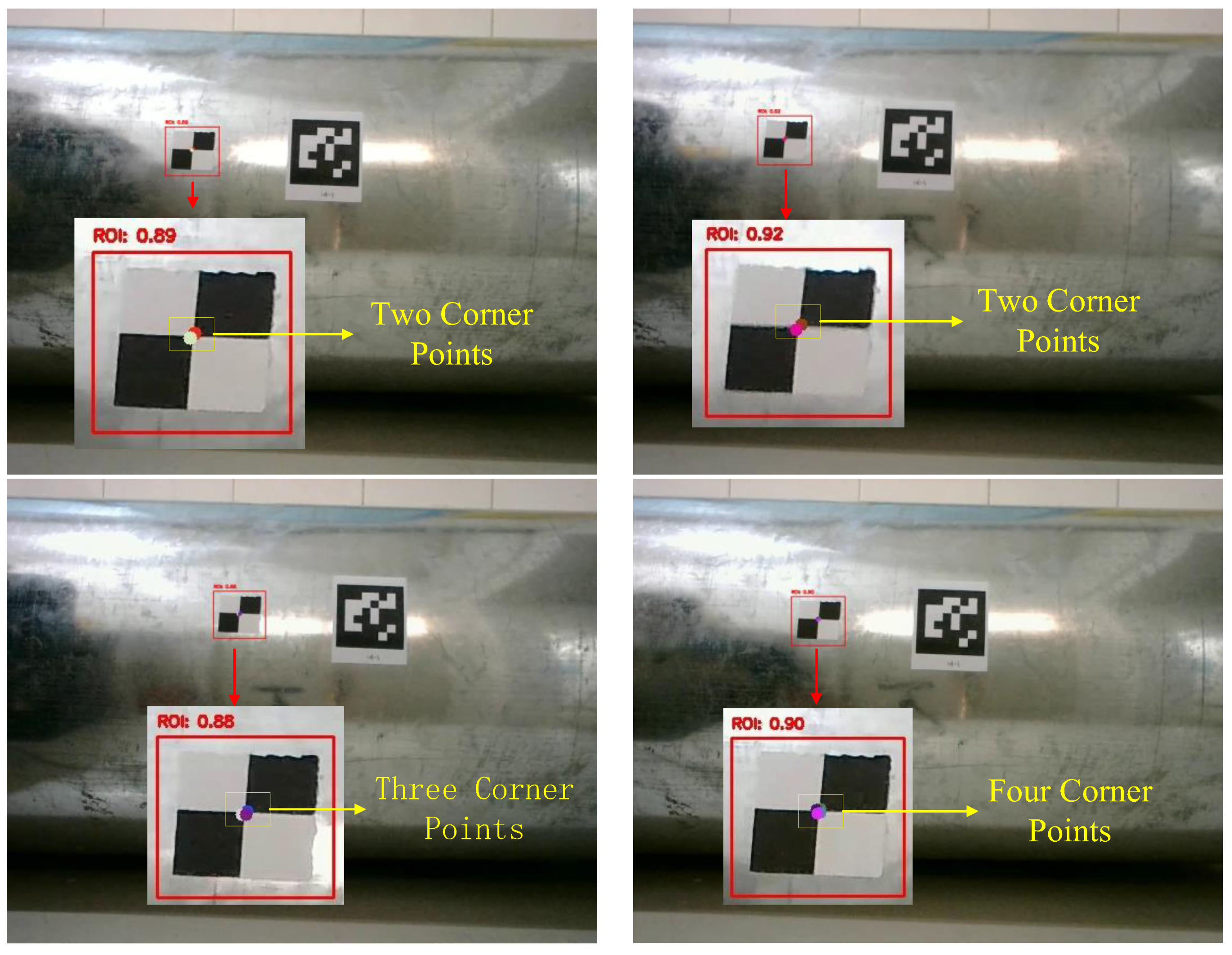
The corner detection results obtained using the FAST algorithm with adaptive thresholding are illustrated in Figure 5.

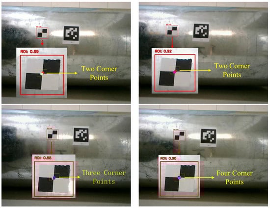
Figure 5. Preliminary improved corner point detection results.

3.2.2. Elimination of Redundant Corner Points

In the detection results presented in Figure 5, redundant corner points do not meet the specified requirements. Consequently, it is necessary to refine the detected corner points further. Compared to the FAST algorithm, the Shi–Tomasi algorithm, based on image gradients, offers higher detection precision. However, it entails greater computational complexity and longer processing times [30]. To balance efficiency and accuracy, we treat the corner points detected by FAST as candidate points and subsequently apply the Shi–Tomasi algorithm for precise detection. This two-step approach effectively suppresses false corner points, thereby ensuring the uniqueness and reliability of the detection results.

The Shi–Tomasi corner detection algorithm determines whether a current pixel constitutes a corner by calculating the variation in grayscale values within a sliding window. The energy function, E (x, y), represents the local grayscale variation of windows and is calculated as follows:

$$E\left(x,y\right)={\displaystyle \sum _{u,v}w\left(u,v\right){\left[I\left(u+x,v+y\right)-I\left(u,v\right)\right]}^2}$$

(4)

where (u, v) represents the pixel coordinates; I (u, v) represents the pixel grayscale of the coordinate point, x, and y denotes the displacements within the window; I (u + x, v + y) represents the grayscale of the pixel at this new position; and w (u, v) signifies the weighting function. By expanding I (u + x, v + y) as a binary function, E (x, y) can be expressed as follows:

$$E\left(x,y\right)=\left[\begin{array}{cc}x& y\end{array}\right]\left[w\left(u,v\right){\displaystyle \sum _{u,v}\left[\begin{array}{cc}{I}_u^2& I_u{I}_v\\ I_u{I}_v& I_v^2\end{array}\right]}\right]\left[\begin{array}{c}x\\ y\end{array}\right]$$

(5)

where I_u and I_v denote the image gradients in the respective horizontal and vertical directions. Let M₀ represent the matrix in E (x, y):

$${\mathit{M}}_0=w\left(u,v\right){\displaystyle \sum _{u,v}\left[\begin{array}{cc}{I}_u^2& I_u{I}_v\\ I_u{I}_v& I_v^2\end{array}\right]}$$

(6)

Therefore, the corner point response function R (u, v) at coordinates (u, v) can be calculated as follows:

$$R\left(u,v\right)=\min \left({\lambda }_1,{\lambda }_2\right)$$

(7)

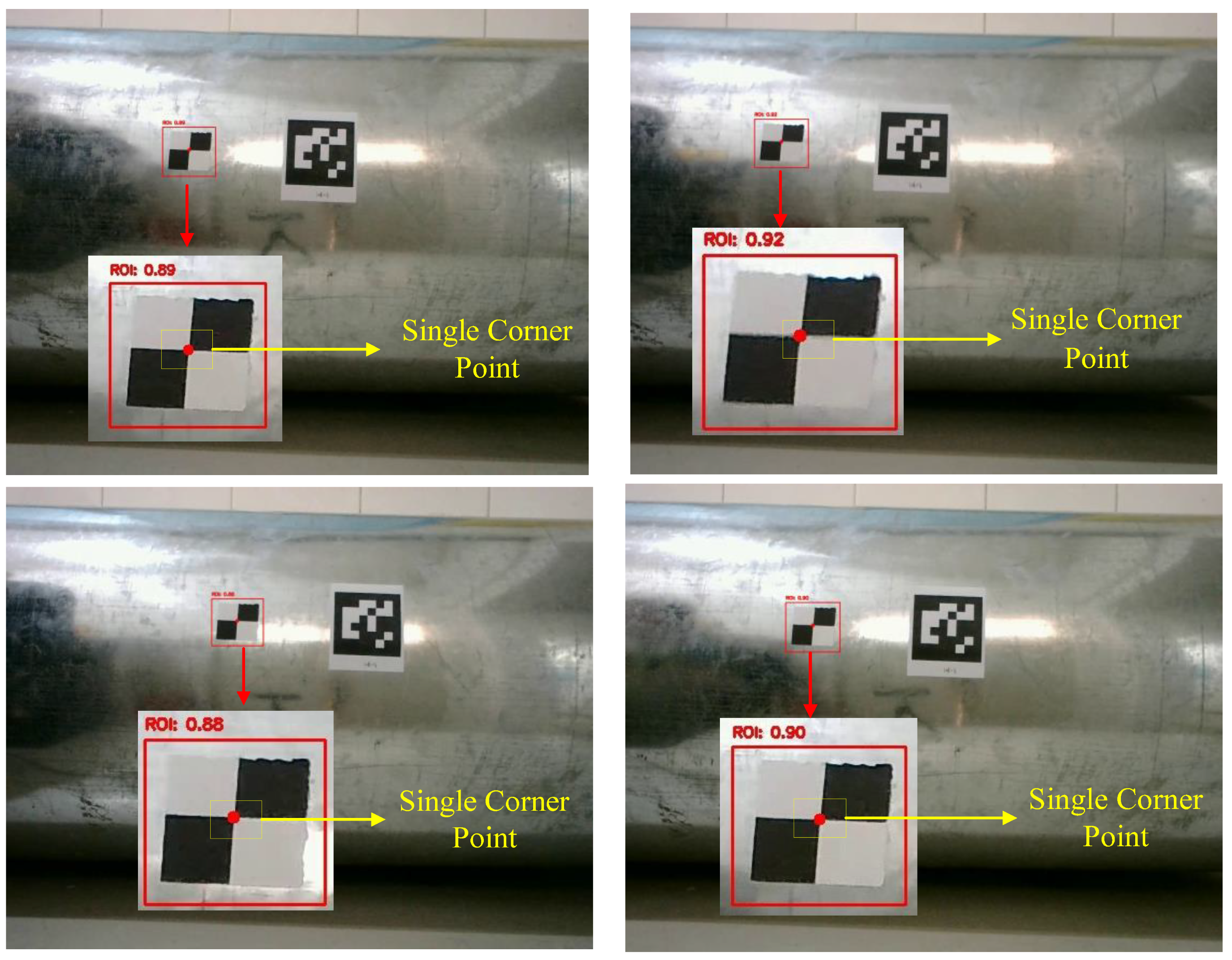
where λ₁ and λ₂ are the eigenvalues of the second moment matrix M₀. As illustrated in Figure 5, corner point filtering is performed within the detection frame using the Shi–Tomasi corner detection algorithm. The results, shown in Figure 6, highlight the effectiveness of the algorithm in accurately isolating distinctive corners, specifically the target corner point that is uniquely present in each marker.

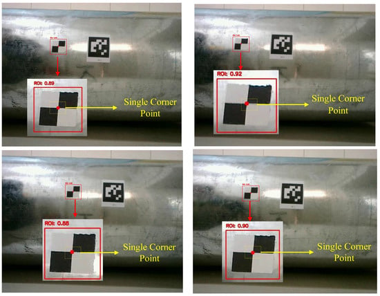
Figure 6. Results of corner point selection.

3.2.3. Subpixel Refinement of Corner Point Coordinates

After removing redundant corner points, we obtained the pixel polar coordinates of the target corner point in the marker. However, in certain application scenarios where higher precision is required, subpixel-level corner coordinates are necessary [31,32]. Therefore, this study performs subpixel repositioning of the detected corner coordinates to extract more accurate corner information and conducts comparative analyses of the results in subsequent experiments.

The grayscale intensity I (x, y) of a pixel at coordinates (x, y) can be approximated using the following quadratic function:

$$I\left(x,y\right)=a+bx+cy+d{x}^2+e{y}^2+fxy$$

(8)

Here, a, b, c, d, and e are unknown coefficients. To determine these coefficients, we construct an objective function, E_p (x, y), which measures the difference between the actual grayscale value I_{x, y} at pixel (x, y) within a window of size W and the fitted grayscale value I (x, y) obtained from the quadratic approximation. By minimizing E_p (x, y), we can estimate the unknown coefficients in Equation (8). Subsequently, the subpixel coordinates of the corner point are identified by locating the extrema of I (x, y). The objective function E_p (x, y) is calculated as follows:

$$E_p\left(x,y\right)={\displaystyle \sum _{x,y\in W}{\left[I_{x,y}-I\left(x,y\right)\right]}^2}$$

(9)

3.3. Image Tilt Correction and Scaling Factor Calculation

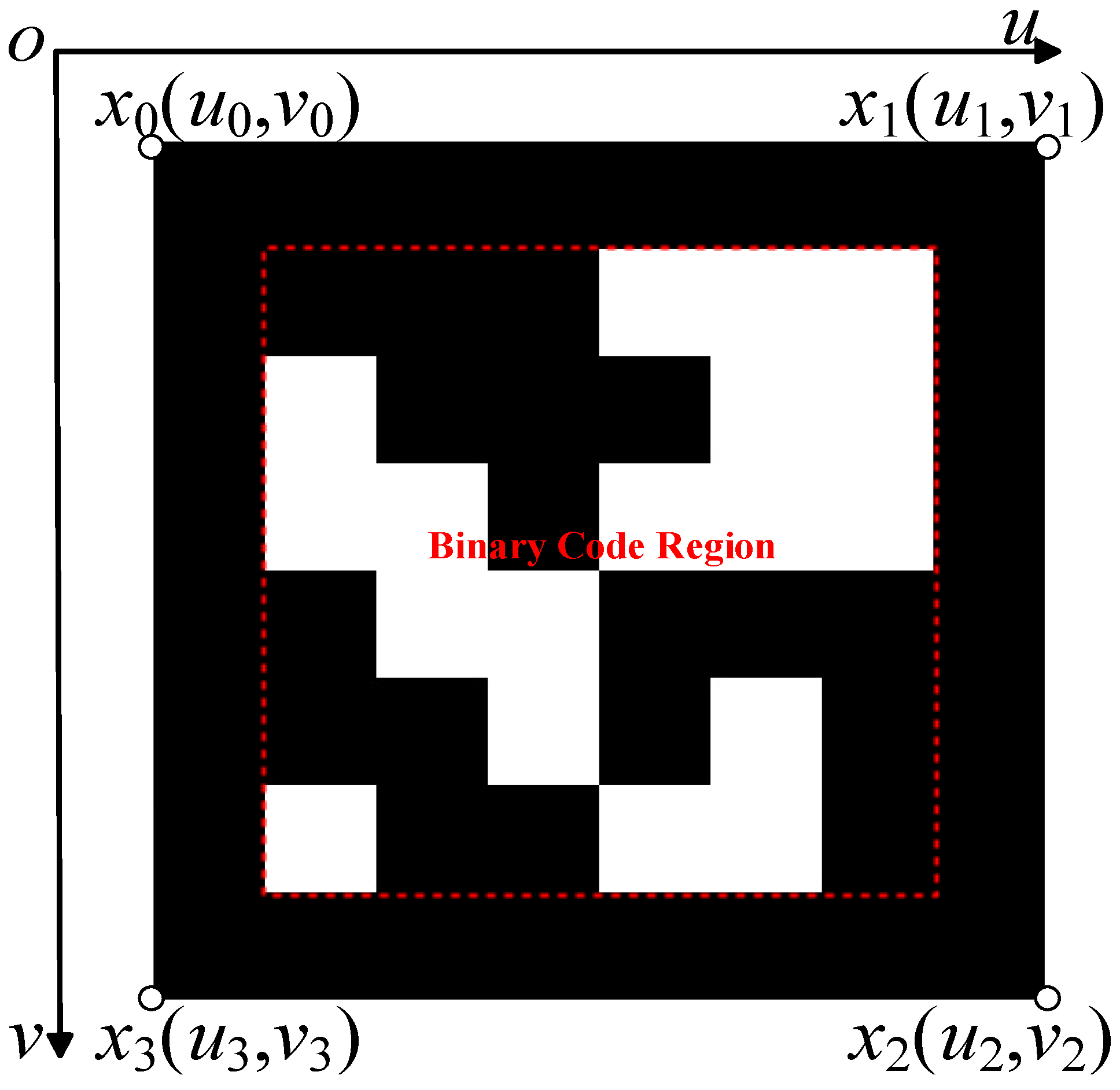
By correcting the tilt [33], the subsequent displacement measurements conducted on the calibrated image can mitigate the adverse effects of the camera’s optical axis not being perpendicular to the measuring surface. This approach enhances the reliability and accuracy of displacement measurements by ensuring that the camera orientation does not introduce significant errors, thereby improving the overall robustness of the deformation monitoring system. Figure 7 illustrates a 6 × 6 ArUco marker, which comprises an outer black border and an internal binary encoding region [34]. Ideally, the ArUco marker is a perfect square; however, in practical scenarios, when the camera’s optical axis is not perpendicular to the measurement plane, the marker is typically projected onto the image plane as a general quadrilateral. Consequently, the ArUco markers in the captured images can be rectified to maintain their square shape, thereby facilitating the correction of image tilt across the entire image. However, our focus is exclusively on the target corner points identified in Section 3.2.2. Therefore, it is sufficient to correct only the pixel coordinates of these specific feature points. This targeted calibration meets the requirements for subsequent deformation measurements while reducing computational overhead, thereby enhancing the efficiency of the deformation monitoring system.

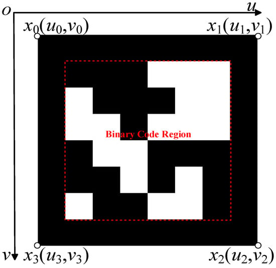
Figure 7. An ArUco marker configured with a 6 × 6 grid and assigned the identifier ID = 0.

In Figure 7, x (u, v) represents the coordinates of the four corner points of the ArUco marker in the pixel coordinate system under general imaging conditions. The Euclidean norms of these coordinates are computed, $‖\left(u_0,v_0\right)-\left(u_1,v_1\right)‖$, $‖\left(u_1,v_1\right)-\left(u_2,v_2\right)‖$, $‖\left(u_2,v_2\right)-\left(u_3,v_3\right)‖$, $‖\left(u_3,v_3\right)-\left(u_0,v_0\right)‖$, and the maximum value among them is designated as X_m. Given that the actual physical edge length of the ArUco marker is L_A, the scaling factor s is calculated using Equation (10):

$$s={\displaystyle \frac{L_A}{X_m}}$$

(10)

The top-left corner of the ArUco marker remains fixed at coordinates x₀ (u₀, v₀). The ideal positions of its four corners are obtained and defined as x_0′ (u₀, v₀), x_1′ (u₀ + Xm, v₀), x_2′ (u₀ + X_m, v₀ + Xm), x_3′ (u₀, v₀ + Xm). Using these correspondences, the projection transformation matrix M can be computed as follows:

$$w’\left(\begin{array}{l}u’\\ v’\\ 1\end{array}\right)=\mathit{{\rm M}}\left(\begin{array}{l}u\\ v\\ 1\end{array}\right)=\left(\begin{array}{ccc}{m}_{11}& m_{12}& m_{13}\\ m_{21}& m_{22}& m_{23}\\ m_{31}& m_{32}& m_{33}\end{array}\right)\left(\begin{array}{l}u\\ v\\ 1\end{array}\right)$$

(11)

In Equation (11), (w’u’, w’v’, w’) represents the homogeneous coordinates after the projection transformation (corresponding to the coordinates of the four corner points of the ArUco under ideal imaging), while (u, v, 1) denotes the homogeneous coordinates before the projection transformation (corresponding to the coordinates of the four corner points in the general imaging case). The elements m_ij are the unknown coefficients to be determined. Leveraging the properties of homogeneous coordinates and setting m₃₃ = 1, the following two linear equations are derived:

$$\left\{\begin{array}{l}u’={\displaystyle \frac{u{m}_{11}+v{m}_{12}+m_{13}}{u{m}_{31}+v{m}_{32}+1}}\\ v’={\displaystyle \frac{u{m}_{21}+v{m}_{22}+m_{23}}{u{m}_{31}+v{m}_{32}+1}}\end{array}\right.$$

(12)

Using the coordinates of the four pairs of corner points of ArUco before and after correction, i.e., (x₀, x_0′), (x₁, x_1′), (x₂, x_2′), (x₃, x_3′), M can be solved. Tilt correction of the target corner point in the markers of an image is applied using M. This calibration process mitigates the stringent requirements for the camera’s installation orientation, thereby enhancing the robustness and accuracy of the deformation monitoring system. Let the calibrated coordinates of two marker points, after applying Equation (12), be denoted as (u_l, v_l) and (u_r, v_r). The actual physical distance between these two marker points can be calculated using Equation (13):

$$D=s‖\left(u_l,v_l\right)-\left(u_r,v_r\right)‖$$

(13)

D denotes the actual straight-line distance between the two measurement points, and s is the scale factor calculated from Equation (10).

3.4. Analysis of Static Detection Experiments

To investigate the impact of subpixel refinement of corner point coordinates on measurement error, as outlined in Section 3.2.3, and to validate the effectiveness of the image tilt correction theory in monocular measurement presented in Section 3.3, we designed the following experiment. Two artificial markers were affixed to a single plane with an actual distance of 140 mm between them. Additionally, an ArUco marker (ID = 0) was placed on the same plane to facilitate subsequent image calibration. The measurement plane was kept fixed while the camera captured images of the plane from different locations, ensuring that its optical axis was not perpendicular to the measurement plane. A total of ten sets of images were acquired. From these, one sample set was selected to demonstrate the comparison of results before and after calibration, as illustrated in Figure 8.

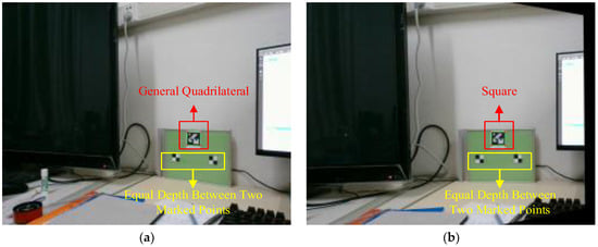
Figure 8. Comparison of calibration results. (a) Pre-calibration. (b) Post-calibration.

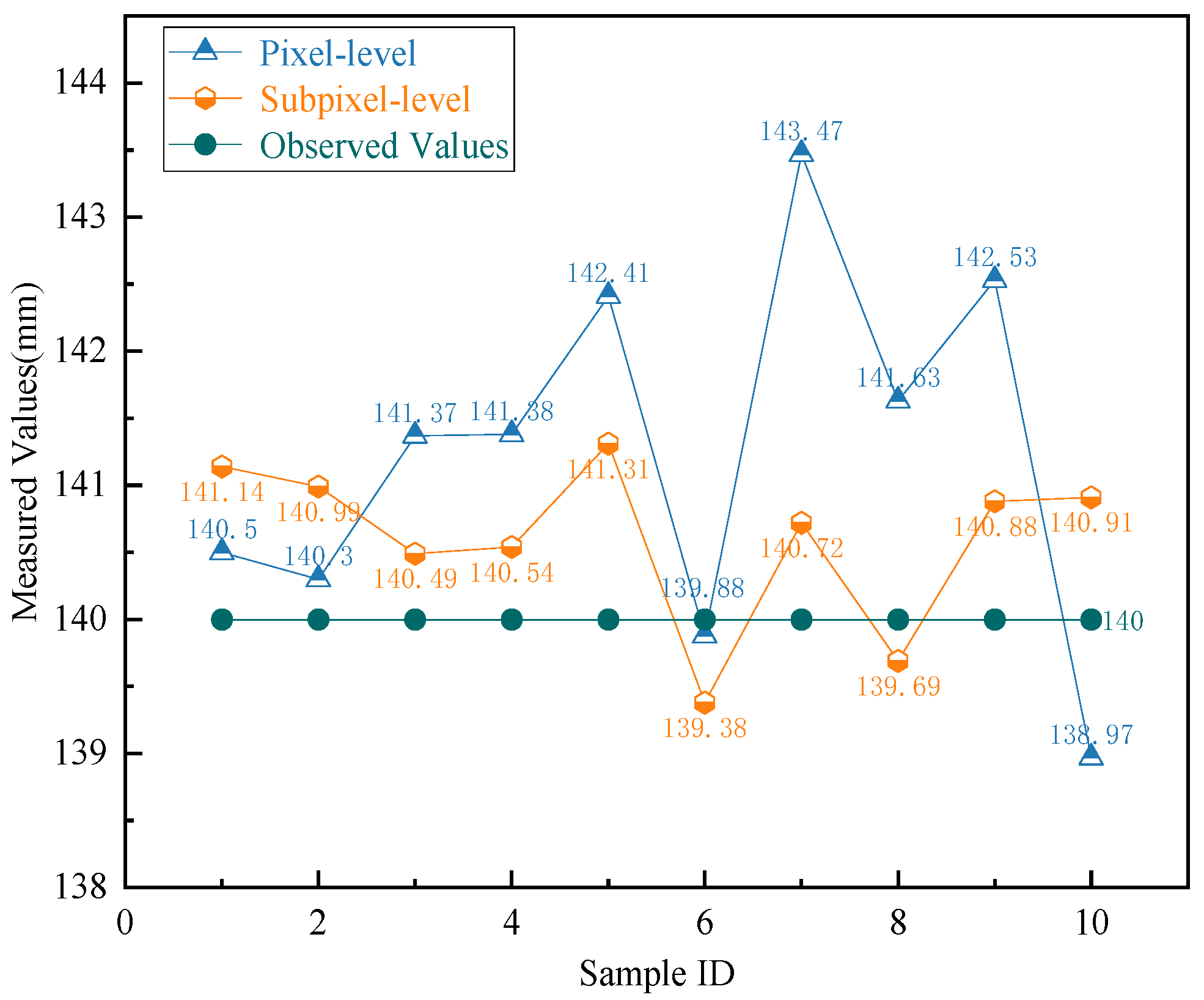
In the experiment, the four corner points of the ArUco markers and the corresponding target corner points were acquired. The application of sub-pixel relocation to these corner points was set as an experimental variable. The actual distance between the target corner points in the two manual markers, as shown in Figure 8, was calculated according to Equation (13). By calculating the distances between the pixel coordinates of the marker points, we obtained the measurement results presented in Figure 9. The results indicate that the image tilt correction technique allows for accurate outcomes even when the camera’s optical axis is not perpendicular to the measurement surface.

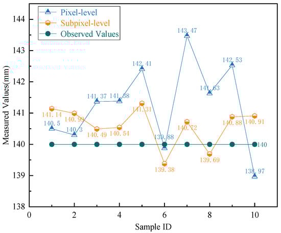
Figure 9. Comparative analysis of measurement results.

While the pixel-level measurements achieved optimal accuracy in Sample Group 6, significant deviations from the actual values were observed in Sample Group 7. In contrast, the subpixel-level measurements exhibited a much smaller range of data fluctuation, indicating higher consistency and precision. To comprehensively evaluate the performance of the measurement methods, the absolute error (AE), mean absolute error (MAE), and the standard deviation of absolute errors (STD) were calculated for the measurement results. These statistical metrics are summarized in Table 1, providing a detailed comparison of the accuracy and robustness of the pixel-level and subpixel-level methods. The sample size of a set of experiments is denoted as n, and x_i (i = 1, 2, … n) represents the measurements obtained through visual methods. The constant μ represents the true value. The Absolute Error (AE) E_i for each measurement, the Mean Absolute Error (MAE) for the dataset, and the Standard Deviation (STD) are calculated using the following formulas:

$$\begin{array}{l}{E}_i=\left|x_i-\mu \right|\\ MAE={\displaystyle \frac{1}{n}}{\displaystyle \sum _{i=1}^n\left|x_i-\mu \right|}\\ STD=\sqrt{{\displaystyle \frac{1}{n}}{\displaystyle \sum _{i=1}^n{(E_i-MAE)}^2}}\end{array}$$

(14)

Table 1. Error statistics for various methods at pixel and subpixel levels.

Method	AE	MAE	STD
Pixel-Level Error	[0.50, 0.30, 1.37, 1.38, 2.41, 0.12, 3.47, 1.63, 2.53, 1.03]	1.474	1.0178
Subpixel-Level Error	[1.14, 0.99, 0.49, 0.54, 1.31, 0.62, 0.72, 0.31, 0.88, 0.91]	0.791	0.2953

As shown in Table 1, while the pixel-level measurement method requires less computational effort, it exhibits larger errors and greater fluctuations. In contrast, the subpixel-level measurement method demonstrates significantly higher accuracy and better data stability, making it more advantageous for practical measurement scenarios. The experimental results validate the accuracy and effectiveness of the proposed method in determining marker point coordinates and actual displacements. These findings highlight the superiority of the subpixel-level approach, particularly in applications requiring precise and reliable deformation measurements.

4. Experimental Analysis of GIL Deformation Measurements

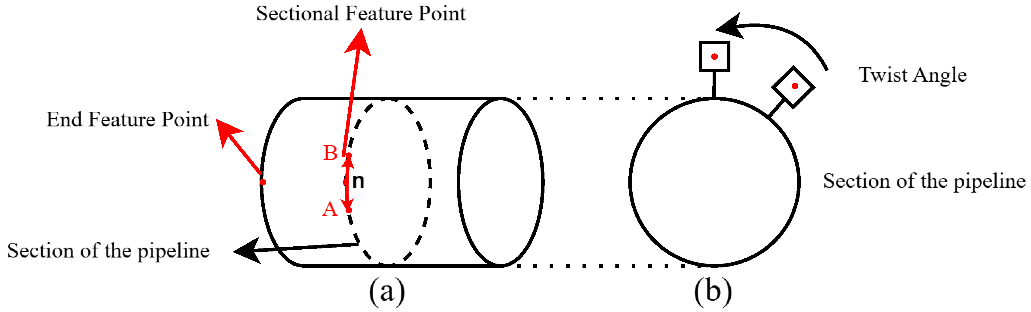
As illustrated in Figure 10a, the measurement point arrangement for evaluating axial strain in pipelines involves selecting a smaller arc segment, AB, on the cross-section. In practical deformation measurements, such an approach can be adopted. Within this segment, n cross-sectional characteristic points and one end characteristic point are positioned, with the end characteristic point assumed to experience no strain. When the pipeline undergoes overall axial rigid body displacement, the rigid displacement is eliminated using the end characteristic point, resulting in the axial displacements at the n characteristic points attributable to pipeline deformation. Building on the findings of reference [22], Equation (15) is employed to define the extent of arc segment AB, thereby assuming that within this segment, the cross-sectional characteristic points lie within the same plane.

$$L_m\le R\sin {10}^{°}$$

(15)

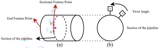
Figure 10. Schematic diagram of measurement point arrangement for pipeline deformation assessment. (a) Axial deformation measurement (b) Torsional deformation measurement.

In Equation (15), R represents the radius of the circle corresponding to arc segment AB, and L_m denotes the perpendicular distance from the midpoint of arc AB to chord AB. As illustrated in Figure 10b, the plane in which the measurement point induces the rotational angle coincides with the pipeline’s cross-sectional plane. When assessing the circumferential torsional deformation of a pipeline, it is assumed that no axial displacement occurs during the measurement period.

4.1. Axial Deformation Measurement at a Single Feature Point

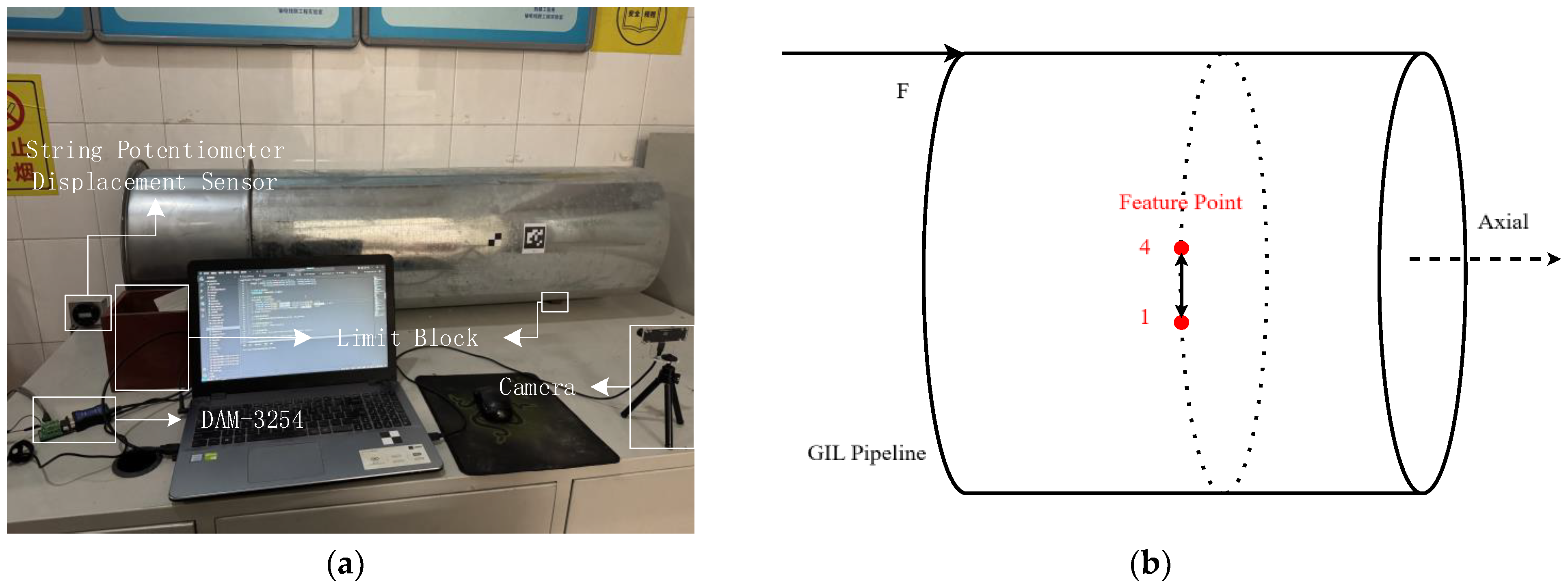
To evaluate the proposed methodology, a simulation experiment was conducted using a pipeline structure similar to the GIL pipeline. In the simulation experiment, the displacement of a measurement point was measured and verified. To facilitate the validation of visual measurement results, limiting blocks were employed to constrain the pipeline’s displacement along the axial direction. During the experiment, axial force was applied to the simulated pipeline, inducing axial displacement. The deformation monitoring process was simulated by tracking the displacement changes at the target corner point. The experimental simulation setup is shown in Figure 11. To verify the accuracy of the proposed method, data acquisition was performed using both a displacement sensor and a camera. The displacement sensor operated at a sampling frequency of 600 Hz. To ensure synchronization, the camera is fixed in position throughout each measurement session. Initially, while the pipeline is stationary, a reference image is captured. Next, the pipeline is subjected to a controlled axial displacement, and the system is allowed to reach a new stationary state. Once the sensor’s displacement reading stabilizes, a subsequent image is taken. The displacement relative to the initial state is then determined by comparing the two images. Under these stationary conditions, the visual measurement aligns with the sensor’s reading. This ensures an accurate correspondence between the displacement measured by the vision system and that recorded by the sensor. Using this method, a total of 10 sets of images were obtained, with the initial image corresponding to a displacement of 0. Consequently, nine sets of displacement comparisons were acquired. This synchronization was critical for aligning the data streams and enabling a precise comparison of the measurement results. This experimental setup allowed for a controlled assessment of the proposed method’s precision and reliability under conditions mimicking real-world pipeline deformation scenarios.

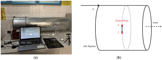
Figure 11. Simulation experimental platform. (a) Schematic diagram of the operation. (b) Equipment arrangement.

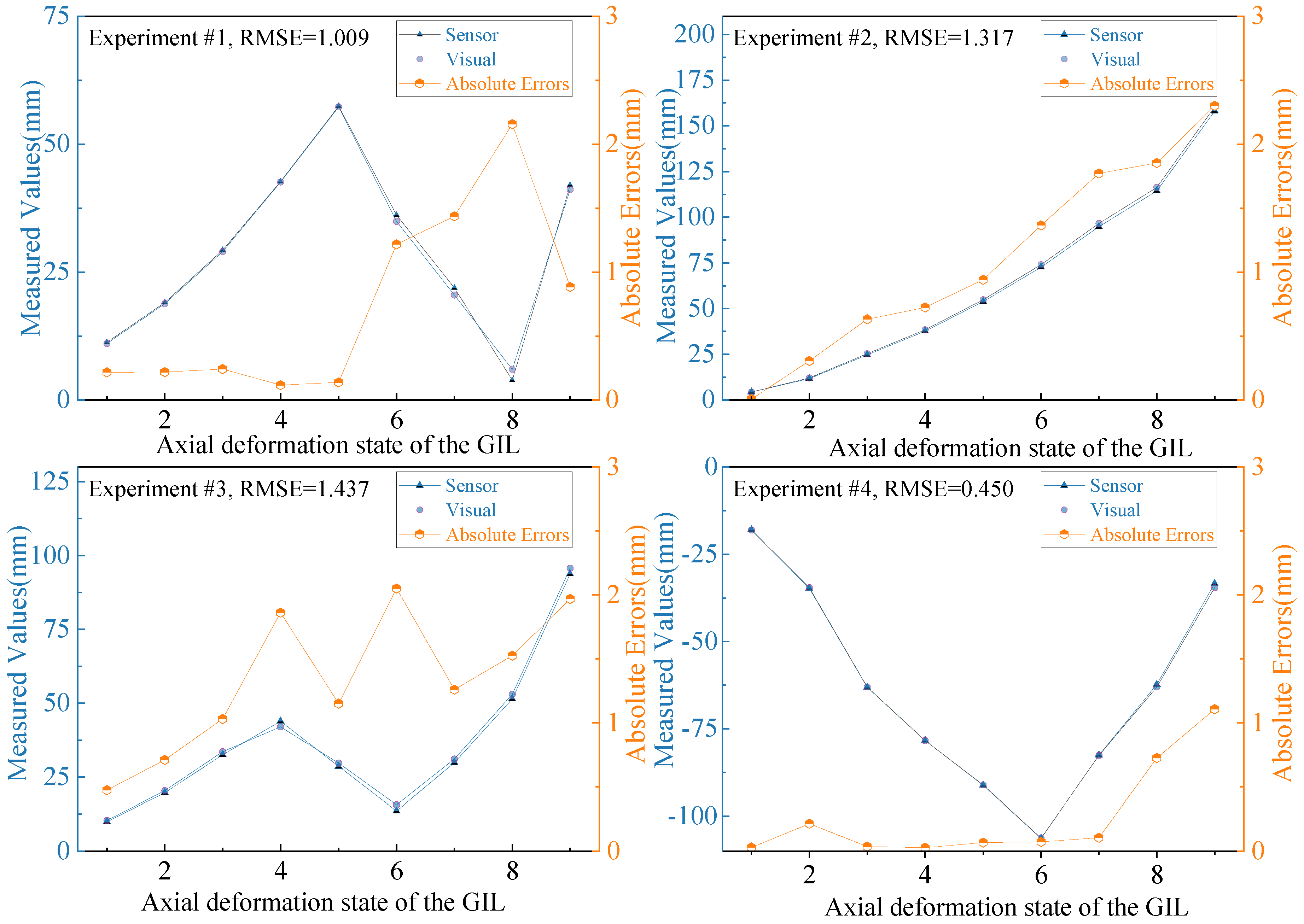
The experiment was conducted four times to validate the robustness of the proposed measurement method. For each trial, varying magnitudes and directions of force were applied to the pipeline. Additionally, the pipeline was rotated appropriately to alter its orientation, thereby creating different angles between the camera and the measurement marker plane, as well as varying the distance between the camera and the target. These variations introduced diverse measurement conditions, enabling a comprehensive assessment of the method’s adaptability. The measurement results, shown in Figure 12, illustrate the displacement from the initial position. The data reflects the performance of the proposed method under varying experimental conditions, demonstrating its ability to adapt to changes in camera orientation and distance while maintaining measurement accuracy.

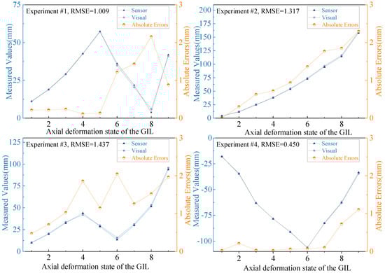
Figure 12. Results of simulation measurements.

To verify the accuracy of the visual measurement method, the measurements obtained from the wire-type displacement sensor were used as the reference. For a more intuitive presentation of the results, key metrics from the four experimental trials are summarized in Table 2. These metrics include the maximum absolute error (MaxAE), the mean absolute error (MAE1), the computation time per frame, and the root mean square error (RMSE). In a measurement, the amount of collected data is n. Let y_i (i = 1, 2, …, n) represent the measured values obtained by the visual method, and y_i′ represent the true values corresponding to the measured values. Then the MaxAE, MAE1, and RMSE of this set of data are determined by the following equations:

$$\begin{array}{l}\mathrm{MaxAE}=\max (\left|y_i-y_i’\right|,i=1,2,\dots n)\\ \mathrm{MAE}1={\displaystyle \frac{1}{n}}{\displaystyle \sum _{i=1}^n\left|y_i-y_i’\right|}\\ RMSE=\sqrt{{\displaystyle \frac{1}{n}}{\displaystyle \sum _{i=1}^n{\left(y_i-y_i’\right)}^2}}\end{array}$$

(16)

Table 2. Statistical analysis of visual measurement errors and time consumption.

Experimental Group	MaxAE (mm)	MAE1 (mm)	RMSE (mm)	Time Consumption (s/Frame)
1	2.156	0.736	1.009	0.024
2	2.301	1.099	1.317
3	2.052	1.337	1.437
4	1.107	0.265	0.450

The experimental results indicate that variations in applied forces, angles, and distances did not significantly impact measurement accuracy. The observed measurement errors remained consistently low, demonstrating the stability and reliability of the proposed method. The method proposed in reference [12] utilizes a multi-camera setup for 3D coordinate measurements, which monitors the displacement of markers affixed to the pipeline to assess GIL deformation, achieving a mean absolute error of less than 3 mm. In contrast, the monocular vision measurement method proposed in this study is simpler and more convenient. As shown in Table 2, the proposed method achieved a mean absolute error of no more than 1.337 mm across multiple measurements, with the minimum average absolute error being 0.265 mm. These results highlight the high accuracy of the proposed method. By flexibly positioning artificial markers, the method can adapt to various deformation scenarios in GIL pipelines. Moreover, improving the precision of the artificial markers and enhancing camera performance could further increase the accuracy of the measurements. Additionally, the average computation time per frame is approximately 0.024 s, demonstrating that the method is capable of real-time continuous measurement. The calculated corner coordinates of the artificial markers are unique, indicating that the measurement system achieves automated measurements, reduces human intervention, and offers significant practical value for real-world applications.

4.2. Torsional Deformation Measurements

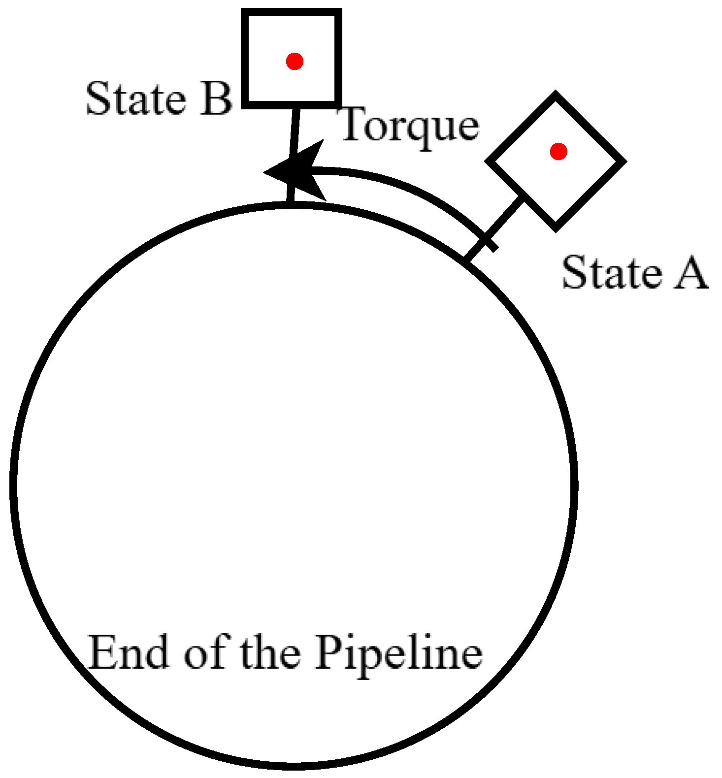
To simulate the torsional deformation of actual pipelines, we measure the rotational angle of a rigid body about its axis. Specifically, we focus on measuring the rotation angle at a particular point on the cross-section. By manually applying torque at one end and utilizing the limit blocks illustrated in Figure 11, we ensure that the pipeline undergoes pure rigid-body rotation. An operational schematic is presented in Figure 13.

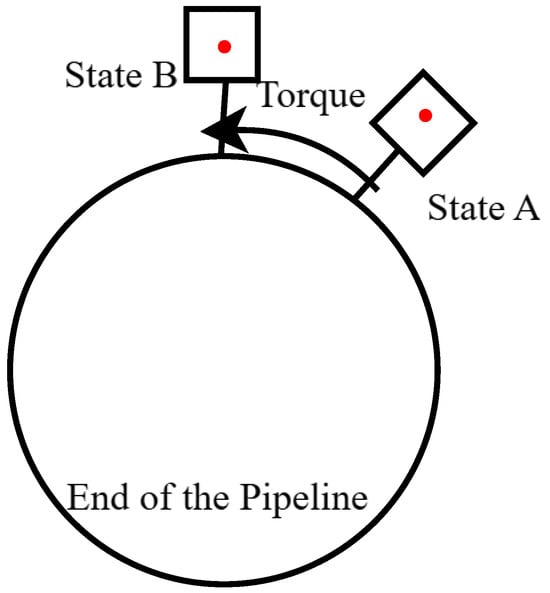
Figure 13. Operational schematic.

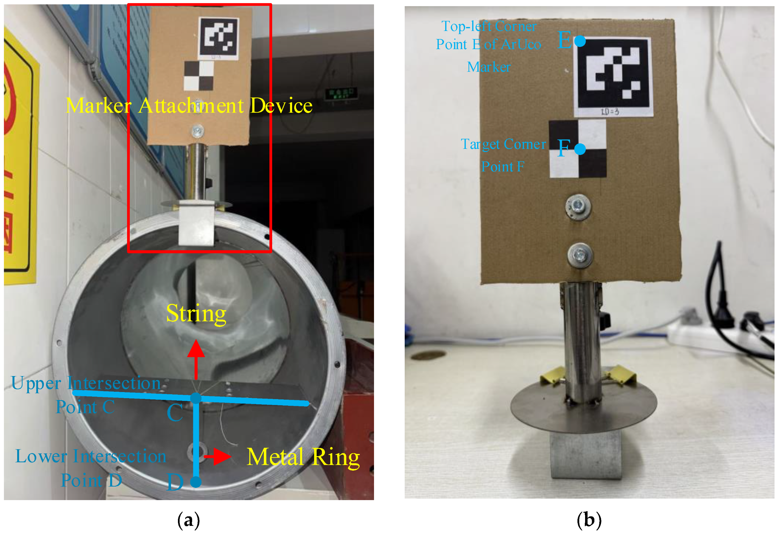
Additional experimental equipment includes a marker fixation device, protractor, string, and metal rings, with the experimental setup arranged as illustrated in Figure 14. The T-shaped welding platform shown in Figure 14a positions the line segment CD along the diameter of the end face circle. One end of the string is connected to the metal ring, while the other end is secured at point C. Under the influence of gravity, the string remains taut and vertically aligned, facilitating the measurement of the actual rotation angle. In the marker fixation device depicted in Figure 14b, point E corresponds to the upper-left corner of the ArUco marker, and point F represents the target corner point of the extracted marker. The mechanical structure ensures that both line segments EF and CD lie along the diameter of the end face circle.

Figure 14. Experimental apparatus layout. (a) End of the pipeline. (b) Marker fixation device.

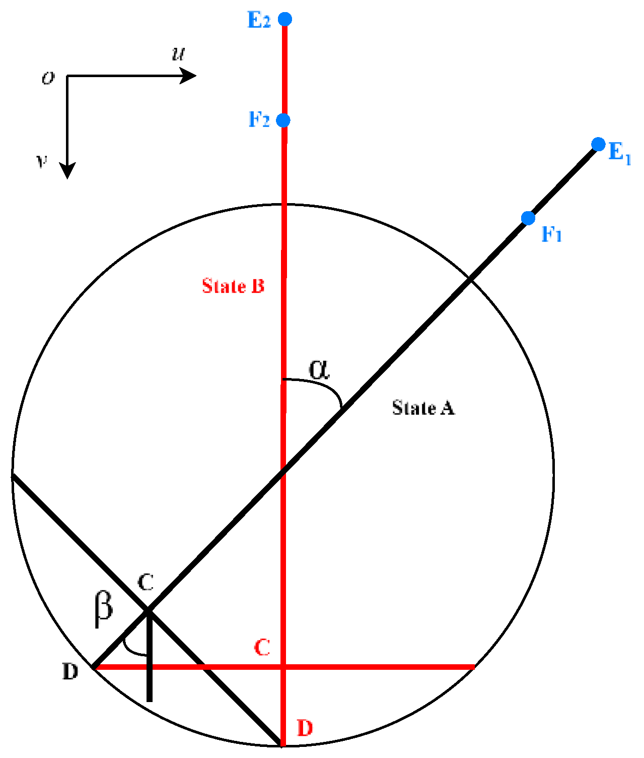
To facilitate the validation of the visual measurement accuracy for rotational angles, a static measurement approach was employed. As illustrated in Figure 13, the rotational angle was measured from a completely stationary state A to a completely stationary state B. The geometric relationships involved in calculating the rotational angle during visual measurements are depicted in Figure 15.

Figure 15. Geometric relationships in rotation angle calculation.

Due to the geometric configuration, the angles α and β are equal. Therefore, measuring the β value at point C suffices to verify the accuracy of the visually measured rotation angle. Within the image pixel coordinate system under ouv, the rotation angle α is computed using Equation (17).

$$\alpha =\arccos \left({\displaystyle \frac{\overrightarrow{F_1{E}_1}•\overrightarrow{F_2{E}_2}}{\left|\overrightarrow{F_1{E}_1}\right|\left|\overrightarrow{F_2{E}_2}\right|}}\right)$$

(17)

The vectors F₁E₁ and F₂E₂ are calculated through points F and E in the pixel coordinates of the ouv coordinate system.

The camera was strategically positioned approximately 1.7 m from the measurement plane. Images of the pipe end face were captured under seven distinct states, with each state corresponding to a specific rotational angle increment. The coordinates of points E and F for each state are recorded in Table 3, with all values presented to two decimal places.

Table 3. Pixel coordinates of points E and F.

State	The Pixel Coordinates of Point F Before Calibration	The Pixel Coordinates of Point F After Calibration	The Pixel Coordinates of Point E Before Calibration	The Pixel Coordinates of Point E After Calibration
0	(1018.95, 432.81)	(1026.08, 434.75)	(1027.00, 356.45)	(1027.00, 356.45)
1	(1031.53, 434.34)	(1039.05, 435.22)	(1042.90, 357.44)	(1042.80, 355.72)
2	(1042.99, 436.02)	(1050.98, 435.95)	(1055.70, 359.64)	(1055.80, 356.51)
3	(1056.41, 437.43)	(1064.99, 436.23)	(1073.10, 362.40)	(1073.40, 357.39)
4	(1072.35, 439.97)	(1081.89, 437.48)	(1092.90, 365.29)	(1093.90, 358.13)
5	(1103.15, 447.73)	(1115.45, 443.02)	(1130.10, 374.94)	(1133.50, 363.85)
6	(1130.24, 457.63)	(1146.08, 451.37)	(1162.40, 386.82)	(1169.40, 372.57)

In Table 3, the pixel coordinates of point E remain unchanged before and after calibration. The coordinates of points E and F in states 1–6 are corrected using the correction matrix M of the 0-state image. The coordinates of point E in state 0 are unchanged before and after correction. This stability is attributed to the image tilt correction theory discussed in Section 3.3, where point E serves as the reference point for the projection transformation. Utilizing Equation (17), the angles between each pair of states were calculated (α). The angles before image calibration (pre-α) and their absolute errors (pre-AE) were computed, as well as the angles after image calibration (post-α) and their absolute errors (post-AE). The calculated results, along with the actual measurements, are summarized in Table 4, with all values rounded to two decimal places. Table 4 presents the angle value.

Table 4. Angle Values.

State	Measured Values (°)	Pre-α (°)	Pre-AE (°)	Post-α (°)	Post-AE (°)
1	2.0	2.39	0.39	2.03	0.03
2	1.5	1.03	0.47	0.77	0.73
3	2.7	3.10	0.40	2.62	0.08
4	2.8	2.84	0.04	2.52	0.28
5	4.5	4.93	0.43	4.24	0.26
6	4.1	4.11	0.01	3.64	0.46
MAE	-	-	0.29	-	0.31

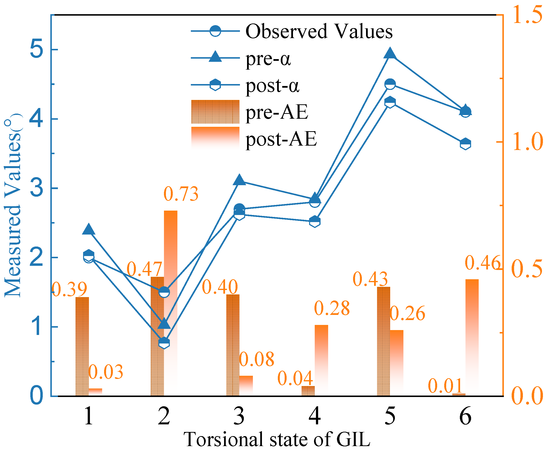
To clearly illustrate the variations in the measurement results, the data from Table 4 are depicted in Figure 16. As shown in Figure 16, using the experimentally measured range of rotation angles as an example, directly converting the actual rotation angle from the pixel coordinates provides relatively accurate results, with the maximum deviation from the actual value being less than 0.5°. This finding also suggests that the camera’s optical axis is nearly perpendicular to the measurement plane. After applying the correction, the measured rotation angles deviate only slightly from the actual values. The largest error, 0.73°, occurs between State 1 and State 2, indicating that this tilt correction technique is also effective for measuring torsional deformation angles in GIL. In reference [35], the authors employed binocular digital image correlation technology to measure the shear angle of torsional deformation in carbon steel cylinders, achieving an MAE of 0.35°, which adequately meets measurement needs. Based on the measurement data from the reference, this study introduces a new measurement method for the torsional deformation of GIL, achieving an MAE of 0.31° within a certain measurement range. This method is considered to be an effective measurement approach to some extent, although the specific applicable measurement range requires further investigation.

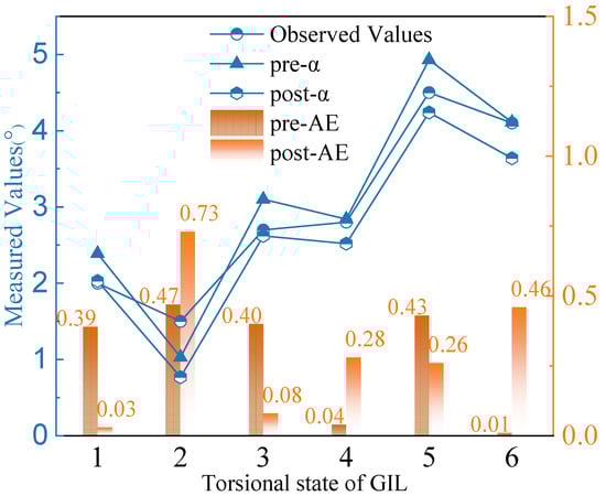
Figure 16. Comparison of measured angles.

5. Conclusions

Based on the characteristics of GIL pipelines, this study integrates the constructed YOLOv10 model, high-precision corner detection methods, and image tilt correction techniques to propose an automated, real-time monitoring method for GIL pipeline deformation. The key conclusions of the research are as follows:

(1)

To address the limitations of traditional FAST corner detection methods, an adaptive threshold calculation method was developed. Combined with the Shi–Tomasi algorithm, redundant corner points were effectively removed, enabling the automated extraction and tracking of the target corner point at the center of the marker. Experiments verified the effectiveness of the proposed image tilt correction theory in monocular measurement and analyzed the impact of subpixel refinement on measurement error. The results show that, after image correction, measurement accuracy became insensitive to the camera’s orientation. The pixel-level measurement method achieved a mean absolute error (MAE) of 1.474 mm with a standard deviation of 1.0178 mm, while the subpixel-level measurement method improved the MAE to 0.791 mm with a standard deviation of 0.2953 mm. This demonstrates that the subpixel-level method offers higher measurement precision and better data stability, making it advantageous for practical measurement scenarios.

(2)

Simulated deformation experiments verified the robustness, precision, real-time capability, and automation of the proposed monitoring system. The results indicate that the system is insensitive to changes in pipeline loading conditions and camera orientation. The average absolute error of the measurements did not exceed 1.337 mm, with the minimum average absolute error being 0.265 mm, meeting the required measurement accuracy. Furthermore, the computation time per frame was approximately 0.024 s, enabling real-time, automated deformation monitoring.

(3)

The proposed GIL pipeline deformation measurement method was validated through torsional deformation experiments. When the camera was positioned approximately 1.7 m from the measurement plane, the maximum average absolute error did not exceed 0.31°. It is important to note that, regardless of whether axial or torsional deformation is being measured, the projective transformation matrix M should always be calculated from the first image acquired during each measurement session. This same matrix should then be applied to all subsequent images, ensuring consistent and accurate correction.

In this study, we selected a camera with less distortion. Although the current work does not delve deeply into intrinsic camera calibration, future research will explore comprehensive calibration methods to further enhance measurement accuracy without increasing manual intervention. Additionally, further optimization of the YOLO-based model will also be pursued to enhance its specificity for GIL deformation, improve the speed of region of interest extraction, and reduce computational overhead. Exploring multi-camera systems and alternative AI techniques will also be considered to more effectively capture three-dimensional deformations.

References

- Xiao, S.; Zhang, X.; Tang, J.; Liu, S. A review on SF6 substitute gases and research status of CF3I gases. Energy Rep. 2018, 4, 486–496. [Google Scholar] [CrossRef]
- Magier, T.; Tenzer, M.; Koch, H. Direct Current Gas-Insulated Transmission Lines. IEEE Trans. Power Deliv. 2018, 33, 440–446. [Google Scholar] [CrossRef]
- Tu, Y.; Chen, G.; Li, C.; Wang, C.; Ma, G.; Zhou, H.; Ai, X.; Cheng, Y. ±100-kV HVDC SF6/N2 Gas-Insulated Transmission Line. IEEE Trans. Power Deliv. 2020, 35, 735–744. [Google Scholar] [CrossRef]
- Shu, Q.; Huang, Z.; Yuan, G.; Ma, W.; Ye, S.; Zhou, J. Impact of wind loads on the resistance capacity of the transmission tower subjected to ground surface deformations. Thin-Walled Struct. 2018, 131, 619–630. [Google Scholar] [CrossRef]
- Fu, X.; Du, W.-L.; Li, H.-N.; Li, G.; Dong, Z.-Q.; Yang, L.-D. Stress state and failure path of a tension tower in a transmission line under multiple loading conditions. Thin-Walled Struct. 2020, 157, 107012. [Google Scholar] [CrossRef]
- Tan, X.; Poorghasem, S.; Huang, Y.; Feng, X.; Bao, Y. Monitoring of pipelines subjected to interactive bending and dent using distributed fiber optic sensors. Autom. Constr. 2024, 160, 105306. [Google Scholar] [CrossRef]
- Yang, L.; Fan, J.; Liu, Y.; Li, E.; Peng, J.; Liang, Z. A Review on State-of-the-Art Power Line Inspection Techniques. IEEE Trans. Instrum. Meas. 2020, 69, 9350–9365. [Google Scholar] [CrossRef]
- Yang, Y.; Wang, M.; Wang, X.; Li, C.; Shang, Z.; Zhao, L. A Novel Monocular Vision Technique for the Detection of Electric Transmission Tower Tilting Trend. Appl. Sci. 2023, 13, 407. [Google Scholar]
- Wang, D.; Yue, J.; Li, J.; Xu, Z.; Zhao, W.; Zhu, R. Research on sag monitoring of ice-accreted transmission line arcs based on stereovision technique. Electr. Power Syst. Res. 2023, 225, 109794. [Google Scholar] [CrossRef]
- Zhang, K.; Liu, J.; Li, Y.; Sun, C.; Zhang, L. Research on Improving Denoising Performance of ROI Computer Vision Method for Transmission Tower Displacement Identification. Energies 2023, 16, 539. [Google Scholar] [CrossRef]
- Li, J.; Zheng, H.; Liu, P.; Liang, Y.; Shuang, F.; Huang, J. Safety monitoring method for powerline corridors based on single-stage detector and visual matching. High. Volt. 2024, 9, 805–815. [Google Scholar] [CrossRef]
- Fauzan, K.N.; Suwardhi, D.; Murtiyoso, A.; Gumilar, I.; Sidiq, T.P. Close-range photogrammetry method for SF6 Gas Insulated Line (GIL) deformation monitoring. Int. Arch. Photogramm. Remote Sens. Spatial Inf. Sci. 2021, XLIII-B2-2021, 503–510. [Google Scholar] [CrossRef]
- Xu, Y.; Brownjohn, J.; Kong, D. A non-contact vision-based system for multipoint displacement monitoring in a cable-stayed footbridge. Struct. Control Health Monit. 2018, 25, e2155. [Google Scholar] [CrossRef]
- Brownjohn, J.M.W.; Xu, Y.; Hestr, D. Vision-based bridge deformation monitoring. Front. Built Environ. 2017, 3, 23. [Google Scholar] [CrossRef]
- Yang, Y.; Ma, T.; Du, S. Robust template matching with angle location using dynamic feature pairs updating. Appl. Soft Comput. 2019, 85, 105804. [Google Scholar] [CrossRef]
- Wu, T.; Dong, Y. YOLO-SE: Improved YOLOv8 for remote sensing object detection and recognition. Appl. Sci. 2023, 13, 12977. [Google Scholar] [CrossRef]
- Li, Y.; Liu, W.; Li, L.; Zhang, W.; Xu, J.; Jiao, H. Vision-based target detection and positioning approach for underwater robots. IEEE Photonics J. 2022, 15, 8000112. [Google Scholar] [CrossRef]
- Yang, H.; Chen, L.; Chen, M.; Ma, Z.; Deng, F.; Li, M.; Li, X. Tender tea shoots recognition and positioning for picking robot using improved YOLO-V3 model. IEEE Access 2019, 7, 180998–181011. [Google Scholar] [CrossRef]
- Bansal, M.; Kumar, M.; Kumar, M. 2D object recognition: A comparative analysis of SIFT, SURF and ORB feature descriptors. Multimed. Tools Appl. 2021, 80, 18839–18857. [Google Scholar] [CrossRef]
- Li, Y.; Zheng, W.; Liu, X.; Mou, Y.; Yin, L.; Yang, B. Research and improvement of feature detection algorithm based on FAST. Rend. Lincei 2021, 32, 775–789. [Google Scholar] [CrossRef]
- Zhuang, Y.; Chen, W.; Jin, T.; Chen, B.; Zhang, H.; Zhang, W. A Review of Computer Vision-Based Structural Deformation Monitoring in Field Environments. Sensors 2022, 22, 3789. [Google Scholar] [CrossRef] [PubMed]
- Choi, I.; Kim, J.; Kim, D. A target-less vision-based displacement sensor based on image convex hull optimization for measuring the dynamic response of building structures. Sensors 2016, 16, 2085. [Google Scholar] [CrossRef] [PubMed]
- Shan, W.; Bai, F.; Xu, Y.; Gao, X.; Li, P. Perspective deformation correction for circular pointer meter based on prior indication structure feature. Measurement 2024, 229, 114423. [Google Scholar] [CrossRef]
- Barath, D. On Making SIFT Features Affine Covariant. Int. J. Comput. Vis. 2023, 131, 2316–2332. [Google Scholar] [CrossRef]
- Yang, Z.; Shen, D.; Yap, P.-T. Image mosaicking using SURF features of line segments. PLoS ONE 2017, 12, e0173627. [Google Scholar] [CrossRef]
- Damaneh, M.M.; Mohanna, F.; Jafari, P. Static hand gesture recognition in sign language based on convolutional neural network with feature extraction method using ORB descriptor and Gabor filter. Expert. Syst. Appl. 2023, 211, 118559. [Google Scholar] [CrossRef]
- Wang, A.; Chen, H.; Liu, L.; Chen, K.; Lin, Z.; Han, J.; Ding, G. YOLOv10: Real-Time End-to-End Object Detection. arXiv 2024, arXiv:2405.14458. [Google Scholar]
- Lee, Y.H.; Chen, T.C.; Liang, H.C.; Liao, J.X. Algorithm and Architecture Design of FAST-C Image Corner Detection Engine. IEEE Trans. Very Large Scale Integr. (VLSI) Syst. 2021, 29, 788–799. [Google Scholar] [CrossRef]
- Hong, Q.; Jiang, H.; Xiao, P.; Du, S.; Li, T. A Parallel Computing Scheme Utilizing Memristor Crossbars for Fast Corner Detection and Rotation Invariance in the ORB Algorithm. IEEE Trans. Comput. 2024, 74, 996–1010. [Google Scholar] [CrossRef]
- Bansal, M.; Kumar, M.; Kumar, M.; Kumar, K. An efficient technique for object recognition using Shi-Tomasi corner detection algorithm. Soft Comput. 2021, 25, 4423–4432. [Google Scholar] [CrossRef]
- Zhu, Q.; Wu, B.; Wan, N. A sub-pixel location method for interest points by means of the Harris interest strength. Photogramm. Rec. 2007, 22, 321–335. [Google Scholar] [CrossRef]
- Xie, X.; Ge, S.; Xie, M.; Hu, F.; Jiang, N. An improved industrial sub-pixel edge detection algorithm based on coarse and precise location. J. Ambient. Intell. Humaniz. Comput. 2020, 11, 2061–2070. [Google Scholar] [CrossRef]
- Liu, Y.; Su, X.; Guo, X.; Suo, T.; Yu, Q. A novel concentric circular coded target, and its positioning and identifying method for vision measurement under challenging conditions. Sensors 2021, 21, 855. [Google Scholar] [CrossRef]
- Becerra, L.L.; Ferrua, J.A.; Drake, M.J.; Kumar, D.; Anders, A.S.; Wang, E.N.; Preston, D.J. Active fume hood sash height monitoring with audible feedback. Energy Rep. 2018, 4, 645–652. [Google Scholar] [CrossRef]
- Wang, L.; Feng, Y. An Adaptive Window Shape-Based DIC Method for Large Torsional Deformation Measurement. IEEE Trans. Instrum. Meas. 2023, 72, 5004510. [Google Scholar] [CrossRef]
Disclaimer/Publisher’s Note: The statements, opinions and data contained in all publications are solely those of the individual author(s) and contributor(s) and not of MDPI and/or the editor(s). MDPI and/or the editor(s) disclaim responsibility for any injury to people or property resulting from any ideas, methods, instructions or products referred to in the content. |
© 2025 by the authors. Licensee MDPI, Basel, Switzerland. This article is an open access article distributed under the terms and conditions of the Creative Commons Attribution (CC BY) license (https://creativecommons.org/licenses/by/4.0/).