Research on the Quantitative Impact of Power Angle Oscillations on Transient Voltage Stability in AC/DC Receiving-End Power Grids

Abstract

In practical engineering, it has been observed that increasing local generators’ capacity in receiving-end power grids can lead the system to transition from voltage instability to power angle instability after a fault. This contradicts the typical engineering experience, where increasing the generators’ capacity at the receiving end is expected to enhance voltage stability, making it challenging to define an appropriate pre-control range for generators. This paper aims to quantify the impact of local generators on the stability of AC/DC receiving-end power grids. First, the paper describes the instability phenomena observed under different generators’ capacity conditions in actual AC/DC receiving-end power grids. Next, by using a simplified single-machine-load-infinite-bus model, the paper explores how the system’s instability characteristics evolve from being dominated by load instability to being driven by generator instability as the ratio of local generators to load varies. This study conducts an in-depth analysis of the coupling mechanism between power angle stability and voltage stability. For the first time, it quantitatively characterizes the stable operating region of the system using power angle and induction motor slip as dual constraint conditions, providing a new theoretical framework for power system stability analysis. Additionally, addressing the lack of quantitative research on the upper limit of generator operation in current systems, this study constructs post-fault power recovery curves for loads and DC power sources. Based on the equal-area criterion, it proposes a quantitative index for the upper limit of local generator operation, filling a research gap in this field and providing a crucial theoretical basis and reference for practical power system operation and dispatch.

1. Introduction

With the continuous expansion of long-distance HVDC transmission, the hybrid AC/DC characteristics of power grids have become more prominent [1,2]. The voltage stability of the AC/DC receiving-end grid has become an increasingly critical issue due to factors such as load growth and DC power injections [3]. Increasing local generators’ capacity is one of the measures to improve voltage stability at the receiving end of the grid. The more local generators’ capacity is online, the stronger the voltage support capability of the system, and the better the system’s ability to withstand disturbances following a fault. However, in practical engineering, it is found that the power angle and voltage of the system are unstable at the same time after a fault despite the increase in the local generators’ capacity. This creates difficulties in defining an appropriate operational pre-control interval for generators’ capacity, posing a significant threat to the safe and stable operation of the power system.

Many scholars have conducted research from various perspectives to address the voltage stability issues of the receiving-end grid. One of the key factors influencing voltage instability is the dynamic characteristics of the load, with the main dynamic component of the load being the induction motor. Some studies have established a method for determining the operating state of induction motors by constructing the stability boundary on the load bus P-V plane and comparing the operating point with the boundary. This approach provides an intuitive explanation for short-term voltage instability phenomena [4]. In reference [5], a third-order induction motor load model was used to simulate and analyze the impact of different induction motor parameters on voltage stability. References [6,7] studied the analytical method for determining the limit removal time of induction motors, aiming to reflect the transient voltage stability conditions at different load nodes. Reference [8] investigated the transient voltage instability mechanism of induction motors from the perspective of network apparent power transmission. Regarding DC voltage stability, reference [9] conducts an in-depth theoretical investigation into voltage instability caused by the aggregation of multiple induction motor loads. Reference [10] proposes a full-state embedding solution that effectively addresses both steady-state and dynamic issues in systems containing induction motors. Additionally, some studies combine sensitivity analysis with the modal method to assess static voltage and power stability in multi-infeed DC systems [11]. References [12,13,14] used the short-circuit ratio index to characterize the static voltage stability of DC multi-infeed systems. References [15,16] simulated and analyzed the mechanism of transient voltage instability in the receiving-end grid caused by DC power injection, and proposed stability control measures. Reference [17] analyzed the recovery characteristics of DC systems after faults and proposed a two-stage transient voltage evaluation method based on multi-binary table criteria.

Existing research on generator operation ranges in power grids has primarily focused on determining the minimum generators’ capacity requirements. Reference [18] based on the local power supply structure and load characteristics of Shanghai, calculates the minimum startup scale under different peak load levels using voltage stability constraints. Reference [19] analyzes system stability under different power flow scenarios and generators’ capacity conditions in the Hubei power grid by simulating critical operating modes. It identifies the minimum startup boundary following an N-2 contingency at the Jing zhou side of the Jing-Wu double-circuit transmission line. From the perspective of short-circuit indices, reference [20] develops a minimum startup calculation method for areas near HVDC systems in the Zhe jiang power grid by analyzing the interactive effects of nearby ultra-high voltage DC (UHVDC) transmission. This method considers critical commutation failure faults and short-circuit current contributions. Reference [21] proposes an analytical algorithm for sectional power limits that accounts for short-circuit capacity, achieving precise calculations by incorporating security and stability constraints along with generator short-circuit capacity contribution indices. Reference [22] establishes a coupling model between conventional modes and system strength and introduces an optimization model aimed at maximizing renewable energy integration. A hybrid solving strategy combining genetic algorithms and the CPLEX solver is employed to optimize the solution. Beyond short-circuit indices, researchers have proposed various methods for determining the minimum generators’ capacity requirements. Reference [23] introduces a comprehensive quantitative index that incorporates electrical distance and dynamic reactive power response by identifying heavily loaded regions and weak nodes, optimizing the startup sequence of generators. Reference [24] defines key transient voltage recovery period indicators and develops an iterative search-based method for determining the minimum generators’ capacity scheme, enabling rapid identification of the optimal startup configuration for receiving-end power grids. Reference [25] explored the minimum generators’ capacity calculation method under the voltage stability requirements of DC and renewable energy sources. Some studies have further found that excessive generators’ capacity can lead to the coupling instability of the power angle and voltage. Reference [26] highlights that mid-to-long-term voltage instability may cause generators to lose their equilibrium points, potentially leading to transient power angle instability. Reference [27] proposed a method for identifying the dominant instability mode by extracting the dominant variables that reflect the system’s in-stability patterns. Reference [28] suggested an emergency control strategy to reduce the system’s instability risk caused by power angle–voltage coupling instability. Reference [29] analyzed the interaction between power angle instability and induction motor instability, pointing out that after a fault, the swinging of the machine group’s power angle can cause a reduction in the system’s equivalent potential, leading to voltage instability. Reference [30] further proposed a quantitative evaluation index for the coupling intensity between power angle and voltage. References [31,32] established power angle–voltage coupling instability evaluation models from the perspective of artificial intelligence. Regarding the decoupling analysis of dynamic characteristics, while singular perturbation theory can be applied to separate the dynamic processes of mid-to-long-term voltage stability and transient power angle stability, its application in transient voltage and power angle stability analysis remains limited [33]. Current research primarily analyzes the impact of various factors on voltage stability from a mechanistic perspective. While some studies explore the coupling between voltage and power angle instability, there is a lack of quantitative research on the upper limit of generators’ capacity during this conversion process. Thus, there is a pressing need to define the range of local generators’ capacity that ensures transient stability.

In this paper, the instability phenomenon arising from the actual power grid failure is studied, and the instability of power angle and voltage still occurs in the system despite the increase in local generators’ capacity. To solve this problem, the coupling mechanism between power angle stability and voltage stability is deeply studied in this paper. For the first time, the stable operating interval of the system is described quantitatively by taking power angle and voltage as double constraints. Then, considering the recovery of the fault load and DC power, a simplified AC/DC receiving power network model is established. On this basis, a quantization method of the generators’ capacity upper limit under the constraint of transient power angle stability is proposed based on the equal area rule, which provides the theoretical basis and practical guidance for the safe and stable operation of the power system. Finally, the method proposed in this paper is simulated and verified by a practical grid example.

2. The Instability Issues of the Receiving-End Grid Under Different Generators’ Capacity

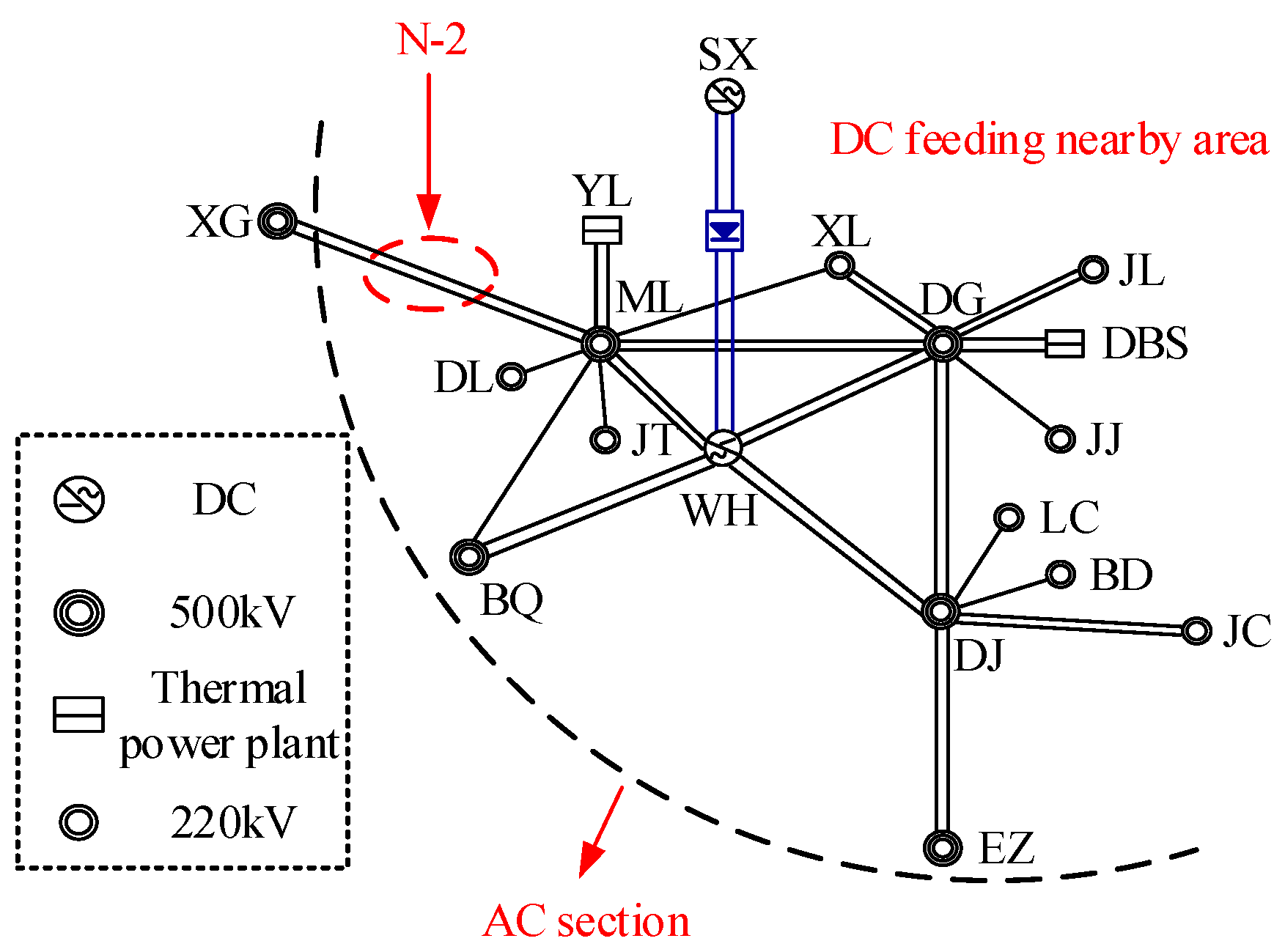
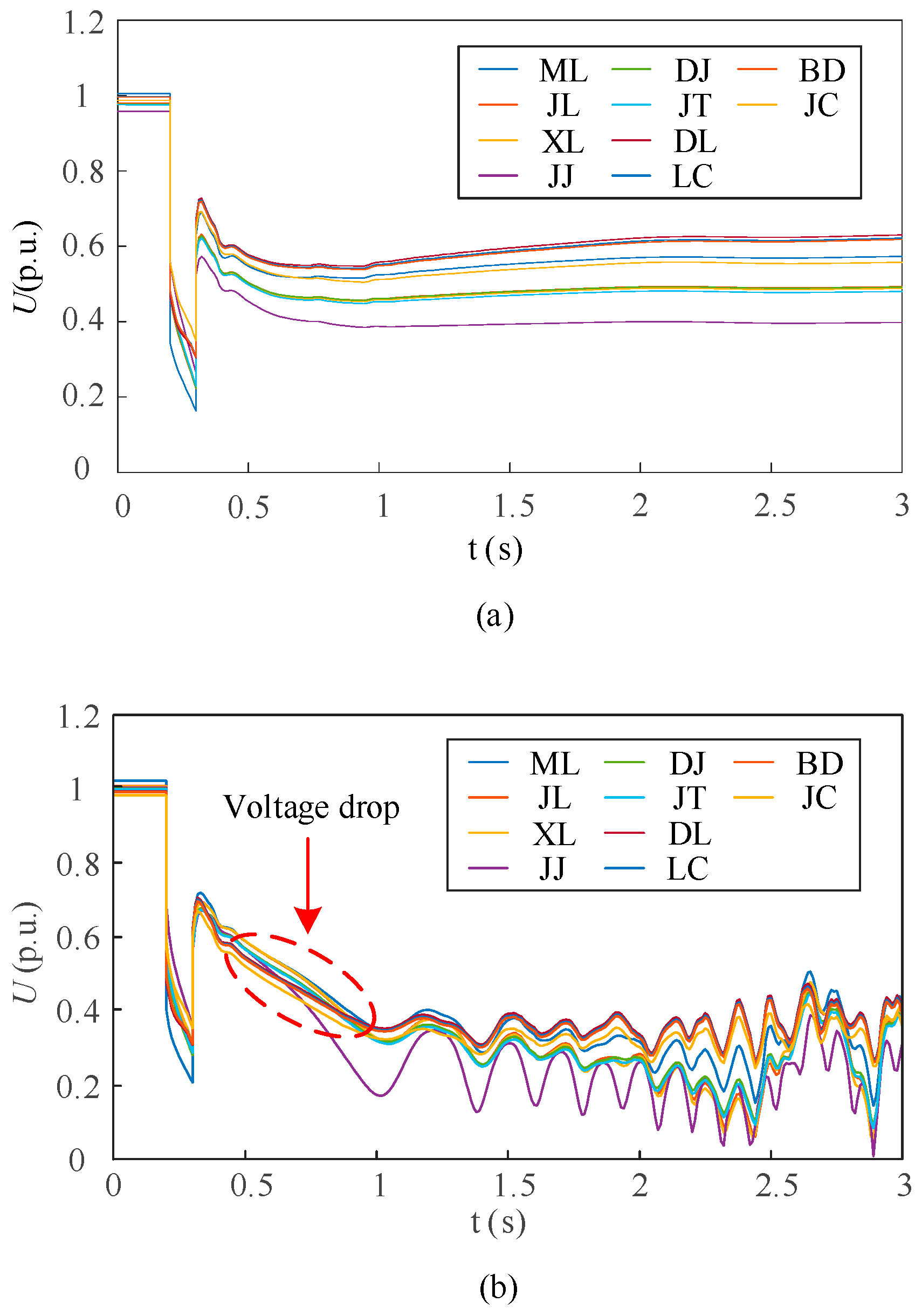
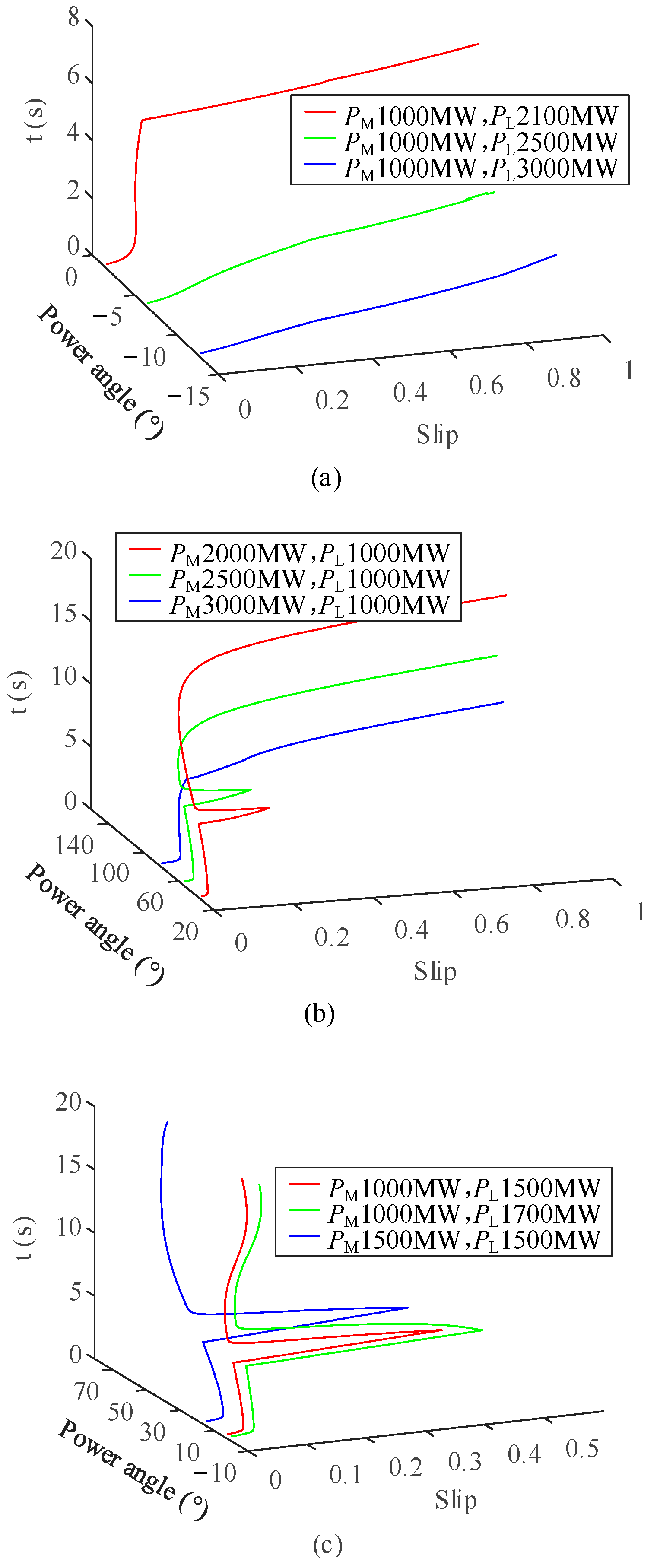
2.1. Voltage Instability Characteristics of SW DC Receiving-End Grid

Synchronous generators regulate excitation to maintain stable output voltage, thereby providing support for the system’s voltage stability. In practical operations, to ensure voltage stability, a minimum generators’ capacity is set for each region, and dispatch must strictly adhere to these requirements. However, in a simulation of a power grid in central China, it was found that increasing the generators’ capacity still led to system instability after a fault, making it impossible to identify a stable operating generators’ capacity range for the receiving-end grid. The structure of the grid is shown in Figure 1: the SW DC dropout point is the WH converter station, with four outgoing lines from the low-voltage side, respectively, connecting to BQ and DG; four outgoing lines from the high-voltage side connect to ML and DJ. YL and DBS are local generators, while XG, BQ, ML, DG, DJ, and EZ are 500 kV substations, and the remaining nodes are 220 kV substations.

A three-phase short-circuit fault is set on the line from ML to XG, and the faulted double circuit is disconnected after 100 ms, resulting in system voltage instability. The post-fault receiving-end voltage under the scenarios of both low and high generators’ capacity is shown in Figure 2a and Figure 2b, respectively. With a higher generators’ capacity, power angle instability occurs in generators such as YL and DBS after the fault, as shown in Figure 2c. Comparing the total system load curves under both generators’ capacity conditions in Figure 2d, it is evident that either too few or too many local generators’ capacity online leads to the failure of the load to recover after the fault.

Based on observed instability after faults in practical engineering, the relationship between generators’ capacity and receiving-end grid stability is established. As shown in Figure 3a, the red curve shows the voltage stability limit, and the blue curve shows the power angle limit. when the generators’ capacity is low, the system is limited by voltage instability; when capacity is high, it is constrained by power angle instability. These two factors together define the stable pre-control generators’ capacity range for the receiving-end grid. For grids with poor stability, as shown in Figure 3b, the minimum generators’ capacity constrained by voltage instability exceeds the maximum capacity constrained by power angle stability, resulting in no stable pre-control range. In such cases, reserve spinning capacity must be provided, and active power output constrained by power angle stability should be distributed across multiple generators to ensure both voltage and power angle stability. This paper primarily focuses on the upper limit of generators’ capacity under power angle stability, considering the interaction between DC power, load, and power angle swinging, and quantifying the generators’ capacity range.

2.2. The Coupling Characteristics Between Generators and Loads

First, the simplified system model shown in Figure 4 is established. In the figure, node 1, where the generator G is located, is connected to an infinite bus system through the reactance X_a and X_b, with U₁ ∠ $\delta$ representing the generator’s equivalent internal voltage. Node 2 represents the motor node, with voltage U₂ ∠ θ₂, while node 3 represents the infinite power source with voltage U_s ∠ 0.

The mathematical equations for the system shown in Figure 4 are as follows:

$$\left\{\begin{array}{c}{\displaystyle \frac{d\delta }{dt}}=(\omega -1){\omega }_0\hfill \\ {\displaystyle \frac{d\omega }{dt}}={\displaystyle \frac{1}{T_{\mathrm{J}}}}(P_{\mathrm{M}}-{\displaystyle \frac{U_1*U_2\sin (\delta -{\theta }_2)}{X_a}})\hfill \\ {\displaystyle \frac{ds}{dt}}={\displaystyle \frac{1}{T_{\mathrm{j}}}}(T_{\mathrm{m}}-T_{\mathrm{e}})\hfill \\ \begin{array}{l}{P}_2={\displaystyle \frac{U_1*U_2\sin (\delta -{\theta }_2)}{X_{\mathrm{a}}}}+{\displaystyle \frac{U_s{U}_2\sin (0-{\theta }_2)}{X_{\mathrm{b}}}}-{\displaystyle \frac{{U_2}^2}{R_{\mathrm{e}}}}\hfill \\ Q_2={\displaystyle \frac{U_1*U_2\cos (\delta -{\theta }_2)}{X_{\mathrm{a}}}}-{\displaystyle \frac{{U_2}^2}{X_{\mathrm{a}}}}+{\displaystyle \frac{U_s{U}_2\cos (0-{\theta }_2)}{X_{\mathrm{b}}}}-{\displaystyle \frac{{U_2}^2}{X_{\mathrm{b}}}}-{\displaystyle \frac{{U_2}^2}{X_{\mathrm{e}}}}\hfill \end{array}\hfill \end{array}\right.$$

(1)

In the equations, $\delta$ is the power angle of the synchronous machine, $\omega$ is the rotational speed, $s$ is the motor slip, T_J and T_j are the inertia time constants of the synchronous machine and the motor, respectively, ${\omega }_0$ is the synchronous speed of the synchronous machine, P_M is the mechanical power of the synchronous machine, T_m is the mechanical torque of the motor, P₂ and Q₂ are the active and reactive power transmitted to node 2, and Re and Xe are the equivalent resistance and reactance of the motor.

Based on the above mathematical model, the power angle and voltage instability characteristics can be analyzed. A direct ground fault is applied, and after 0.6 s, the fault is cleared, resulting in the power angle and slip trajectories under different generators’ capacity and load levels, as shown in Figure 5. In Figure 5a, when the local generators’ capacity is low, the system’s voltage support capability is weak, and the slip variation is large after the fault. As the load P_L increases, with a fixed generators’ capacity, the motor becomes unstable faster, while the local generator’s power angle oscillation is relatively small. In this case, load instability dominates the system’s in-stability. As shown in Figure 5b, with an increase in P_L, while keeping the generators’ capacity fixed, the power angle swings more significantly after the fault, and the load also becomes unstable. In Figure 5c, when both the generators’ capacity and load power are low, the system recovers stability. In summary, with changes in the ratio of generators and loads, the degree to which the power angle and load contribute to instability varies.

Given different initial values for the power angle and slip, the stable regions of the state variables can be plotted. Figure 6a shows the division of the stable region when the local generators’ capacity is 1500 MW and the load is 2500 MW, while Figure 6b shows the division of the stable region when the local generators’ capacity is 2500 MW and the load is 1500 MW. Comparing the two scenarios, when the load is high, the slip stability region is smaller, and the power angle stability region is larger, making the system more prone to voltage instability. On the other hand, when the local generators’ capacity is high, the power angle stability region is smaller, while the slip stability region is larger, making the system more prone to power angle instability. Within the stable region, even when the initial slip value is large, the system can still stabilize, indicating good voltage stability.

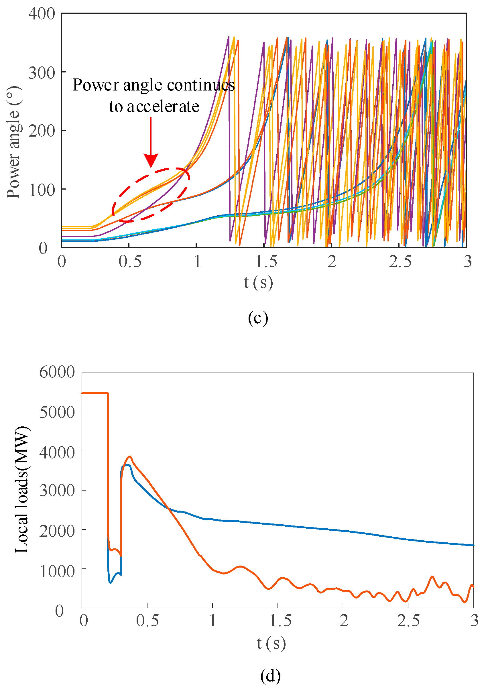
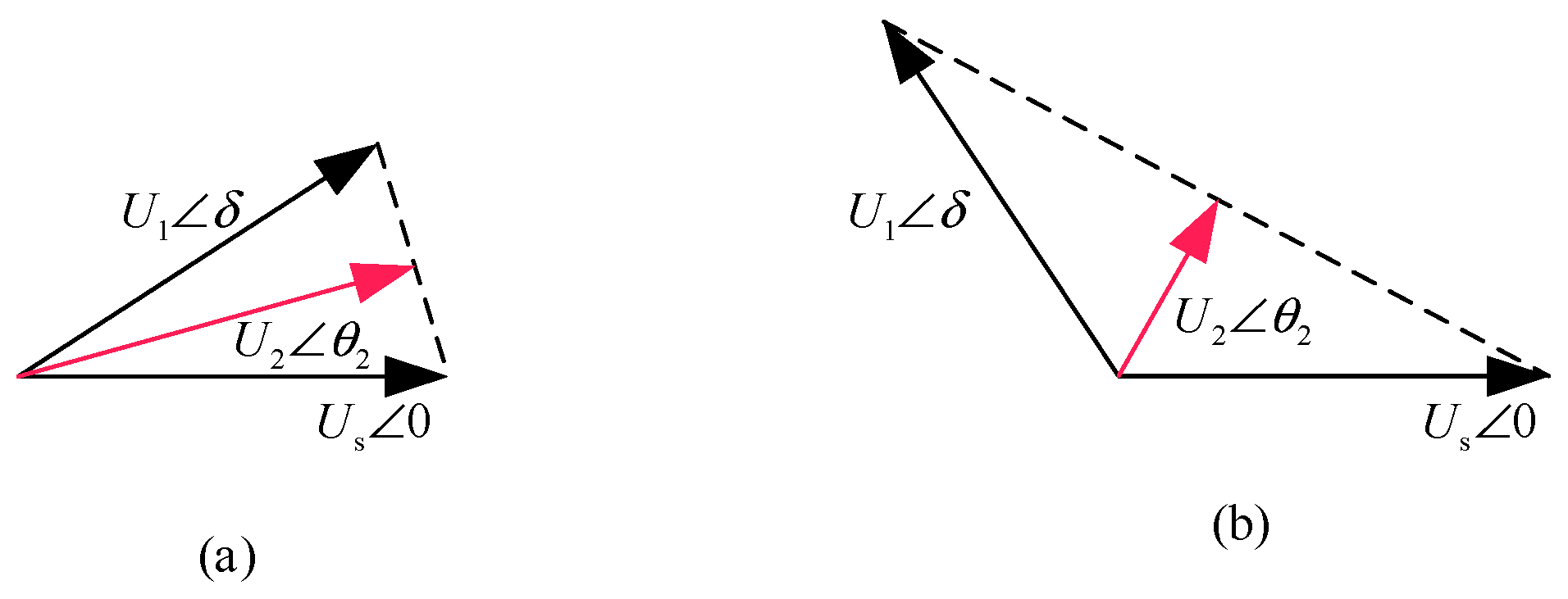
2.3. The Mechanism of Voltage Decline Due to Power Angle Swinging

When the power angle swings too far, it causes a voltage drop in the load. For the local generator and infinite power source, excluding the motor load, the Thevenin equivalent theorem is applied, with the equivalent voltage given by the following:

$$U_2\angle {\theta }_2={\displaystyle \frac{X_{\mathrm{b}}}{X_{\mathrm{a}}+X_{\mathrm{b}}}}{U}_1\angle \delta +{\displaystyle \frac{X_{\mathrm{a}}}{X_{\mathrm{a}}+X_{\mathrm{b}}}}{U}_{\mathrm{s}}\angle 0$$

(2)

When the power angle swings too far, it causes a voltage drop in the load. For the local generator and infinite power source, excluding the motor load, the Thevenin equivalent theorem is applied, with the equivalent voltage given by the following. From Equation (2), the relationship between the power angle and the equivalent voltage is derived, as shown in Figure 7. As the power angle difference increases, the magnitude of the equivalent voltage decreases, leading to a corresponding voltage drop at the load bus.

3. Stability Analysis of the AC/DC Receiving-End Grid

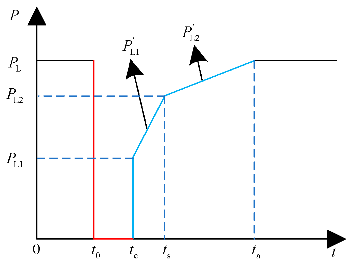
3.1. Load Recovery Characteristics

In practical power systems, the coupling effects among various dynamic components are significant, with the interaction between synchronous generators and induction motors being particularly complex. Since their state variables (power angle and slip) share similar dynamic time scales, achieving a fully decoupled analysis is challenging. Therefore, to study the post-fault recovery process of load and DC power, this paper employs a time-domain simulation trajectory fitting method, approximating their recovery characteristics as a linear process with a fixed slope. As shown in Figure 8, at the moment of fault clearing, the system voltage instantaneously recovers, and the load P_L also instantaneously recovers to P_L1. The recovery process of the load power P_L after fault clearing can be divided into two phases: the first phase considers the coupling effect between DC power and the load, corresponding to time t_c to t_s, while the second phase represents the recovery of the load alone after the DC power has returned to its initial value, which corresponds to time t_s to t_a.

The recovery rates of the load in the first and second phases can be approximately assumed to follow linear recovery with fixed slopes k₁ and k₂. Therefore, after fault clearing, the mathematical expression for the entire load power recovery process is given by Equation (3):

$$P_{\mathrm{L}}=\left\{\begin{array}{l}{P}_{\mathrm{L}}\hspace{1em}\hspace{1em}\hspace{1em}\hspace{1em}\hspace{1em}\hspace{1em}\hspace{1em}\hspace{1em}\hspace{1em} t<t_0\hfill \\ 0\hspace{1em}\hspace{1em}\hspace{1em}\hspace{1em}\hspace{1em}\hspace{1em}\hspace{1em}\hspace{1em}\hspace{1em} t_0<t<t_{\mathrm{c}}\hfill \\ P_{\mathrm{L}1}+P_{\mathrm{L}}ramp(k_1,t-t_{\mathrm{c}})\hspace{1em} t_{\mathrm{c}}<t<t_{\mathrm{s}}\hfill \\ P_{\mathrm{L}2}+P_{\mathrm{L}}ramp(k_2,t-t_{\mathrm{s}})\hspace{1em} t_{\mathrm{s}}<t<t_{\mathrm{a}}\hfill \end{array}\right.$$

(3)

In this equation, the parameters k₁ and k₂ in the function represent the recovery rates of the load power in the first and second phases, corresponding to the load recovery powers P′_L1 and P′_L2, respectively.

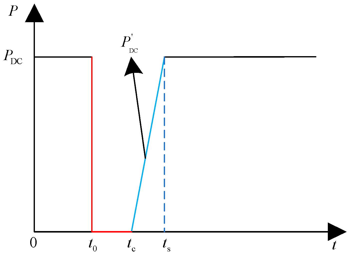
3.2. DC Power Recovery Characteristics

When an AC fault occurs in the system, the DC power decreases. When the fault is serious, the power drops to 0, After the fault is cleared, the DC power enters the recovery phase under the control system’s regulation, corresponding to time t_c to t_s. The dynamic adjustment process of DC power is very fast, with the recovery to the initial power state taking approximately a hundred milliseconds after the fault clearing. The DC power recovery characteristic curve is shown in Figure 9.

Based on the above analysis, the power variation during the DC recovery process can be reflected by the main characteristic points and the times at which these points occur, leading to the establishment of a DC power recovery time characteristic model [34]. The mathematical expression for the entire DC power recovery process is given by Equation (4):

$$P_{\mathrm{DC}}=\left\{\begin{array}{l}{P}_{\mathrm{DC}}\hspace{1em}\hspace{1em}\hspace{1em}\hspace{1em}\hspace{1em}\hspace{1em}\hspace{1em}t<t_0\hfill \\ 0\hspace{1em}\hspace{1em}\hspace{1em}\hspace{1em}\hspace{1em}\hspace{1em}\hspace{1em} t_0<t<t_{\mathrm{c}}\hfill \\ P_{\mathrm{DC}}ramp(k_3,t-t_{\mathrm{c}})\hspace{1em} t_{\mathrm{c}}<t<t_{\mathrm{s}}\hfill \end{array}\right.$$

(4)

In this equation, the parameter k₃ in the function represents the recovery rate of the DC line power, corresponding to the DC recovery power P′_DC.

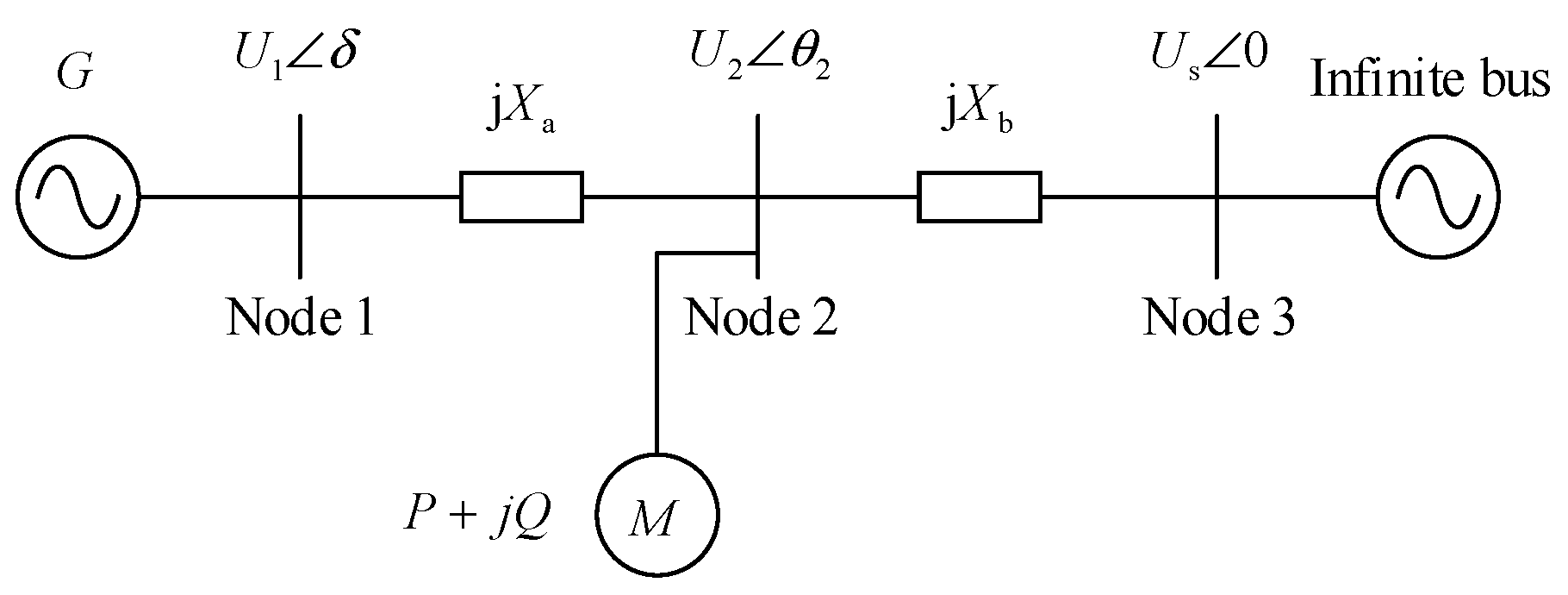
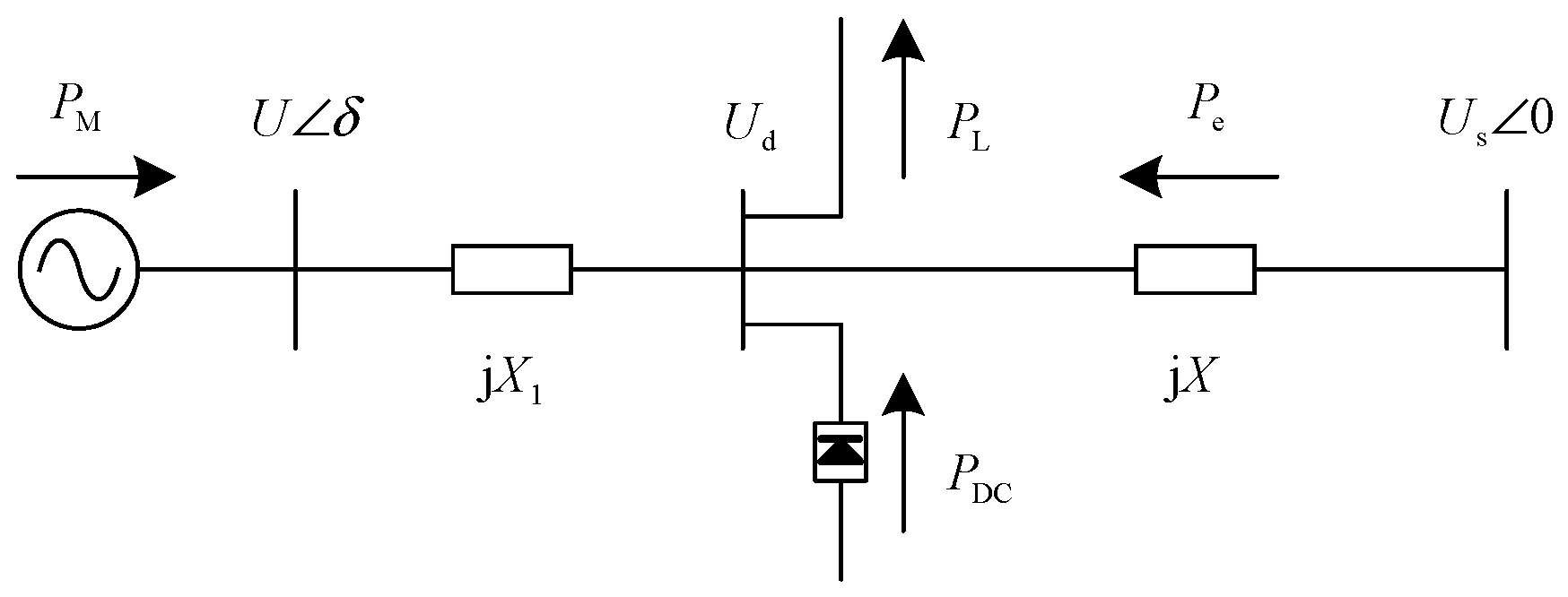
3.3. The Simplified Model of the Receiving-End Grid and Stability Analysis

Based on the actual AC/DC hybrid grid structure at the receiving end, the simplified model of the receiving-end system is constructed as shown in Figure 10. In the figure, U ∠ $\delta$ represents the internal voltage of the local generator, U_d is the equivalent voltage at the DC connection point, U_s ∠ 0 is the voltage of the infinite bus, P_M denotes the active power output of the local generator, P_e represents the power transmitted from the external grid to the receiving end (with positive flow indicating power transmitted from the receiving end to the external grid), P_DC is the DC power, P_L is the load power, and X, X₁ represents the equivalent reactance between each node. Considering the tight interconnection of the receiving-end grid, X₁ is neglected in the calculation.

The second-order rotor motion equation for the simplified system is as follows:

$${\displaystyle \frac{d^2\delta }{d{t}^2}}={\displaystyle \frac{1}{T_{\mathrm{J}}}}(P_{\mathrm{M}}+P_{\mathrm{DC}}-P_{\mathrm{L}}-{\displaystyle \frac{U\times U_{\mathrm{s}}}{X}}\sin \delta )$$

(5)

For the simplified AC/DC receiving-end grid model shown in Figure 10, when a three-phase short circuit occurs in the nearby AC system, the power–power angle curve shown in Figure 11 can be derived based on Equation (5). At the corresponding moment ${\delta }_0$ of t₀, a three-phase short circuit occurs at the receiving end. Considering the worst-case scenario, the DC power P_DC drops instantaneously to 0, the electromagnetic power shifts from P_e to P′_e = 0, and the electromagnetic power operating point moves from a to b. During the fault, the system’s electromagnetic power operating point shifts along P′_e = 0 and moves to the right to c. At the corresponding moment t_c, the fault is cleared, and the electromagnetic power recovers from P′_e = 0 to P_e (assuming no topology changes), with the electromagnetic power operating point moving from c to d, and continuing to move along P_e toward the critical point e.

For other power conditions, the dynamic process from the fault clearance to the system’s recovery to a steady state can be divided into three stages:

(1)

The first stage corresponds to the period from time t_c to time t_s, during which the DC power and load power are in their first phase of recovery. The equivalent mechanical power during this stage is denoted as P_M + P′_DC − P′_L1;

(2)

The second stage corresponds to the period from time t_s to time t_a, after the DC power has been restored, during which the load power undergoes its second phase of recovery. The equivalent mechanical power during this stage is denoted as P_M + P_DC − P′_L2;

(3)

The third stage corresponds to the period from time t_a to time t_m, after both DC power and load power have been restored to their initial values. During this stage, the power angle continues to swing to its maximum value. The equivalent mechanical power during this stage is denoted as P_M + P_DC − P_L.

The transient stability characteristics of the system’s receiving end are influenced by factors such as local generators, DC power, and external AC power intake. The analysis is as follows:

(1)

DC and Local Generators Distribution

Increasing the DC power to replace local generators reduces the system’s acceleration area during a fault. A lower number of local generators leads to decreased volt-age support capability after the fault, slowing down the recovery of DC power and load, and reducing the system’s deceleration area. Therefore, the relationship between local generators and transient stability is not monotonic and should be analyzed based on the specific scenario.

(2)

AC/DC Power Distribution

Increasing the DC power to replace external AC intake, while assuming that both DC power and load are zero during the fault, leaves the system’s acceleration area unchanged during the fault. However, as the DC power increases, the generator operating point rises, reducing the system’s deceleration area and lowering its stability.

(3)

Local Generators and External AC Intake Distribution

Replacing external AC power with local generators increases the system’s acceleration area during a fault. However, as local generators increase, the recovery of load and DC power speeds up, resulting in an uncertain change in the deceleration area, which is also dependent on the location of the generators. Therefore, considering the overall changes in acceleration and deceleration areas, the stability change is uncertain.

4. Quantitative Analysis of Generators’ Capacity Range Under Transient Stability Constraints

Considering the power recovery characteristics of load and DC, based on Equation (5), the initial generator’s power angle before the fault can be expressed as follows:

$${\delta }_0=\arcsin ({\displaystyle \frac{P_{\mathrm{M}}+P_{\mathrm{DC}}-P_{\mathrm{L}}}{P}})$$

(6)

In this equation, $P=U\times U_s/X$ represent the static power angle stability limit power. Assuming that during the fault, P_e, P_DC, and P_L are all zero, the system’s rotor motion equation is as follows:

$$T_{\mathrm{J}}{\displaystyle \frac{d^2\delta }{d{t}^2}}=P_{\mathrm{M}}$$

(7)

For the fault clearance and recovery process, the power angle can be solved in three steps:

(1)

First, write the rotor motion equations for different stages;

(2)

Second, integrate to determine the generator’s speed;

(3)

Third, integrate to determine the power angle.

The solution steps are as follows:

At the moment of fault clearance, the generator’s speed ${\omega }_{\mathrm{c}}$ and power angle ${\delta }_{\mathrm{c}}$ are as follows:

$$\left\{\begin{array}{l}\omega (t_{\mathrm{c}})=\omega (0)+{\displaystyle {\int }_0^t\frac{P_{\mathrm{M}}}{T_{\mathrm{J}}}}d\tau \hfill \\ \delta (t_{\mathrm{c}})={\delta }_0+{\displaystyle {\int }_0^t{\omega }_0[\omega (\tau )-1]}d\tau \hfill \end{array}\right.$$

(8)

where $\omega (0)$ is the initial speed, and the per unit value is 1.

In the first stage, the DC power changes from P_DC to P′_DC, and the load power changes from P_L2 to P′_L1. The rotor motion equation for this stage is as follows:

$$T_{\mathrm{J}}{\displaystyle \frac{d^2\delta }{d{t}^2}}=(P_{\mathrm{M}}+P_{\mathrm{DC}}^{\prime }-P_{\mathrm{L}1}^{\prime })-P\sin \delta$$

(9)

At the end of the first stage recovery t_s, the generator’s speed ${\omega }_{\mathrm{s}}$ and power angle ${\delta }_{\mathrm{s}}$ are as follows:

$$\left\{\begin{array}{l}\omega (t_{\mathrm{s}})=\omega (t_{\mathrm{c}})+{\displaystyle {\int }_0^t\frac{P_{\mathrm{M}}+P_{\mathrm{DC}}^{\prime }-P_{\mathrm{L}1}^{\prime }-P\sin \delta }{T_{\mathrm{J}}}}d\tau \hfill \\ \delta (t_{\mathrm{s}})=\delta (t_{\mathrm{c}})+{\displaystyle {\int }_0^t{\omega }_{\mathrm{c}}[\omega (\tau )-1]}d\tau \hfill \end{array}\right.$$

(10)

In the second stage, the DC power has recovered to its initial state and the load power changes from P′_L1 to P′_L2. The rotor motion equation for this stage is as follows:

$$T_{\mathrm{J}}{\displaystyle \frac{d^2\delta }{d{t}^2}}=(P_{\mathrm{M}}+P_{\mathrm{DC}}-P_{\mathrm{L}2}^{\prime })-P\sin \delta$$

(11)

Similarly, at the end of the second stage recovery t_a, the generator’s speed ${\omega }_{\mathrm{a}}$ and power angle ${\delta }_{\mathrm{a}}$ are as follows:

$$\left\{\begin{array}{l}\omega (t_{\mathrm{a}})=\omega (t_{\mathrm{s}})+{\displaystyle {\int }_0^t\frac{P_{\mathrm{M}}+P_{\mathrm{DC}}-P_{\mathrm{L}2}^{\prime }-P\sin \delta }{T_{\mathrm{J}}}}d\tau \hfill \\ \delta (t_{\mathrm{a}})=\delta (t_{\mathrm{s}})+{\displaystyle {\int }_0^t{\omega }_{\mathrm{s}}[\omega (\tau )-1]}d\tau \hfill \end{array}\right.$$

(12)

After fault clearance, the maximum swing angle of the system is as follows:

$${\delta }_{\max }=\pi -{\delta }_0$$

(13)

As shown in Figure 11, the system’s acceleration area during the fault is as follows:

$$S={\displaystyle {\int }_{{\delta }_0}^{{\delta }_{\mathrm{c}}}{P}_{\mathrm{M}}}d\delta$$

(14)

After fault clearance, the system’s maximum deceleration area corresponds to the accumulated deceleration area during the three stages. The deceleration area for the first stage is as follows:

$$S_1={\displaystyle {\int }_{{\delta }_{\mathrm{c}}}^{{\delta }_{\mathrm{s}}}{P}_{\mathrm{L}1}^{\prime }+P\sin \delta -P_{\mathrm{DC}}^{\prime }-P_{\mathrm{M}}}d\delta$$

(15)

For the second and third stages, the deceleration areas of the system are calculated as per Equation (15). To maintain transient stability, the system’s accumulated acceleration area should be smaller than the deceleration area:

$$S<S_1+S_2+S_3$$

(16)

Based on the above equation, the local generators’ capacity range that satisfies the system’s power angle stability can be determined as follows:

$$\begin{array}{cc}\hfill P_{\mathrm{M}}<& {\displaystyle \frac{P(\cos {\delta }_{\mathrm{c}}-\cos {\delta }_{\max })+(P_{\mathrm{DC}}^{\prime }-P_{\mathrm{L}1}^{\prime }){\delta }_{\mathrm{c}}}{{\delta }_{\max }-{\delta }_0}}+\hfill \\ & {\displaystyle \frac{(P_{\mathrm{L}1}^{\prime }-P_{\mathrm{DC}}^{\prime }-P_{\mathrm{L}2}^{\prime }+P_{\mathrm{DC}}){\delta }_{\mathrm{s}}+}{{\delta }_{\max }-{\delta }_0}}+\hfill \\ & {\displaystyle \frac{(P_{\mathrm{L}}-P_{\mathrm{DC}}){\delta }_{\max }+(P_{\mathrm{L}2}^{\prime }-P_{\mathrm{L}}){\delta }_{\mathrm{a}}}{{\delta }_{\max }-{\delta }_0}}\hfill \end{array}$$

(17)

5. Case Verification

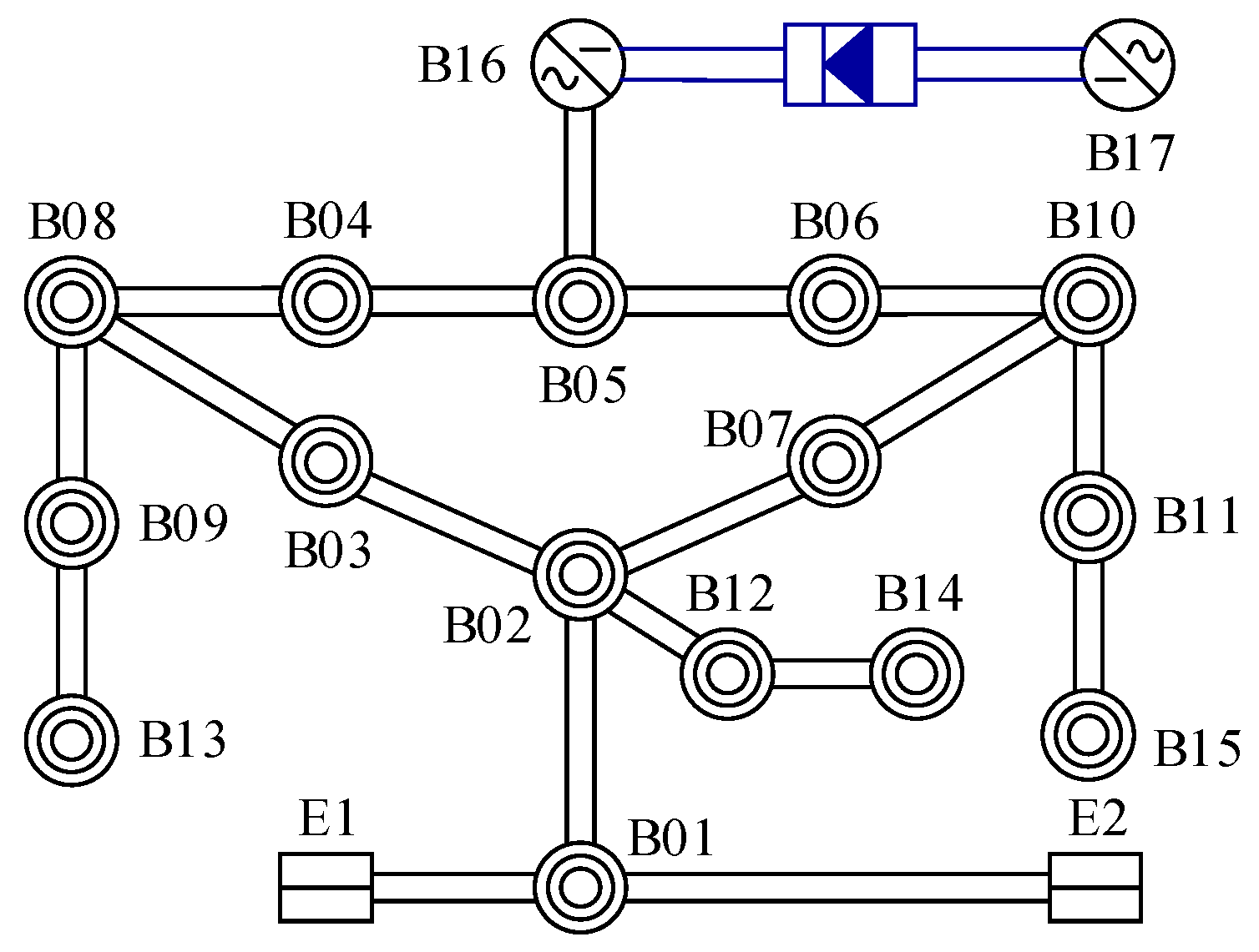
5.1. System Network Structure

The structure of a simplified actual power grid example is shown in Figure 12. The simplified example is obtained by equivalent aggregation of Figure 1. E1 represents the local generators at the AC-DC grid receiving end, while E2 represents the external AC grid, connected to the local grid via an AC transmission line. B02–B12 are the interconnection nodes at the receiving end, B13–B15 are the load nodes at the receiving end, and B16 and B17 are the DC nodes. The simulation software used in this paper is PSD-BPA developed by China Electric Power Academy of Sciences. A three-phase short-circuit fault is applied at the B05 side of the double-circuit line B04–B05 at 0.1 s, and the fault is cleared after 100 ms. Since the impact of system damping is minimal, it is therefore neglected. The reactance of the B01–B02 line is 0.012 p.u. The reactance of the B09–B13, B11–B15, and B12–B14 lines is 0.0125 p.u. The reactance of all other lines is 0.0005 p.u.

5.2. Sensitivity Factor Analysis of Transient Stability

5.2.1. DC and Local Generators Distribution

Keeping the total DC power and local generators’ capacity unchanged, as shown in Figure 13, an increase in DC power results in a reduction in the local generator’s power angle oscillation amplitude after a fault, thereby improving the system’s transient stability. However, as local generators decrease, the system’s voltage support capability is weakened, worsening the voltage stability. When the DC power becomes excessively large, the system becomes unstable after the fault, as illustrated in Figure 14.

5.2.2. AC/DC Power Distribution

Keeping the total AC transmission power and DC power unchanged, as shown in Figure 15, an increase in DC power leads to a continuous increase in the local generator’s power angle oscillation amplitude after a fault, resulting in a reduction in the system’s transient stability. When the DC power reaches a certain threshold, the system becomes unstable after the fault.

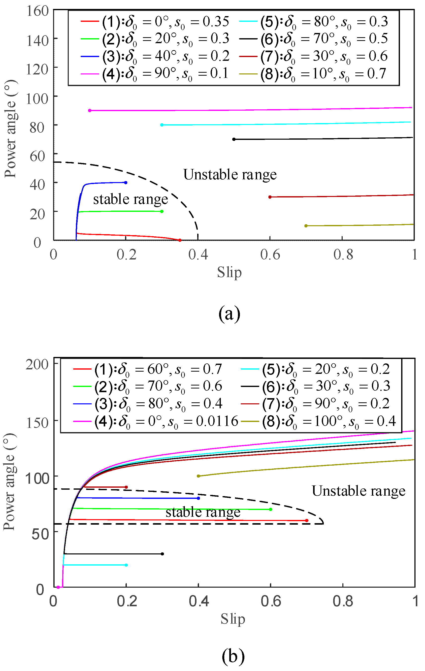
5.2.3. Static Power Angle Stability Limit

Keeping the DC power, local generators’ capacity, and load unchanged, while adjusting the transmission line impedance, changes the system’s static power angle stability limit P. As the static power angle stability limit increases, as shown in Figure 16, the oscillation amplitude of the local generator’s power angle gradually decreases after the fault. Additionally, the system voltage recovers more quickly post-fault, leading to an overall improvement in the system’s transient stability.

5.3. Simulation Verification of Local Generators’ Capacity Range

Simulation calculations were performed on the power grid example shown in Figure 12 under different operating conditions to validate the calculation method for the maximum generators’ capacity. The results of the actual grid time-domain simulation and the calculation results using the method proposed in this paper are shown in

Table 1. Local generators’ capacity range under transient power angle stability constraints.

Different Operating Conditions	Simulation Value	Theoretical Value	Error (%)
DC power 800 MW, Load 2400 MW;	1895	2030	7.12
DC power 1000 MW, Load 2600 MW;	1925	2114	9.82
DC power 1200 MW, Load 2800 MW;	1980	2183	10.25
DC power 1000 MW, Load 2400 MW;	1725	1830	6.09
DC power 1200 MW, Load 2400 MW;	1595	1650	3.45

. The error between the proposed method and the time-domain simulation results does not exceed 10.25%, demonstrating that the proposed method for quantifying the maximum generators’ capacity has good accuracy.

6. Conclusions

This study conducts an in-depth analysis of the coupling mechanism between power angle stability and voltage stability. For the first time, it quantitatively characterizes the stable operating region of the system using power angle and induction motor slip as dual constraint conditions, providing a new theoretical framework for power system stability analysis. Additionally, addressing the lack of quantitative research on the upper limit of generator operation in current systems, this study constructs post-fault power recovery curves for loads and DC power sources. The main conclusions are as follows:

(1)

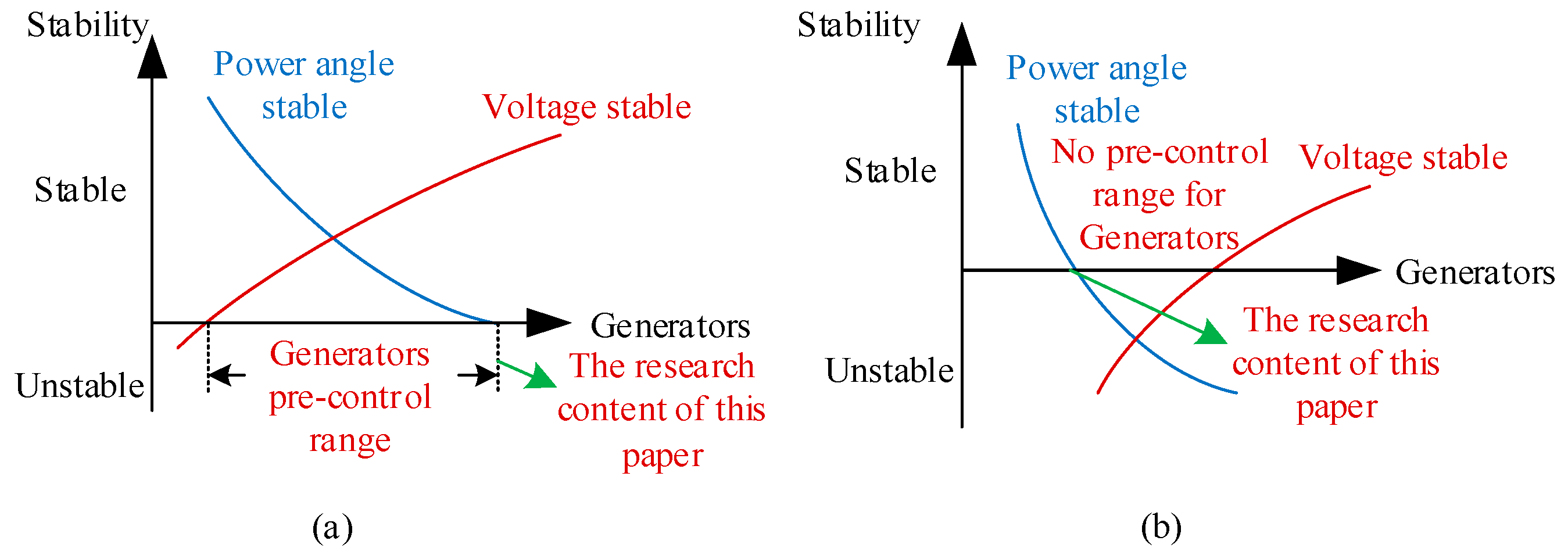
Increasing the number of local generators’ capacity is an effective measure to address voltage stability issues. However, excessive generators’ capacity can lead to power angle stability problems, resulting in some receiving end grids lacking a stable generators’ capacity pre-control range. Therefore, the generators’ capacity for receiving end grids should be limited;

(2)

As the number of local generators’ capacity increases, the grid transitions from a voltage stability issue to a power angle stability issue. A higher number of local generators’ capacity leads to larger power angle swings after faults, which in turn reduces the Thevenin equivalent voltage seen by the load, exacerbating the system voltage drop. In practical power systems, if other factors are not considered, the transition between voltage stability and power angle stability primarily depends on the proportional relationship between the generators’ capacity level and the load level. Traditional stability assessment methods typically analyze the system based on a single constraint condition (either voltage or power angle), without explicitly defining the reasonable range of generators’ capacity or quantifying the induction motor load capacity that the system can withstand. This limitation makes it difficult for existing methods to fully capture the actual stability characteristics of the system;

(3)

In the allocation of DC power, local generators, and AC power replacement, the system stability does not change monotonically, and a specific grid analysis is needed;

(4)

Considering the two-phase recovery characteristics of DC power and load after a fault, this paper proposes a method for quantifying the maximum generators’ capacity limit, with a calculation error not exceeding 10.25%. Within the calculated range, the generators’ capacity can ensure that the receiving end system does not become unstable due to excessive power angle acceleration.

This paper provides a quantitative study on the instability caused by excessive generators’ capacity leading to loss of synchronism. However, further analysis is needed for the quantification of minimum generators’ capacity limits under voltage instability constraints. Additionally, for situations where no stable generators’ capacity pre-control range exists, further research is required on how to maintain a spinning reserve.

References

1. Dong, X.; Tang, Y.; Bu, G. Confronting Problem and Challenge of Large Scale AC-DC Hybrid Power Grid Operation. Proc. CSEE 2019, 39, 3107–3119. [Google Scholar]
2. Zhou, X.; Chen, S.; Lu, Z. Technology Features of the New Generation Power System in China. Proc. CSEE 2018, 38, 1893–1904. [Google Scholar]
3. Tang, Y. Voltage Stability Analysis of Power System; Beijing Science Press: Beijing, China, 2011. [Google Scholar]
4. Kawabe, K.; Tanaka, K. Analytical Method for Short-Term Voltage Stability Using the Stability Boundary in the P-V Plane. IEEE Trans. Power Syst. 2014, 29, 3041–3047. [Google Scholar] [CrossRef]
5. Sun, H.; Zhou, X.; Li, R. Influence of Induction Motor Load Parameters on Power System Transient Voltage Stability. Power Syst. Technol. 2005, 29, 1–6. [Google Scholar]
6. Li, L.; Lu, C.; Huang, Z. Analytical Assessment of Transient Voltage Stability of Load Bus Considering Induction Motors. Autom. Electr. Power Syst. 2009, 33, 1–5. [Google Scholar]
7. He, L.; Li, X.; Xu, M. Assessment of Ransient Voltage Stability of Load Bus Considering the Mechanical Torque of Dynamic Load. Autom. Electr. Power Syst. 2010, 34, 1–5. [Google Scholar]
8. Zhang, W.; Zhang, B.; Pan, J. Mechanism Analysis for Transient Voltage Instability Based on Crossfeed Characteristics between Power Network and Load of Induction Motor. Autom. Electr. Power Syst. 2017, 41, 8–14. [Google Scholar]
9. Du, W.; Su, G.; Wang, H.; Ji, Y. Dynamic Instability of a Power System Caused by Aggregation of Induction Motor Loads. IEEE Trans. Power Syst. 2019, 34, 4361–4369. [Google Scholar] [CrossRef]
10. Yao, R.; Sun, K.; Shi, D.; Zhang, X. Voltage Stability Analysis of Power Systems with Induction Motors Based on Holomorphic Embedding. IEEE Trans. Power Syst. 2019, 34, 1278–1288. [Google Scholar] [CrossRef]
11. Aik, D.L.H.; Andersson, G. Power stability analysis of multi-infeed HVDC systems. IEEE Trans. Power Deliv. 1998, 13, 923–931. [Google Scholar] [CrossRef]
12. Zhang, F.; Xin, H.-H.; Xu, Q.; Dai, P.; Qin, X.-H. Generalized Short Circuit Ratio for Multi-infeed DC Systems: Influence Factors. Proc. CSEE 2017, 37, 5303–5312. [Google Scholar]
13. Xiao, H.; Li, Y.; Shi, D. Integrated Short Circuit Ratio Strength Index for Static Voltage Stability analysis of Multi-infeed LCC-HVDC Systems. Proc. CSEE 2017, 37, 6471–6480. [Google Scholar]
14. Li, D.; Sun, M.; Zhao, Y. The Steady-state Voltage Stability Analysis of Multi-infeed LCC-HVDC System Based on Equivalent Operating Short Circuit Ratio. Proc. CSEE 2020, 40, 3847–3857. [Google Scholar]
15. Qiu, W.; He, J.; Yu, Z. Transient Voltage Stability Analysis of Hunan Power Grid with Infeed UHVDC. Electr. Power Autom. Equip. 2019, 39, 168–173. [Google Scholar]
16. Bian, H.; Pan, X.; Liu, F. Study on Voltage Stability Analysis and Improvement Measures for Henan Province with a Background of Multiple DC Feeding. Power Syst. Prot. Control 2020, 48, 125–131. [Google Scholar]
17. Ran, H.; Wang, Z.; Gao, B. Two-stage Transient Voltage Evaluation Suitable for HVDC Receiving Systems. Power Syst. Technol. 2023, 47, 4272–4284. [Google Scholar]
18. Zhang, Q.; Feng, Y.; Cui, Y. Overall consideration of peak regulation and voltage stability on scheduling units in Shanghai power grid with multiple HVDC feed-in. Power Syst. Clean Energy 2016, 32, 54–60. [Google Scholar]
19. Wang, E.; Liu, H.; Chen, R. Comparative Analysis of Near-Zone Characteristics of Shan-Wu DC Based on Jing-Wu Double Circuit Constraint Fault. Hubei Electr. Power 2022, 46, 42–50. [Google Scholar]
20. Deng, H.; Lou, B.; Hua, W. Study on AC/DC hybrid characteristics and generator set optimization in Zhejiang power grid. Shaanxi Electr. Power 2017, 45, 55–59. [Google Scholar]
21. Liu, Y.; Li, Z.; Zhang, Z. An Analytical Calculation Method for Total Transfer Capability of Transmission Section Based on Evaluation of System Short Circuit Capability. Electr. Power 2025, 58, 98–107. [Google Scholar]
22. Qin, J.; Li, H.; Sun, Y. Optimization method for minimum start-up mode of conventional units considering constraints on the maximum grid connection strength of new energy. Power Syst. Prot. Control 2023, 51, 127–135. [Google Scholar]
23. Yao, J.; Chen, Z.; Zhang, W. Minimum Start-up Sequence Method of Receiving Terminal Based on Generator and Load Dynamic Reactive Power Response. Smart Power 2018, 46, 66–71. [Google Scholar]
24. Bian, H.; Wang, K.; Huang, C. Analysis of Key Indicators for Transient Voltage Recovery and Their Application in DC Receiving-End Systems. Jiangxi Electr. Power 2022, 46, 17–20+24. [Google Scholar]
25. Jia, Q.; Peng, L.; Wang, X. Method for Determining the Minimum Capacity Scale of Generators Under Voltage Stability Constraints. In Proceedings of the 2023 IEEE International Conference on Advanced Power System Automation and Protection (APAP), Xuchang, China, 8–12 October 2023; pp. 119–123. [Google Scholar]
26. Van Cutsem, T.; Vouras, C.D. Voltage stability analysis in transient and mid-termtime scales. IEEE Trans. Power Syst. 1996, 11, 146–154. [Google Scholar] [CrossRef]
27. Wei, W.; Yong, T.; Huadong, S.; Jian, H.; Weifang, L. The Recognition of Principal Mode between Rotor Angle Instability and Transient Voltage Instability. Proc. CSEE 2014, 34, 5610–5617. [Google Scholar]
28. Zheng, C.; Sun, H.; Zhang, A.; Lv, S. Discrimination of Rotor Angle Stability and Voltage Stability Based on Wide-area Branch Response and Emergency Control. Proc. CSEE 2021, 41, 6148–6160. [Google Scholar]
29. Gu, Z.; Tang, Y.; Yi, J. Study on Mechanism of Interrelationship between Power System Angle Stability and Induction Motor Stability. Power Syst. Technol. 2017, 41, 2499–2505. [Google Scholar]
30. Li, X.; Liu, C.; Xin, S. Coupling Mechanism Analysis and Coupling Strength Evaluation Index of Transient Power Angle Stability and Transient Voltage Stability. Proc. CSEE 2021, 41, 5091–5107. [Google Scholar]
31. Shi, Z.; Yao, W.; Huang, Y. Power System Dominant Instability Mode Identification Based on Convolutional Neural Networks with Squeeze and Excitation Block and Simulation Data. Proc. CSEE 2022, 42, 7719–7731. [Google Scholar]
32. Zhang, R.; Yao, W.; Shi, Z. Semi-supervised Learning Framework of Dominant Instability Mode Identification Via Fusion of Virtual Adversarial Training and Mean Teacher Model. Proc. CSEE 2022, 42, 7497–7509. [Google Scholar]
33. Vournas, C.D.; Sauer, P.W.; Pai, M.A. Relationships between voltage and angle stability of power systems. Int. J. Electr. Power Energy Syst. 1996, 18, 493–500. [Google Scholar] [CrossRef]
34. Wang, Z.; Hu, J.; Wang, T. Analysis of Impact of Power Recovery Speed on Transient Stability of Sending-side System after Large Capacity HVDC Commutation Failure. Power Syst. Technol. 2020, 44, 1815–1825. [Google Scholar]
Figure 1. SW DC feeding system structure for the nearby area.
Energies 18 01925 g001
Figure 2. Local generator power angle, system voltage, and local load curve. (a) System voltage curve with a low number of local generators. (b) System voltage curve with a low number of local generators. (c) Power angle curves of local generators with a high number of local generators. (d) Comparison of load power under different local generator levels.
Energies 18 01925 g002aEnergies 18 01925 g002b
Figure 3. Stability characteristics of receiving-end systems under different generators’ pre-control range. (a) Stability characteristics of receiving-end systems with generators’ pre-control range. (b) Stability characteristics of receiving-end systems without generators’ pre-control range.
Energies 18 01925 g003
Figure 4. Simplified model of system.
Energies 18 01925 g004
Figure 5. Power angle and slip variation curves over time under different cases of PM and PL. (a) Fixed PM, only changed PL. (b) Fixed PM, only changed PL. (c) Fixed PM, only changed PL.
Energies 18 01925 g005
Figure 6. System stability region under dual constraints of power angle and slip. (a) Dynamic relationship between power angle and slip under heavy load. (b) Dynamic relationship between power angle and slip under more generators.
Energies 18 01925 g006
Figure 7. Relationship between power angle and system equivalent voltage. (a) Equivalent voltage in stable conditions. (b) Equivalent voltage when the power angle swings too quickly.
Energies 18 01925 g007
Figure 8. Load power recovery characteristic curve.
Energies 18 01925 g008
Figure 9. DC power recovery characteristic curve.
Energies 18 01925 g009
Figure 10. Simplified mathematical model of receiver system.
Energies 18 01925 g010
Figure 11. Power-angle characteristic curve of the generator under AC fault.
Energies 18 01925 g011
Figure 12. Simplified power grid example PSD-BPA diagram.
Energies 18 01925 g012
Figure 13. Local generators’ power angle and system voltage under different DC and local generators distribution. (a) local generators’ power angle. (b) system voltage.
Energies 18 01925 g013
Figure 14. Local generators’ power angle and bus voltage with unchanged DC and local generators distribution, when DC power is 1800 MW. (a) local generators’ power angle. (b) system voltage.
Energies 18 01925 g014
Figure 15. Local generators’ power angle and system voltage under different AC/DC power distribution. (a) local generators’ power angle. (b) system voltage.
Energies 18 01925 g015
Figure 16. Local generators’ power angle and system voltage under different static power angle stability limit. (a) local generators’ power angle. (b) system voltage.
Energies 18 01925 g016