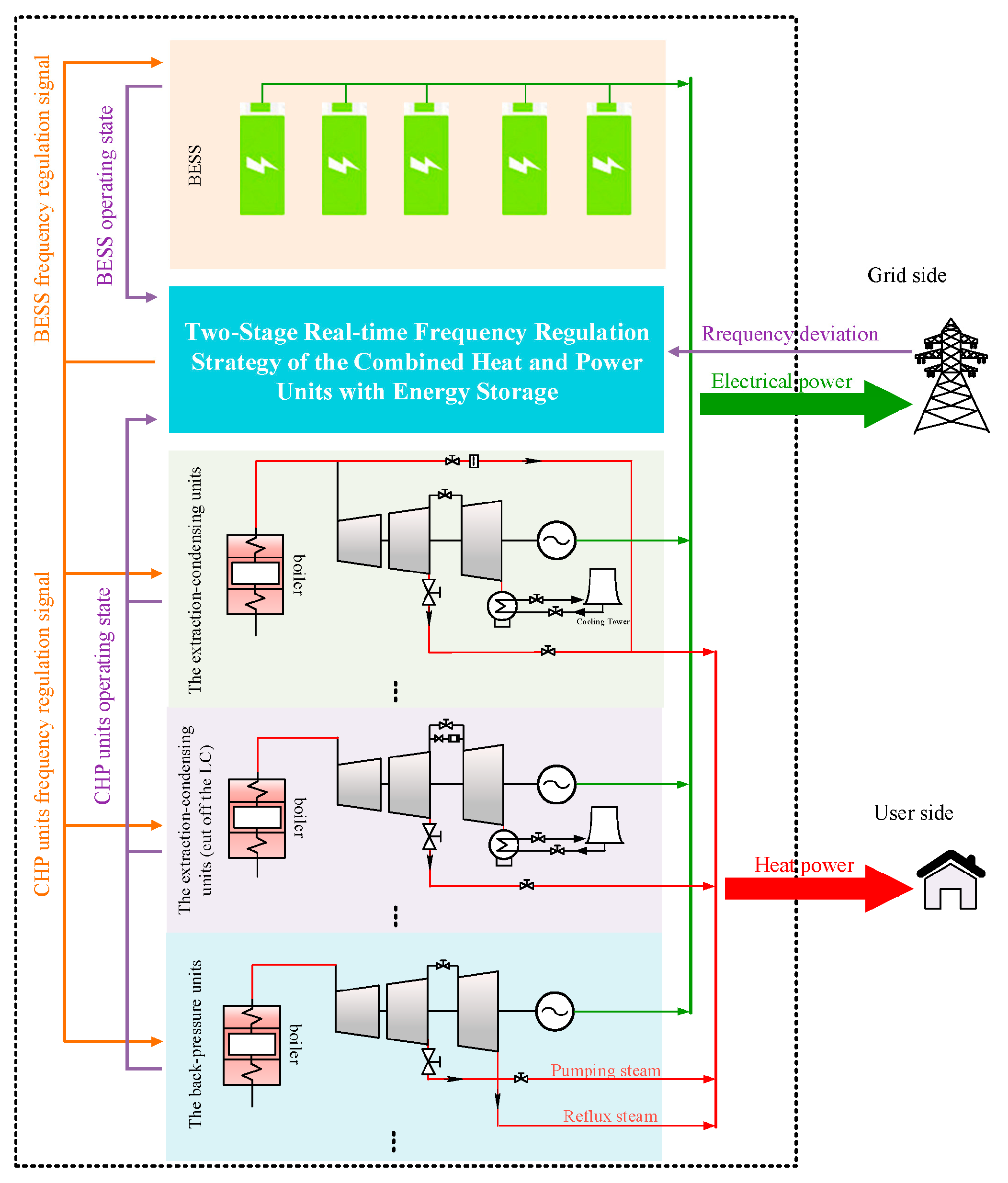
Two-Stage Real-Time Frequency Regulation Strategy of Combined Heat and Power Units with Energy Storage

Abstract

In view of the frequency regulation (FR) policy in Northeast China, a two-stage real-time rolling optimization model for power plants participating in FR ancillary services is established. The optimization object of the first stage is to maximize the overall profitability of the power plant and to obtain FR performance sub-indicators (K₁, K₂, K₃) and the electric power curve of combined heat and power (CHP) units with energy storage. The second stage of the model performs load distribution with the objective of minimizing operating cost, subject to the constraint of electric and heat power balance for CHP units and energy storage. Meanwhile, rolling optimization combined with dynamic correction is used to ensure the accuracy of the two-stage FR optimization model by updating the operating status of the CHP units and energy storage and reducing the prediction errors of the FR commands. The above models have been validated by actual case studies of a CHP plant in Northeast China. They can ensure the economic and sustainable operation of CHP units and energy storage, enabling the CHP plant to benefit in the FR ancillary services market. The models offer a useful reference for CHP enterprises in terms of FR.

1. Introduction

In the context of deepening power system reforms and accelerating the development of novel power systems, the proportion of traditional energy sources will gradually decrease [1]. Due to the intermittent output of renewable energy sources, the power system frequency characteristics tend to be complicated, requiring FR sources to have a higher response and ramping rate [2,3]. The traditional CHP unit is less effective in FR when prioritizing heat load demand [4]. Electrical energy storage (e.g., LiFePO₄ batteries) has the advantages of a fast response and flexible regulation, meaning it can quickly respond to the FR commands of the power system and effectively make up for the shortcomings of traditional CHP units. In this context, the joint participation of CHP units and energy storage in FR ancillary services has become an effective solution to improving FR performance.

Many countries and regions have issued policies [5,6,7] aiming to promote the development of the FR ancillary service market and encouraging power generation to participate in the FR ancillary service market by adopting CHP units with energy storage. At the Mejillones power plant in Chile and the Shijingshan power plant in China, different capacities of energy storage are used to assist CHP units, to improve the comprehensive performance of automatic generation control (AGC). At present, the main FR control strategies of CHP units with energy storage include the full power compensation strategy, the decomposition strategy of FR commands based on frequency characteristics, and the optimization model based on a comprehensive FR indicator.

The full power compensation strategy is often used in power plants, which tracks the difference between the actual power output of CHP units and the FR commands, then utilizes electrical energy storage to compensate for this difference [8]. But under long scheduling, this strategy, without appropriate power management, would easily cause an energy storage withdrawal from FR ancillary services because of insufficient storage capacity. In this regard, Ref. [9] proposes a time-division control method for the state of charge (SOC) of energy storage to stabilize the FR performance. Meanwhile, scholars have tried to decompose the FR commands by frequency based on the response characteristics of CHP units and energy storage. They send the low-frequency commands to CHP units and the high-frequency commands to energy storage. In regard to decomposition, Refs. [10,11] focus on the ensemble empirical mode decomposition (EEMD) method. The FR decomposition commands can enhance the FR performance of the combined system of CHP units and energy storage, but they do not fully consider the complementary benefits between energy storage and CHP units, which may lead to non-optimal operating costs [12].

Guided by the FR market policies, many scholars have established optimization models with the goal of improving FR performance to achieve the optimal scheduling of each FR resource in the combined system. Refs. [13,14], based on FR ancillary service markets in different regions, optimize the FR process by using a comprehensive FR performance indicator, which contains the regulation rate, regulation accuracy, and response time delay. However, the FR market in Northeast China determines overall FR performance by independently evaluating and assessing each of the FR performance sub-indicators [15]. It is more complicated to optimize the FR performance because each FR sub-indicator needs to meet the standard, while a comprehensive indicator is just a single objective optimization. This brings a series of challenges to local thermal power enterprises in terms of participating in FR ancillary services.

Time coupling is a typical characteristic of energy storage. It is a key part of optimizing the power output of energy storage on FR commands so that the combined system can respond to commands in real time on the minute timescale. Refs. [16,17] optimize charging and discharging by setting deviation coefficients to limit the SOC of energy storage, which ensures that the storage maintains a sufficient capacity to respond to FR commands. To a certain extent, the method can improve the sustainability of energy storage operation during the FR process, but it is not efficient enough because the SOC is rigidly constrained. Some scholars consider the real-time scheduling problem of FR resources a rolling optimization problem, requiring multi-period coupling. Based on short-term load predictions to obtain future FR commands, they plan the electrical and heat power of CHP units with energy storage in advance, ensuring the sustainable operation of energy storage. In line with this idea, Refs. [18,19] utilize automated machine learning and the model predictive control (MPC) method, respectively, to predict FR commands, then obtain optimal scheduling results of CHP units and energy storage.

This paper focuses on the FR ancillary service market in Northeast China, aiming to maximize the benefits of the CHP plant participating in FR ancillary services. A two-stage real-time rolling optimization model for CHP units with energy storage and an FR command prediction model based on MPC with dynamic correction are proposed. This paper makes the following contributions:

(1)

This study provides FR models for CHP plants in Northeast China. It proposes a two-stage real-time rolling FR strategy for CHP units with energy storage. In the first stage, the goal is to enhance the FR performance to increase the CHP plant’s benefits, while in the second stage, the strategy effectively reduces the FR operating cost.

(2)

Given the time-coupling characteristics of energy storage, an FR command prediction model is studied to identify the optimal SOC, meaning the energy storage can sustainably respond to FR commands with sufficient capacity.

(3)

By incorporating dynamic correction into the model predictive control (MPC) algorithm, the FR command prediction model effectively reduces the impact of prediction errors on the FR performance indicators, by updating the deviation between the actual and predicted FR commands in real time, and on the operating status of CHP units and energy storage.

The main work of this paper is divided into five sections. Section 2 analyzes the FR ancillary service policy in Northeast China and investigates and models the three FR sub-indicators. Section 3 proposes a two-stage FR strategy for CHP units with energy storage, taking into account the coupling relationships among sub-indicators. In Section 4, simulation results demonstrate the effectiveness of the FR models using real-world data from a CHP plant. Section 5 presents conclusions and our outlook.

2. Analysis of the FR Ancillary Service Policy in Northeast China

According to the rules of the FR ancillary service market of Northeast China in 2023, the FR performance sub-indicators, including the regulation rate (K₁), regulation accuracy (K₂), and response time delay (K₃), are assessed monthly. This system differs from those in the North China and South China Power Grids, which rely on a comprehensive indicator for assessment.

2.1. Compensation Rules for Thermal Power Plants Participating in FR Ancillary Service

2.1.1. Available Time Compensation

For units with AGC equipment, if the availability rate exceeds 98%, they will be compensated at a rate of USD 2.77(CNY 20)/h based on the available time.

In general, all the units with AGC equipment can be compensated.

2.1.2. Regulation Electricity Quantity Compensation

During FR, the main generating units are compensated at a rate of USD 16.59(CNY 120)/MWh for the increase or decrease in electricity quantity according to the FR commands, excluding the reverse regulation against the FR commands.

2.2. Penalty Rules for Thermal Power Plants Participating in FR Ancillary Service

A typical FR process is shown in Figure 1, where $P_{\max }$ and $P_{\min }$ represent the unit’s maximum and minimum power outputs, respectively; $\Delta$ represents the FR dead-band; and $P_{\mathrm{g}}\left(t\right)$ represents the power output by FR commands (blue line in Figure 1). When a new FR command with target power $P_2$ is issued at time $T_0$, the unit starts to adjust its power output from its initial power $P_1$. At time $T_1$, the unit’s power output crosses the dead-band around $P_1$. At time $T_2$, the output enters the dead-band range around $P_2$. Subsequently, the power output oscillates slightly and finally stabilizes around $P_2$ until the next FR command is issued at time $T_3$. The time interval $T_0$–$T_3$ defines a complete FR command response process.

The specific technical sub-indicators for FR assessment are as follows. The penalty amount is calculated based on the total penalty points, with each point equivalent to USD 138.27 (CNY 1000).

2.2.1. Scheduling Management and Availability Assessment

Power enterprises participating in the FR market require their units to have AGC equipment that must be utilized at least 98% of the time each month. Grid-connected generating units are prohibited from transmitting fake AGC signals and must not withdraw from the AGC function without permission.

Usually, there is no difficulty in meeting the above requirements.

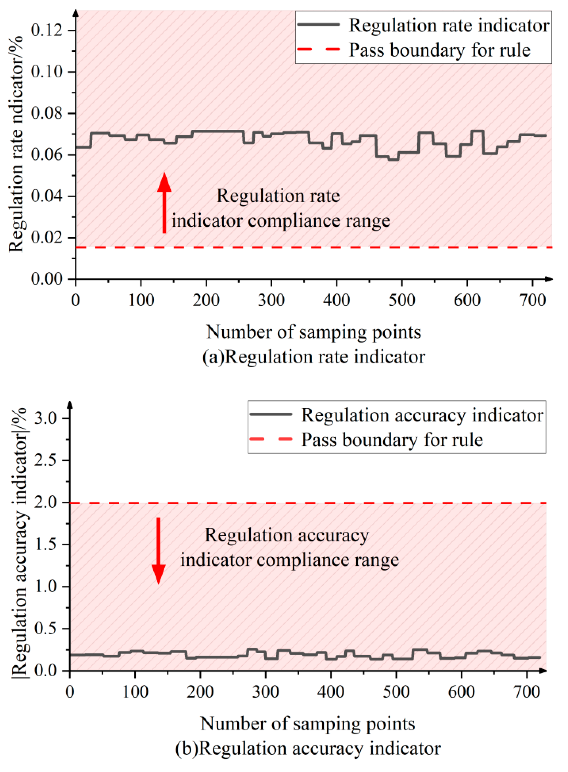
2.2.2. Regulation Rate Assessment

This is assessed based on the percentage shortfall between the monthly average regulation rate and the standard value. Specifically, for each 0.1% shortfall, 0.1 times the rated capacity in penalty points is imposed. The monthly average regulation rate is defined as the average of all regulation rates in a month, where the regulation rate of a single FR command is

$$K_1={\displaystyle \frac{\left|P_2-P_1-2\Delta \right|}{T_2-T_1}},$$

(1)

2.2.3. Regulation Accuracy Assessment

It is still assessed based on the monthly percentage shortfall, and the penalty points are calculated as 0.1 times the rated capacity for each 0.1% shortfall. The monthly average regulation accuracy is defined as the average of all regulation accuracies during the month, where the regulation accuracy of a single FR command is

$$K_2={\displaystyle \frac{{\displaystyle {\int }_{T_2}^{T_3}\left|P_2-P_g(t)\right|}dt}{T_3-T_2}},$$

(2)

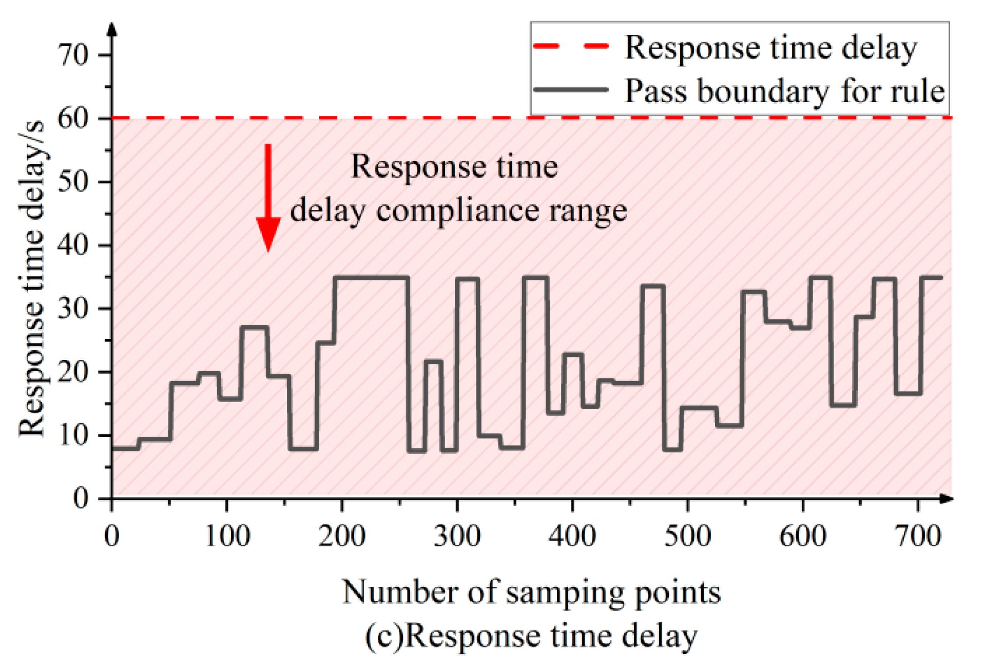
2.2.4. Compliance Rate Assessment of Response Time

This is assessed based on the monthly compliance rate of the response time, which is usually no less than 98%. Specifically, for each 1% shortfall, the penalty points are imposed at 0.1 times the rated capacity. The response time is defined as the time from the issuance of the FR command to the moment when the power output exceeds the dead-band, which is represented as

$$K_3=T_1-T_0,$$

(3)

The above FR performance sub-indicators determine the FR benefits of CHP plants.

3. Two-Stage Optimization Model for the CHP Plant

With the improvement in the operational flexibility of CHP units, the types of units in a plant have become more diverse, such as traditional extraction condensing units, back-pressure units, and extraction condensing units, cutting off the low-pressure cylinder [20]. Considering the cooperation between different types of CHP units and energy storage, optimization adopts plant-level dispatching to respond to FR commands instead of unit-level dispatching. A two-stage optimization model of the CHP plant with energy storage for FR sub-indicators’ performance is proposed. The first-stage model aims to maximize the benefits for the plant when responding to FR commands, which determines the values of FR performance sub-indicators and the curve of the power output of the CHP plant. The second-stage model focuses on optimal load dispatching of FR resources in the plant by the power output curve with the objective of minimizing the operating cost.

3.1. The First-Stage Optimization Model

3.1.1. Stage 1 Objective Function

The objective function is established by considering the electricity quantity compensation and penalties for failing to meet the FR performance sub-indicators’ standards. The function is

$$\max \left(R_{\mathrm{e}}-C_1-C_2-C_3\right),$$

(4)

where R_e represents regulation electricity quantity compensation of the CHP plant; and C₁, C₂, and C₃ represent the penalties about the regulation rate (K₁), regulation accuracy (K₂), and response time delay (K₃), respectively.

Taking a scheduling cycle as an example, it is assumed that the CHP power plant continuously responds to N FR commands during the scheduling cycle.

• Compensation model of regulation electricity quantity;

This model is computed by accumulating the amount of adjusted power, where the adjusted power must be in the same direction as the FR commands.

$$R_{\mathrm{e}}={\gamma }_0\times \left\{{\displaystyle \sum _{i=1}^N{\displaystyle \sum _{m=1}^M\max \left[\Delta W_{\mathrm{plant},i}\left(m\right),0\right]}}\right\},$$

(5)

$$\Delta W_{\mathrm{plant},i}(m)=\left\{\begin{array}{l}{\displaystyle {\int }_{(m-1)\Delta t}^{m\Delta t}\left(P_{\mathrm{plant},i}^{\mathrm{e}}(t)-\overline{P_{i-1}}\right)}dt , \overline{P_i}>\overline{P_{i-1}}\\ {\displaystyle {\int }_{(m-1)\Delta t}^{m\Delta t}\left(\overline{P_{i-1}}-P_{\mathrm{plant},i}^{\mathrm{e}}(t)\right)}dt , \overline{P_i}<\overline{P_{i-1}}\end{array}\right.,$$

(6)

where ${\gamma }_0$ represents the compensation factor; $N$ represents the number of FR commands; $M$ represents the number of sampling periods within the i-th FR command, which is calculated as $M={\displaystyle \frac{T_{3,i}-T_{0,i}}{\Delta t}}$, where $\Delta t$ represents the sampling interval time; $T_{0,i}$ and $T_{3,i}$ represent the start and end times of the i-th FR command, respectively; $\Delta W_{\mathrm{plant},i}(m)$ represents the regulation electricity quantity of the CHP plant during the m-th sampling period in response to the i-th FR command; $P_{\mathrm{plant},i}^{\mathrm{e}}(t)$ represents the electrical power output of the CHP plant at time t in response to the i-th FR command; and $\overline{P_i}$ and $\overline{P_{i-1}}$ represent the target power for the i-th and the preceding FR commands, respectively.

• Penalty models about sub-indicators;

As mentioned above, both the regulation rate and the regulation accuracy are assessed using statistical averages, as follows:

$$C_1={\gamma }_1\times \max \left\{0,\left[{\overline{K_1}}^{*}-\left(\raisebox{1ex}{${\displaystyle \sum _{i=1}^N\frac{K_{1,i}}{P_{\mathrm{N}}}}$}\!\left/ \!\raisebox{-1ex}{$N$}\right.\right)\right]\right\},$$

(7)

$$C_2={\gamma }_2\times \max \left\{0,\left[\left(\raisebox{1ex}{${\displaystyle \sum _{i=1}^N\frac{K_{2,i}}{P_{\mathrm{N}}}}$}\!\left/ \!\raisebox{-1ex}{$N$}\right.\right)-{\overline{K_2}}^{*}\right]\right\},$$

(8)

where ${\gamma }_1$ and ${\gamma }_2$ represent the penalty factors about the regulation rate and regulation accuracy, respectively; ${\overline{K_1}}^{*}$ and ${\overline{K_2}}^{*}$ represent the standards of the regulation rate and regulation accuracy for FR performance assessment, respectively; $K_{1,i}$ and $K_{2,i}$ are the regulation rate and regulation accuracy indicator responding to the i-th FR command, respectively; and P_N represents the rated capacity of the CHP plant.

The response time is assessed based on the compliance rate, as follows:

$$C_3={\gamma }_3\times \max \left[0,k-{\displaystyle \frac{{\displaystyle {\sum }_{i=1}^{N}g\left(K_{3,i}\right)}}{N}}\right],$$

(9)

$$g\left(K_{3,i}\right)=\left\{\begin{array}{l}1,K_{3,i}\le {\overline{K_3}}^{\ast }\\ 0,K_{3,i}>{\overline{K_3}}^{\ast }\end{array}\right.,$$

(10)

where ${\gamma }_3$ represents the penalty factor about the response time; ${\overline{K_3}}^{*}$ is the standard of the response time for FR performance assessment; $K_{3,i}$ is the response time when the CHP plant responds to the i-th FR command; and k represents the compliance rate, usually 98%, as mentioned above.

3.1.2. Stage 1 Constraints

The constraints of the first-stage model consider the impact of FR resource operations on sub-indicators, as well as the power–heat coupling of a CHP plant.

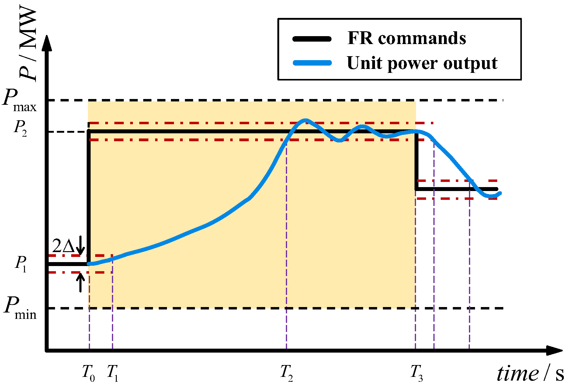
• Constraints of the FR performance sub-indicators

$${\displaystyle \frac{\left|\overline{P_i}-\overline{P_{i-1}}-2\Delta \right|}{T_{3,i}-T_{0,i}}}\le K_{1,i}\le \Delta P_{\mathrm{BESS}}^{\max }+\Delta P_d^{\max },$$

(11)

$$0\le K_{2,i}\le (\Delta P_{\mathrm{BESS}}^{\max }+\Delta P_d^{\max })\times (T_{3,i}-T_{2,i}),$$

(12)

$${\displaystyle \frac{\Delta }{\Delta P_{\mathrm{BESS}}^{\max }+\Delta P_d^{\max }}}\le K_{3,i}\le T_{3,i}-T_{0,i},$$

(13)

$$P_i(\zeta )\le \left\{\begin{array}{l}\overline{P_i}-\Delta +(\Delta P_{\mathrm{BESS}}^{\max }+\Delta P_d^{\max })\times (T_{3,i}-T_{2,i}) , \overline{P_i}>\overline{P_{i-1}}\\ \overline{P_i}+\Delta +(\Delta P_{\mathrm{BESS}}^{\max }+\Delta P_d^{\max })\times (T_{3,i}-T_{2,i}) , \overline{P_i}<\overline{P_{i-1}}\end{array}\right.,$$

(14)

$$P_i(\zeta )\ge \left\{\begin{array}{l}\overline{P_i}-\Delta -(\Delta P_{\mathrm{BESS}}^{\max }+\Delta P_d^{\max })\times (T_{3,i}-T_{2,i}) , \overline{P_i}>\overline{P_{i-1}}\\ \overline{P_i}+\Delta -(\Delta P_{\mathrm{BESS}}^{\max }+\Delta P_d^{\max })\times (T_{3,i}-T_{2,i}) , \overline{P_i}<\overline{P_{i-1}}\end{array}\right.,$$

(15)

$$\Delta P_d^{\max }={\displaystyle \sum _{d=1}^D{P}_{d,i}^{\max }},$$

(16)

where $P_{d,i}^{\max }$ represents the ramping rate of the d-th CHP unit for the i-th FR command, measured in MW/s; $\Delta P_{\mathrm{BESS}}^{\max }$ represents the power change rate of energy storage [21], measured in MW/s; $T_{2,i}$ represents the time when the power enters the dead-band of the i-th FR command, specifically, $T_{2,i}=T_{0,i}+K_{3,i}+{\displaystyle \frac{\left|\overline{P_i}-\overline{P_{i-1}}-2\Delta \right|}{K_{1,i}}}$; and $P_i(\zeta )$ represents the steady-state power after time $T_{2,i}$ during the i-th FR proceeding.

Moreover, the sub-indicators have the following time-coupling relationship when the CHP plant responds to the i-th FR command (Figure 1):

$$T_{3,i}-T_{0,i}={\displaystyle \frac{\left(\overline{P_i}-\overline{P_{i-1}}-2\Delta \right)}{K_{1,i}}}+{\displaystyle \frac{\left|\overline{P_i}-P_i(\zeta )\right|\times (T_{3,i}-T_{2,i})}{K_{2,i}}}+K_{3,i}.$$

(17)

• Power constraints for the CHP plant

$$\left|P_{\mathrm{plant},i}^{\mathrm{e}}(t)-P_{\mathrm{plant},i}^{\mathrm{e}}(t-1)\right|\le \Delta P_{BESS}^{\max }+{\displaystyle \sum _{d=1}^D\Delta P_{d,i}^{\max }}.$$

(18)

$$\left|P_{\mathrm{plant},i}^{\mathrm{e}}(t)-\overline{P_{i-1}}\right|<\Delta \hspace{1em}(T_{0,i}\le t<K_{3,i}).$$

(19)

$$\Delta \le \left|P_{\mathrm{plant},i}^{\mathrm{e}}(t)-\overline{P_{i-1}}\right|<\left|\overline{P_i}-\overline{P_{i-1}}\right|-\Delta \hspace{1em}(K_{3,i}\le t<T_{2,i}).$$

(20)

$$\left|P_{\mathrm{plant},i}^{\mathrm{e}}(t)-\overline{P_i}\right|\le \Delta \hspace{1em}(T_{2,i}\le t<T_{3,i}).$$

(21)

$$P_{\mathrm{plant},i}^{\mathrm{e}}(t)=\overline{P_i}\hspace{1em}(t=T_{3,i}).$$

(22)

$$P_{\mathrm{e}}^{\min }(P_{\mathrm{h}})\le P_{\mathrm{plant},i}^{\mathrm{e}}(t)\le P_{\mathrm{e}}^{\max }(P_{\mathrm{h}}).$$

(23)

where $P_{\mathrm{plant},i}^{\mathrm{e}}(t)$ represents the electrical power output of the CHP plant at time t under the i-th FR command; and $P_{\mathrm{e}}^{\max }(P_{\mathrm{h}})$ and $P_{\mathrm{e}}^{\min }(P_{\mathrm{h}})$ represent the maximum and minimum electrical power outputs of the CHP plant when the heat power is $P_{\mathrm{h}}$.

The decision variable of first-stage optimization model is

$$\left\{K_{1,i},K_{2,i},K_{3,i},P_{\mathrm{plant},i}^{\mathrm{e}}(t)\right\},i\in N.$$

(24)

3.2. The Second-Stage Optimization Model

3.2.1. Stage 2 Objective Function

After obtaining the electrical power output of the CHP plant from the first-stage optimization model, the objective function of the second-stage optimization model is to minimize the operating cost of the CHP plant with energy storage.

$$\min {\displaystyle \sum _{t=T_{0,i}}^{T_{3,i}}\left({\displaystyle \sum _{p=1}^{n_1}{F}_{\mathrm{Ex},p,t}+{\displaystyle \sum _{j=1}^{n_2}{F}_{\mathrm{BP},j,t}}}\right)\cdot \tau +F_{\mathrm{bat},i}}.$$

(25)

where $\tau$ represents the time interval; $F_{\mathrm{bat},i}$ represents the operating cost of energy storage; n₁ and n₂ represent the numbers of extraction condensing CHP units (including the units cutting off the low-pressure cylinder) and back-pressure CHP units; and, correspondingly, $F_{\mathrm{Ex},p,t}$ and $F_{\mathrm{BP},j,t}$ represent the coal consumption costs of the two types of CHP units at time t, calculated as follows:

• Coal consumption cost [22];

$$\left\{\begin{array}{l}{F}_{\mathrm{Ex},p,t}=a_{\mathrm{Ex},p}{P}_{\mathrm{con},p,t}^2+b_{\mathrm{Ex},p}{P}_{\mathrm{con},p,t}+c_{\mathrm{Ex},p}\\ P_{\mathrm{con},p,t}=P_{\mathrm{Ex},p,t}^{\mathrm{e}}+c_{\mathrm{v},p}{P}_{\mathrm{Ex},p,t}^{\mathrm{h}}\end{array}\right..$$

(26)

where $P_{\mathrm{Ex},p,t}^{\mathrm{e}}$ and $P_{\mathrm{Ex},p,t}^{\mathrm{h}}$ represent the power and heat output of the p-th extraction condensing CHP unit at time t; $a_{\mathrm{Ex},p}$, $b_{\mathrm{Ex},p}$, and $c_{\mathrm{Ex},p}$ represent the coal consumption characteristic coefficients of the p-th unit, measured in t/MW²h, t/MWh, and t/h, respectively; and $c_{v,p}$ represents the heat to electric power impact factor of the extraction condensing CHP unit.

$$\left\{\begin{array}{l}{F}_{\mathrm{BP},j,t}=a_{\mathrm{BP},j}{P}_{\mathrm{con},j,t}^2+b_{\mathrm{BP},j}{P}_{\mathrm{con},j,t}+c_{\mathrm{BP},j}\\ P_{\mathrm{con},j,t}={\displaystyle \frac{c_{\mathrm{m}1,j}(P_{\mathrm{BP},j,t}^{\mathrm{e}}+P_{\mathrm{BP},j,t}^{\mathrm{h}})}{1+c_{\mathrm{m}1,j}}}\end{array}\right..$$

(27)

where $P_{\mathrm{BP},j,t}^{\mathrm{e}}$ and $P_{\mathrm{BP},j,t}^{\mathrm{h}}$ represent the heat and power output of the j-th back-pressure CHP unit at time t; $a_{\mathrm{BP},j}$, $b_{\mathrm{BP},j}$, and $c_{\mathrm{BP},j}$ represent the coal consumption characteristic coefficients of the j-th unit, measured in t/MW²h, t/MWh, and t/h, respectively; and $c_{\mathrm{m}1,j}$ represents the heat to electric power impact factor of the back-pressure CHP unit.

• Operating cost of the energy storage;

The operating cost of energy storage includes the maintenance cost (F_op) and the allocation of investment cost (F_PV), both of which are related to the rated capacity of energy storage. These costs are considered as fixed and allocated over the operating period. On an annual basis, the operating cost is

$$F_{\mathrm{APV}}=F_{\mathrm{op}}+F_{\mathrm{PV}}\times {\displaystyle \frac{r{(1+r)}^{T_{\mathrm{float}}}}{{(1+r)}^{T_{\mathrm{float}}}-1}}.$$

(28)

where r represents the discount rate; and T_float represents the theoretical floating life of energy storage. When calculating the operating cost within an FR command period, there is

$$F_{\mathrm{bat},i}={\displaystyle \frac{\left(T_{3,i}-T_{0,i}\right)}{24}}\times {\displaystyle \frac{F_{\mathrm{APV}}}{365}}.$$

(29)

3.2.2. Stage 2 Constraints

• Power and heat load constraints;

$$\left\{\begin{array}{l}{P}_{\mathrm{plant},i}^{\mathrm{e}}(t)={\displaystyle \sum _{p=1}^{n_1}\left(P_{\mathrm{Ex},p,t}^{\mathrm{e}}\right)+{\displaystyle \sum _{j=1}^{n_2}\left(P_{\mathrm{BP},j,t}^{\mathrm{e}}\right)+P_{\mathrm{BESS},t}^{\mathrm{e}}}}\\ P_{\mathrm{plant},i}^{\mathrm{h}}(t)={\displaystyle \sum _{p=1}^{n_1}\left(P_{\mathrm{Ex},p,t}^{\mathrm{h}}\right)+{\displaystyle \sum _{j=1}^{n_2}\left(P_{\mathrm{BP},j,t}^{\mathrm{h}}\right)}}\end{array}\right..$$

(30)

• The feasible operation region constraints of CHP units;

(1)

The extraction condensing CHP unit (including the units cutting off the low-pressure cylinder);

$$\left\{\begin{array}{l}{P}_{\mathrm{Ex},p,t}^{\mathrm{e}}\le I_{t,p}\left(P_{\mathrm{Con},p}^{\mathrm{e},\max }-c_{v,p}{P}_{\mathrm{Ex},p,t}^{\mathrm{h}}\right)\\ P_{\mathrm{Ex},p,t}^{\mathrm{e}}\ge I_{t,p}\left(P_{\mathrm{Con},p}^{\mathrm{e},\max }-c_{v,p}{P}_{\mathrm{Ex},p,t}^{\mathrm{h}}\right)\\ P_{\mathrm{Ex},p,t}^{\mathrm{h}}\le P_{\mathrm{Ex},p}^{\mathrm{h},\max }+I_{t,p}\cdot \Delta P_0^{\mathrm{h}}\\ P_{\mathrm{Ex},p,t}^{\mathrm{h}}\ge I_{t,p}\cdot ({\displaystyle \frac{P_{\mathrm{Con},p}^{\mathrm{e},\min }-P_0^{\mathrm{e}}}{c_{\mathrm{m},p}+c_{\mathrm{v},p}}}+\Delta P_0^{\mathrm{h}})\\ P_{\mathrm{Ex},p,t}^{\mathrm{e}}\ge I_{t,p}[P_0^{\mathrm{e}}+c_{\mathrm{m}}{P}_{\mathrm{Ex},p,t}^{\mathrm{h}}-(c_{\mathrm{m},p}+c_{\mathrm{v},p})\Delta P_0^{\mathrm{h}}]\\ P_{\mathrm{Ex},p,t}^{\mathrm{e}}\ge (1-I_{t,p})\cdot \max \{P_{\mathrm{Con},p}^{\mathrm{e},\min }-c_{\mathrm{v},p}{P}_{\mathrm{Ex},p,t}^{\mathrm{h}}, P_0^{\mathrm{e}}+c_{\mathrm{m},p}{P}_{\mathrm{Ex},p,t}^{\mathrm{h}}\}\end{array}\right..$$

(31)

where $P_0^{\mathrm{e}}$ represents the intercept of the unit’s operating curve on the vertical axis; c_m,p represents the maximum power-to-heat ratio under the extraction steam working condition; and $I_{t,p}$ is the Boolean variable determining the low-pressure cylinder cut-out status (1 = cut-out, 0 = not cut-out).

(2)

The back-pressure CHP unit;

$$\left\{\begin{array}{l}{P}_{\mathrm{BP},j,t}^e\le \min \{c_{\mathrm{m}1,j}{P}_{\mathrm{BP},j,t}^{\mathrm{h}},{\displaystyle \frac{c_{\mathrm{m}1,j}+1}{c_{\mathrm{m}1,j}}}{P}_{\mathrm{BP},j}^{\mathrm{e},\max }-P_{\mathrm{BP},j,t}^{\mathrm{h}}\}\\ P_{\mathrm{BP},j,t}^{\mathrm{e}}\ge \max \{c_{\mathrm{m}2,j}{P}_{\mathrm{BP},j,t}^{\mathrm{h}},{\displaystyle \frac{c_{\mathrm{m}1,j}+1}{c_{\mathrm{m}1,j}}}{P}_{\mathrm{BP},j}^{\mathrm{e},\min }-P_{\mathrm{BP},j,t}^{\mathrm{h}}\}\\ {\displaystyle \frac{P_{\mathrm{BP},j}^{\mathrm{e},\min }}{c_{\mathrm{m}1,j}}}\le P_{\mathrm{BP},j,t}^{\mathrm{h}}\le P_{\mathrm{BP},j}^{\mathrm{h},\max }\end{array}\right..$$

(32)

where $c_{\mathrm{m}1,j}$ and $c_{\mathrm{m}2,j}$ represent the heat to electric power impact factors under pure back-pressure and maximum extraction steam working conditions, respectively.

• The ramping rate constraints of CHP units;

(3)

The extraction condensing CHP unit;

$$\left\{\begin{array}{c}(P_{\mathrm{Ex},p,t}^{\mathrm{e}}+c_{\mathrm{v},p}{P}_{\mathrm{Ex},p,t}^{\mathrm{h}})-(P_{\mathrm{Ex},p,t-1}^{\mathrm{e}}+c_{\mathrm{v},p}{P}_{\mathrm{Ex},p,t-1}^{\mathrm{h}})\le P_{\mathrm{Ex},p}^{\mathrm{up}}\\ (P_{\mathrm{Ex},p,t-1}^{\mathrm{e}}+c_{\mathrm{v},p}{P}_{\mathrm{Ex},p,t-1}^{\mathrm{h}})-(P_{\mathrm{Ex},p,t}^{\mathrm{e}}+c_{\mathrm{v},p}{P}_{\mathrm{Ex},p,t}^{\mathrm{h}})\ge P_{\mathrm{Ex},p}^{\mathrm{dn}}\end{array}\right..$$

(33)

(4)

The back-pressure CHP unit;

$$\left\{\begin{array}{c}({\displaystyle \frac{c_{\mathrm{m}1,j}(P_{\mathrm{BP},j,t}^{\mathrm{e}}+P_{\mathrm{BP},j,t}^{\mathrm{h}})}{1+c_{\mathrm{m}1,j}}})-({\displaystyle \frac{c_{\mathrm{m}1,j}(P_{\mathrm{BP},j,t-1}^{\mathrm{e}}+P_{\mathrm{BP},j,t-1}^{\mathrm{h}})}{1+c_{\mathrm{m}1,j}}})\le P_{\mathrm{BP},j}^{\mathrm{up}}\\ ({\displaystyle \frac{c_{\mathrm{m}1,j}(P_{\mathrm{BP},j,t-1}^{\mathrm{e}}+P_{\mathrm{BP},j,t-1}^{\mathrm{h}})}{1+c_{\mathrm{m}1,j}}})-({\displaystyle \frac{c_{\mathrm{m}1,j}(P_{\mathrm{BP},j,t}^{\mathrm{e}}+P_{\mathrm{BP},j,t}^{\mathrm{h}})}{1+c_{\mathrm{m}1,j}}})\le P_{\mathrm{BP},j}^{\mathrm{dn}}\end{array}\right..$$

(34)

where $P_{\mathrm{Ex},p}^{\mathrm{up}}$, $P_{\mathrm{Ex},p}^{\mathrm{dn}}$, $P_{\mathrm{BP},p}^{\mathrm{up}}$, and $P_{\mathrm{BP},p}^{\mathrm{dn}}$ represent the upper and lower ramp rate limits for different types of CHP units, with the subscript Ex representing the extraction condensing CHP unit (including the units cutting off the low-pressure cylinder) and BP representing the back-pressure CHP unit.

• SOC constraints of energy storage;

To ensure the longevity of the energy storage and prevent operation at too high or low an SOC level, the upper and lower SOC limits should be set to 0.9 and 0.1, respectively.

$$SO{C}_{t+1}=SO{C}_t+{\displaystyle \frac{P_{\mathrm{BESS},\mathrm{ch},t}\cdot {\eta }_{\mathrm{ch}}\cdot △t}{C_{\mathrm{BESS}}}}-{\displaystyle \frac{P_{\mathrm{BESS},\mathrm{dis},t}\cdot △t}{{\eta }_{\mathrm{dis}}\cdot C_{\mathrm{BESS}}}}.$$

(35)

$$\left\{\begin{array}{c}0.1\le SO{C}_t\le 0.9\\ 0\le P_{\mathrm{BESS},\mathrm{ch},t}\le P_{\mathrm{BESS}}\\ 0\le P_{\mathrm{BESS},\mathrm{dis},t}\le P_{\mathrm{BESS}}\\ y_{\mathrm{Ess},\mathrm{ch},t}+y_{\mathrm{Ess},\mathrm{dis},t}\le 1\end{array}\right..$$

(36)

where $SO{C}_t$ represents the SOC of energy storage at time t; $P_{\mathrm{BESS}}$ represents the rated charging or discharging power; $C_{\mathrm{BESS}}$ represents the rate capacity; $P_{\mathrm{BESS},\mathrm{ch},t}$ and $P_{\mathrm{BESS},\mathrm{dis},t}$ represent the charging and discharging powers at time t, respectively; ${\eta }_{\mathrm{ch}}$ and ${\eta }_{\mathrm{dis}}$ represent the charging and discharging efficiencies, respectively; and $y_{\mathrm{ESS},\mathrm{ch},t}$ and $y_{\mathrm{ESS},\mathrm{dis},t}$ represent Boolean variables indicating charging and discharging statuses.

• Operating cost constraints of energy storage

To ensure that the cycle life of energy storage is no shorter than its floating life, the number of equivalent full cycles ($n_{\mathrm{eq}}^{100\%}$) should be limited for every FR command:

$$n_{\mathrm{eq}}^{100\%}\le N_{\lim }^{\mathrm{day}}\cdot {\displaystyle \frac{\left(T_{3,i}-T_{0,i}\right)}{24}}.$$

(37)

where $N_{\lim }^{\mathrm{day}}$ represents the maximum number of daily equivalent cycles corresponding to floating life; and $n_{\mathrm{eq}}^{100\%}$ is related to the maximum depth of discharge (DOD) and relative DOD, which can be derived using the nonlinear models in Refs. [23,24].

The decision variables of the second-stage optimization model are

$$\left\{P_{\mathrm{Ex},p,t}^{\mathrm{e}},P_{\mathrm{Ex},p,t}^{\mathrm{h}}{P}_{\mathrm{BP},j,t}^{\mathrm{e}},P_{\mathrm{BP},j,t}^{\mathrm{h}},P_{\mathrm{BESS},\mathrm{ch},t},P_{\mathrm{BESS},\mathrm{dis},t}\right\}.$$

(38)

3.3. Prediction Model of FR Commands

The key to achieving the output of CHP units with energy storage lies in accurately predicting the FR commands based on the time coupling of energy storage. In order to dynamically correct the prediction result, the deviation between the actual FR commands and the predicted value is used as an input feature based on the Long Short-Term Memory (LSTM) neural network prediction model.

3.3.1. Historical Data Pre-Process

Historical data are an important part of the time-series forecasting problem. The historical time series of FR commands is pre-processed using the STL method [25], as follows:

$$P_{\mathrm{AGC}}=P_{\mathrm{AGC},\mathrm{S}}+P_{\mathrm{AGC},\mathrm{T}}+P_{\mathrm{AGC},\mathrm{I}}.$$

(39)

where P_AGC represents the historical time series of FR commands; and P_AGC,S, P_AGC,T, and P_AGC,I represent the seasonal fluctuation, long-term trend, and irregular fluctuation components, respectively.

3.3.2. Single-Step Prediction Model for FR Commands

The seasonal fluctuation component is regular and can be extrapolated from the historical time series. The long-term trend and irregular fluctuation components need to be achieved by the LSTM neural network model training with the historical time series of FR commands. Then, the short-term prediction of the FR commands for the next scheduling period is obtained by adding the prediction results of the three components as follows:

$$\left\{\begin{array}{l}{P}_{\mathrm{AGC},n+1}=P_{\mathrm{AGC},\mathrm{S},n+1}+P_{\mathrm{AGC},\mathrm{T},n+1}+P_{\mathrm{AGC},\mathrm{I},n+1}\\ P_{\mathrm{AGC},\mathrm{T},n+1}=f_1(P_{\mathrm{AGC},\mathrm{T},n},\dots ,P_{\mathrm{AGC},\mathrm{T},n-d})\\ P_{\mathrm{AGC},\mathrm{I},n+1}=f_2(P_{\mathrm{AGC},\mathrm{I},n},\dots ,P_{\mathrm{AGC},\mathrm{I},n-d})\end{array}\right..$$

(40)

where $P_{\mathrm{AGC},n+1}$ represents the short-term prediction result of the FR commands for period n + 1; $P_{\mathrm{AGC},\mathrm{S},n+1}$, $P_{\mathrm{AGC},\mathrm{T},n+1}$, and $P_{\mathrm{AGC},\mathrm{I},n+1}$ represent the seasonal fluctuation, the long term trend, and irregular fluctuation components for period n + 1, respectively; and $f_1$ and $f_2$ represent the single-step prediction models for the long-term trend and irregular fluctuation components, which are trained from corresponding data for historical periods from (n − d) to n.

3.3.3. Multi-Step Prediction Model for FR Commands

A recursive strategy is used for multi-step prediction. The deviation between actual and predicted values of the latest period of FR commands is used as an additional input to dynamically correct the multi-step prediction model, as follows:

$$P_{\mathrm{AGC},n+h}=g\left(P_{\mathrm{AGC},n+h-1},P_{\mathrm{AGC},n+h-2},\dots ,P_{\mathrm{AGC},n+h-d},\Delta P_{\mathrm{AGC},n}\right).$$

where $P_{\mathrm{AGC},n+h}$ represents the prediction result of FR commands in period (n + h), while g represents the multi-step prediction model; h (h ≥ 2) represents the length of the forward-predicted period; and $\Delta P_{\mathrm{AGC},n}$ represents the deviation between the actual and predicted FR commands at period n.

In order to quantitatively compare the prediction accuracy of the FR command prediction model in Section 3.3, the prediction models in Refs. [26,27] are evaluated using mean absolute error (MAE) and coefficient of determination (R²), respectively. The comparison results are detailed in Appendix A.1.

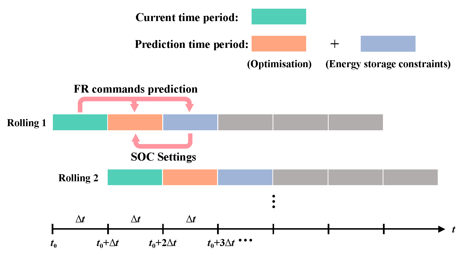
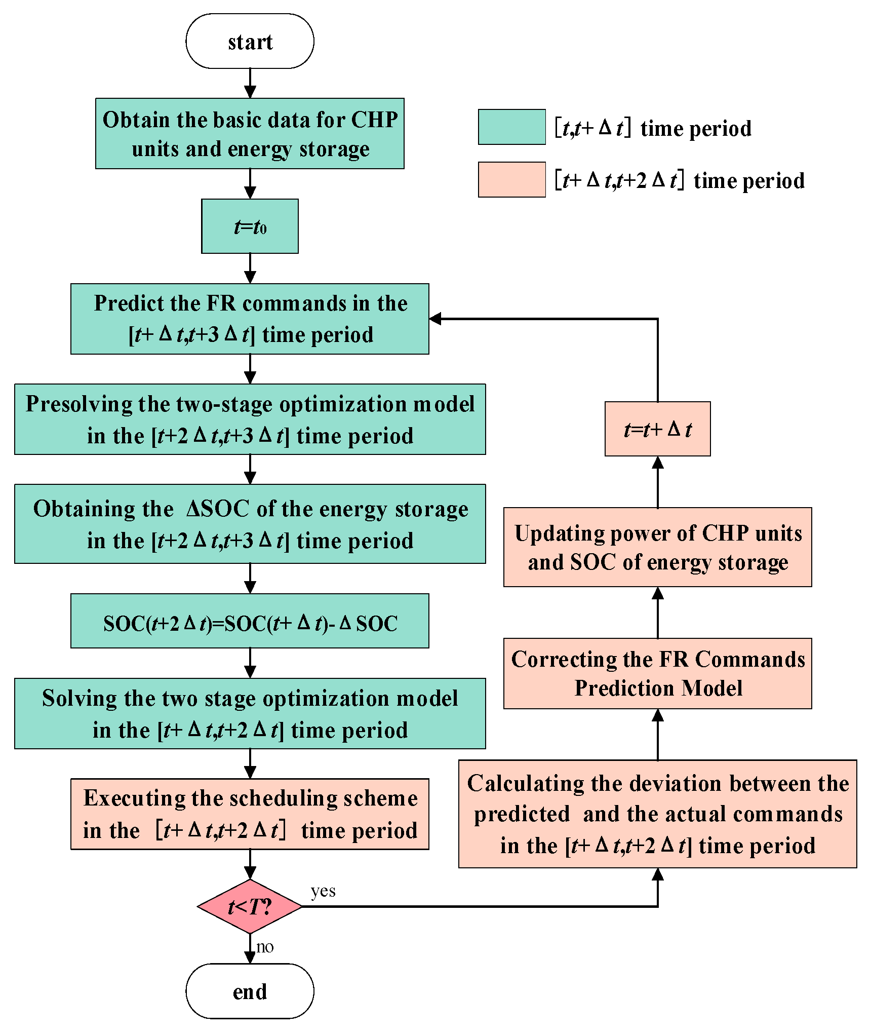
3.4. The Two-Stage Real-Time Rolling Optimization FR Strategy

Based on the prediction of the real-time FR commands, the MPC method is used for rolling optimization, which can improve energy storage utilization and enhance the ability of a CHP plant to follow FR commands in real time. The FR system architecture for CHP units with energy storage is detailed in Appendix A.2. The time-rolling process operates as shown in Figure 2.

Step 1 (initialization update): At the time t₀, using the latest load distribution, the states of the CHP units and energy storage are initialized for the FR period [t₀, t₀ + Δt], including the power/heat output, and SOC.

Step 2 (FR command prediction): The FR commands for the next two scheduling periods [t₀ + Δt, t₀ + 3Δt] are predicted based on the prediction model in Section 3.3.

Step 3 (setting the initial SOC): In order to ensure that energy storage can fully respond to FR in the period [t₀ + 2Δt, t₀ + 3Δt], the SOC change in energy storage (ΔSOC) can be precomputed and optimized according to the prediction FR commands in the period [t₀ + 2Δt, t₀ + 3Δt]; then, the SOC at time t₀ + 2Δt is set as SOC(t₀ + Δt) − ΔSOC so the energy storage has enough capacity.

Step 4 (two-stage optimization and execution for FR): By solving the two-stage model based on the predicted FR commands in the period [t₀ + Δt, t₀ + 2Δt], the optimal load distribution is obtained and executed to respond to the FR commands in this period.

Step 5 (FR command correction and rolling optimization): The above steps are repeated in the next period [t₀ + Δt, t₀ + 2Δt] (note: the deviation between the actual and predicted FR commands in the current period is used as one of the inputs in Step 2 to dynamically correct the FR command prediction model).

The flowchart of the two-stage real-time rolling optimization FR strategy of the CHP units with energy storage is shown in Figure 3.

4. Analysis of Case Studies

4.1. Basic Data

In this section, the CHP plant in Northeast China is studied. There are four 350 MW CHP units, where Unit #1 is a back-pressure unit, Unit #2 has the ability to flexibly cut off the low-pressure cylinder, and Units #3 and #4 are extraction condensing units. The characteristics of the four units are shown in Ref. [28]. The heat load is 892 MW, which is approximately 52% of the maximum heating capacity of the CHP plant, and it changes insignificantly in short periods. The standard, penalty, and compensation factors under the rule of FR performance assessment for the CHP units in the plant are shown in

Table 1. The FR indicators’ standard, penalty, and compensation factors.

The Standard, Penalty, and Compensation Factors	Values
Lower limit of regulation rate/s−1	0.017
Upper limit of regulation accuracy/%	±2
Upper limit of response time delay/s	60
Lower limit of pass compliance rate boundary/%	98
Regulation electricity quantity compensation factor/$·MWh−1	16.59
Penalty factor for regulation rate/$·point−1	1382.74
Penalty factor for regulation accuracy/$·point−1	1382.74
Penalty factor for compliance rate/$·point−1	138.27
Input steps in the single-step prediction model	8

. The rated power/capacity of energy storage is 42 MW/21 MWh; the construction cost of the energy storage is USD 414.82 (CNY 3000)/kWh without considering magnification characteristics [22]; the initial SOC of energy storage is 0.5; and the charging/discharging efficiency is 0.95.

4.2. Comparison with Existing Strategies

The two-stage real-time rolling FR strategy is compared with two commonly used strategies—the full power compensation strategy and the decomposition strategy of FR commands [28]—in terms of effectiveness and economy.

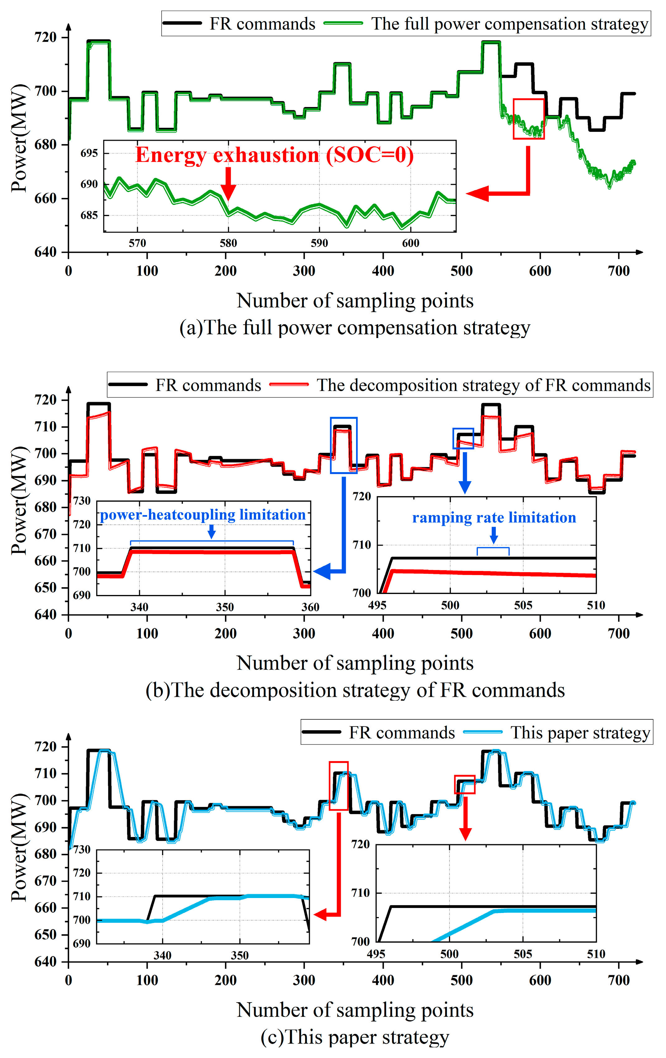
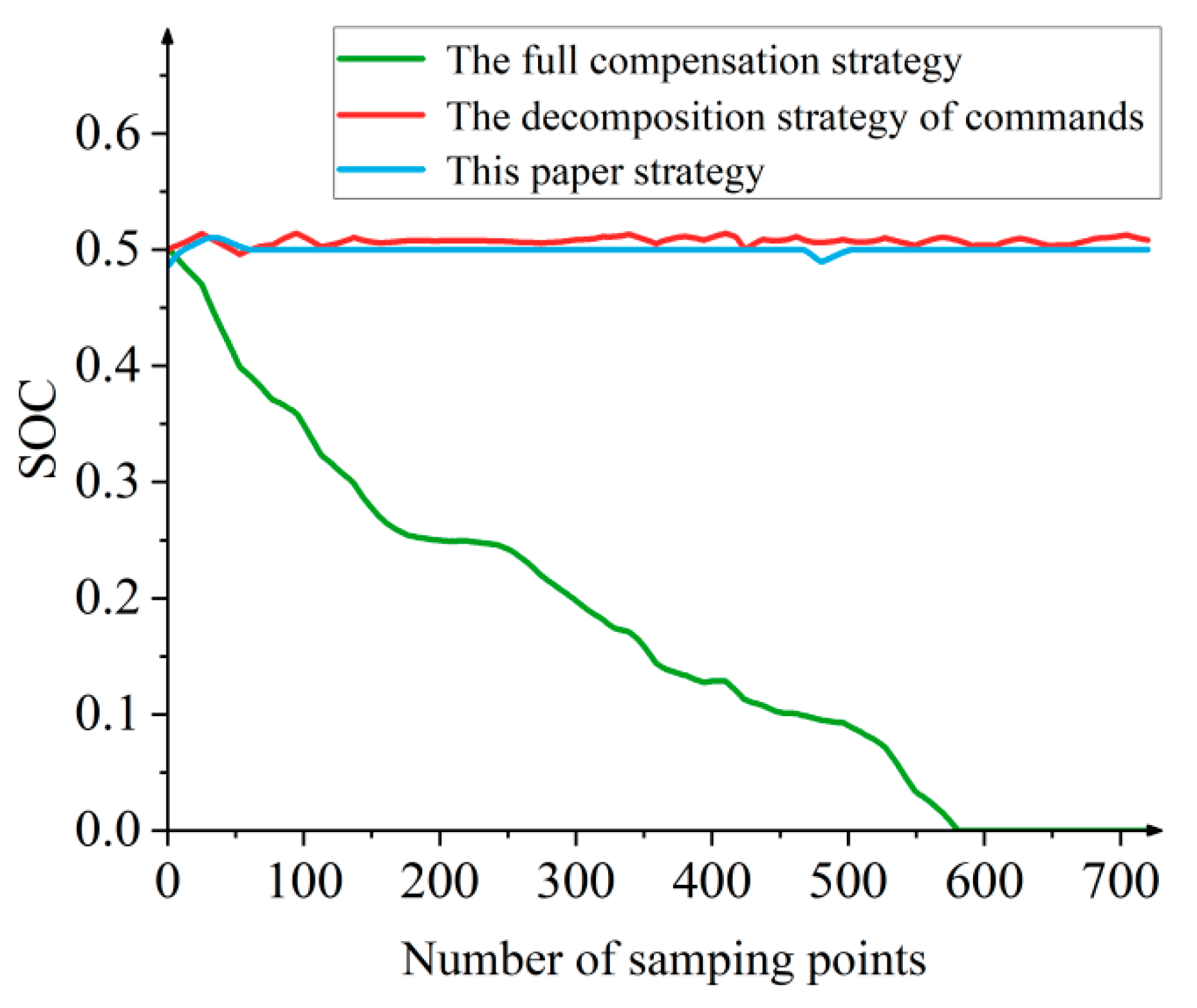
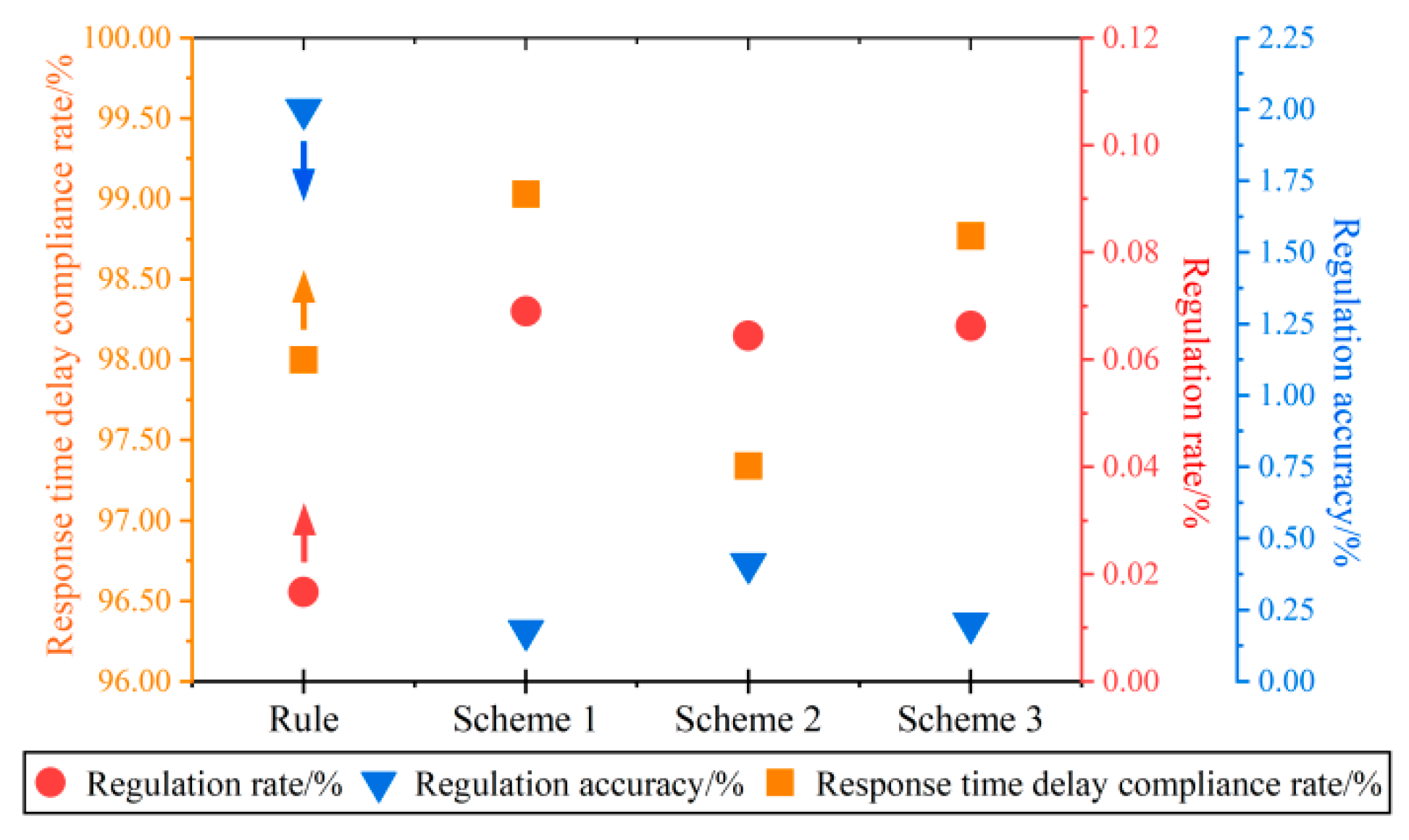
4.2.1. Comparison of Response Effects

The sub-indicators and regulation electricity quantities’ compensation are shown in Figure 4. The response of the plant under the three FR strategies in 60 min (12 scheduling periods, with a sampling interval is 5 s) is shown in Figure 5.

The full power compensation strategy is simple and rapid, but energy storage fails to compensate due to energy exhaustion, for example, periods 549–610 in Figure 5a. This leads to insufficient response to FR commands.

The decomposition strategy using the EEMD method can decompose the FR commands into low- and high-frequency components, but it does not utilize the power complementarity between CHP units and energy storage. As shown in Figure 5b, the rate of change in low-frequency commands for CHP units exceeds the ramping rate limitation (e.g., in periods 502–504). Meanwhile, the maximum power output (708.46 MW) is limited due to power and heat coupling. This renders the plant unable to meet the requirements of the low-frequency FR commands (e.g., in periods 341–358), worsening the regulation accuracy. These demands may all be compensated for by energy storage.

The FR performance sub-indicators responding to the FR commands are shown in Appendix A.3. The regulation rate (0.067%), regulation accuracy (0.19%), and response time delay compliance rate (98.97%) all meet the standards in Northeast China. The regulation electricity quantity compensation is USD 78.64 (CNY 568.69) with no penalty. Based on the above sub-indicators, the overall power output of the CHP plant is obtained as shown with the blue curve in Figure 5c. Furthermore, the load distribution result of second-stage optimization takes into account the capacity support capability of CHP units, the fast regulation capability of energy storage, and the complementation between CHP units and energy storage. Then, the problems of an insufficient ramping rate of CHP units (above-mentioned period 502–504) and electric power output due to heat constrains (mentioned period 341–358) disappear.

4.2.2. Comparison of FR Operating Cost and Benefits

According to Section 3.2, the details of FR operating costs and regulation electricity quantity compensations for the three FR strategies are shown in

Table 2. Comparison of operating cost and compensation.

Strategies	Full Power	Decomposition	This Paper
Energy storage cost/$	1102.35	412.17	247.58
CHP unit cost/$	13,071.92	13,074.69	13,073.31
FR operating cost/$	14,174.27	13,486.86	13,320.89
Electricity quantities’ compensation/$	53.94	70.54	81.60

. The two-stage strategy proposed in this paper demonstrates a superior performance compared to the other strategies in terms of both operating cost and compensation.

• Analysis of FR operating cost;

According to Table 2, the obvious reduction in cost is the cost of energy storage. This is due to the avoidance of charging at high power (e.g., the period 258–294) and discharging at a low SOC (e.g., the period 93–111) by the two-stage strategy. The SOC of energy storage by different strategies is shown in Figure 6.

Under the full power compensation strategy with the initial SOC setting as 0.5, the SOC of the energy storage continually decreases, meaning FR performance distinctly relies on the initial SOC value. Consequently, the longer the energy storage discharges at a low SOC (e.g., period 549–610), the higher the operating cost.

Meanwhile, the decomposition strategy leads to frequent and obvious regulation of energy storage, which increases the operating cost significantly. For example, the storage is regulated at 10.42 MW during the period 111–113 and 11 times during the period 424–608.

The strategy proposed in this paper is driven by the second-stage objective function to ensure the lowest operating cost of CHP units and energy storage. It can be seen that the back-pressure CHP unit and the extraction condensing CHP unit cutting off the low-pressure cylinder are operated in a high-energy-efficiency state, the former operates near the maximum output in the pure back-pressure state, and the latter operates in the state of cutting off the low-pressure cylinder throughout the FR process (Figure 7). At the same time, the SOC stabilizes at about 0.5, ensuring continuous energy storage operation and effectively reducing its FR operating cost. With the above optimal distribution of CHP units and energy storage, the FR operating cost of this paper’s strategy is the lowest among the three strategies.

• Analysis of regulation electricity quantities’ compensation

As shown in Table 2, the strategy proposed in this paper is effectively driven by the first-stage objective function, which increases the regulation electricity quantity by 31.51% compared with the full compensation strategy and by 10.98% compared with the decomposition strategy of FR commands.

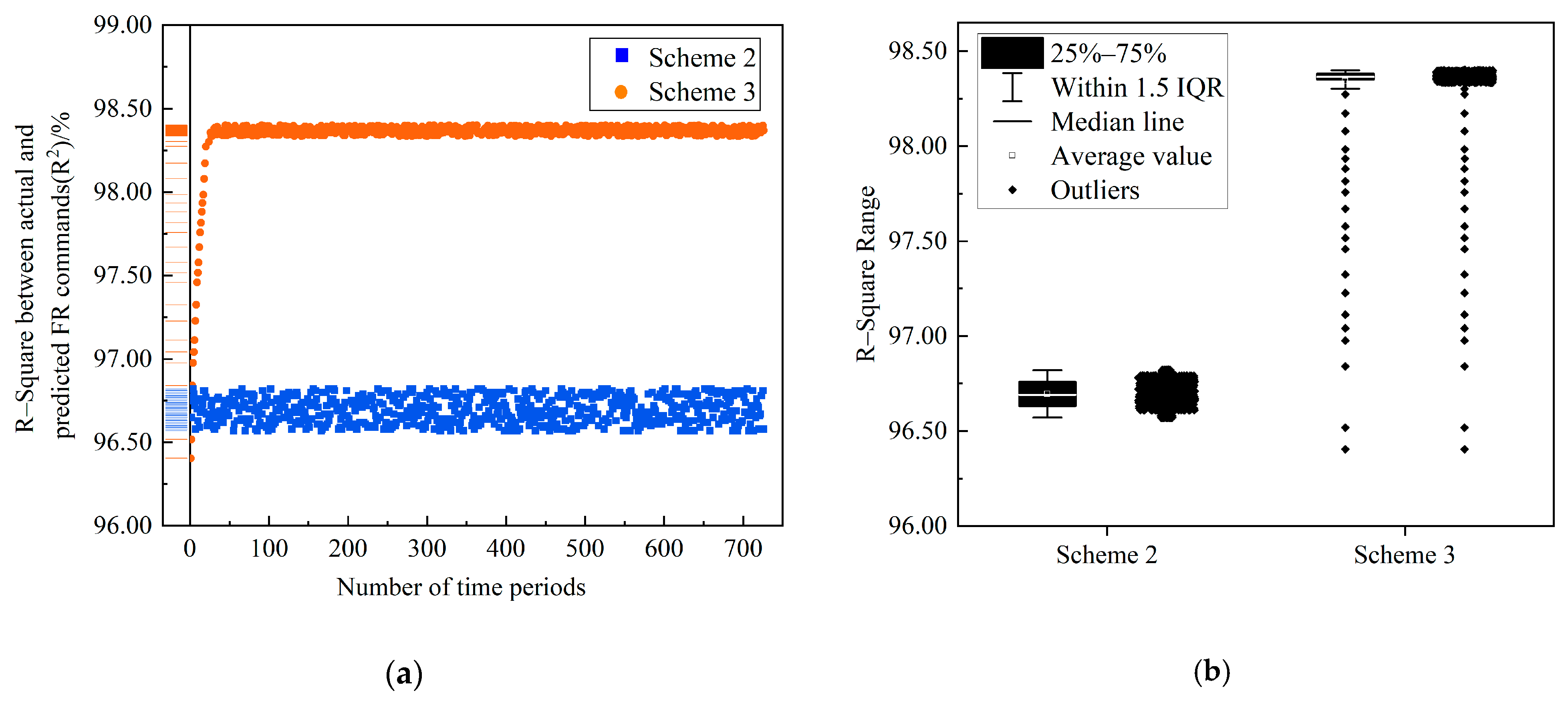
4.3. Analysis of the Impact of Rolling Optimization on FR Effects

The FR effects of the strategy in this paper are related to the errors of the FR command prediction model. To address time-accumulating prediction errors and maintain prediction accuracy, the FR command prediction model is dynamically corrected through the rolling optimization algorithm. To verify the impact of the dynamic correction step on FR performance, the following three schemes are set up to compare the response to FR commands in a month.

Scheme 1: Assuming no prediction errors;

Scheme 2: Obtaining FR commands by the traditional prediction method;

Scheme 3: Using the dynamic correction of this paper.

The FR performance sub-indicators of the CHP plant in response to FR commands under each scheme are shown in Figure 8.

The FR commands in scheme 1 are real (ideal case), so the response is optimal and serves as the control group for comparison with other schemes. The three FR performance sub-indicators of scheme 3 all meet the standards. This shows that the strategy of this paper is effective for real-time FR.

As shown in Figure 9, scheme 3 has a better response effect than scheme 2 because scheme 3 has fewer errors in the FR commands’ prediction through dynamic correction. The coefficient of determination (R²) measures how well the predicted FR commands match the actual values, where values closer to 1 indicate a better prediction accuracy. As shown in Figure 9, the predicted FR commands of scheme 3 are close to the actual values over time. This is the key reason why the time delay compliance rate and regulation accuracy are significantly improved, while the regulation rate improvement is not clear because of the CHP units.

5. Conclusions

For the assessment from FR performance sub-indicators in the Northeast Chinese market, this paper proposes a two-stage real-time rolling optimization FR strategy for CHP units with energy storage, verified by real operating data from a CHP plant in Northeast China. The conclusions are summarized below.

(1)

The two-stage optimization model in this paper takes the overall FR benefits and operating cost of a CHP plant as optimization objectives, respectively. Through the energy complementarity between CHP units and energy storage, the optimal distribution of plant-level electrical and heat power is achieved while considering the improvement of FR performance sub-indicators. In terms of FR benefits, this paper’s strategy improves by 31.51% and 10.98% compared with the full power compensation strategy and FR command decomposition strategy, respectively. In terms of FR operating costs, there are reductions of 6.41% and 1.25%, respectively.

(2)

The two-stage real-time rolling FR strategy in this paper is based on the FR command prediction model and uses the rolling optimization algorithm, which includes a dynamic correction link. By introducing the deviation between the actual and predicted commands into the rolling process, the prediction accuracy can reach 98.34% after about 23 rolls, which is 1.65% higher than the traditional method. This reduction in FR command prediction errors effectively enhances the regulation accuracy and the response delay compliance of the FR process.

The above strategy serves as an effective model for most CHP plants in Northeast China with which to respond to FR requirements. The impact of flexibility in resources, such as heat storage tanks or electric boilers, on the FR performance across CHP plants should be further explored.

References

1. Shair, J.; Li, H.Z.; Hu, J.B.; Xie, X.R. Power system stability issues, classifications and research prospects in the context of high-penetration of renewables and power electronics. Renew. Sustain. Energy Rev. 2021, 145, 111111. [Google Scholar]
2. Hatziargyriou, N.; Milanovic, J.; Rahmann, C.; Ajjarapu, V.; Canizares, C.; Erlich, I.; Hill, D.; Hiskens, I.; Kamwa, I.; Pal, B.; et al. Definition and classification of power system stability–revisited & extended. IEEE Trans. Power Syst. 2020, 36, 3271–3281. [Google Scholar]
3. Ameli, H.; Qadrdan, M.; Strbac, G. Coordinated operation strategies for natural gas and power systems in presence of gas-related flexibilities. IET Energy Syst. Integr. 2019, 281, 3–13. [Google Scholar]
4. Xu, X.; Wang, M.; Zhou, Y.; Wu, J. Unlock the flexibility of combined heat and power for frequency response by coordinative control with batteries. IEEE Trans. Ind. Inform. 2020, 17, 3209–3219. [Google Scholar]
5. Ribó-Pérez, D.; Larrosa-López, L.; Pecondón-Tricas, D.; Alcázar-Ortega, M. A critical review of demand response products as resource for ancillary services: International experience and policy recommendations. Energies 2021, 14, 846. [Google Scholar] [CrossRef]
6. Khoshjahan, M.; Fotuhi-Firuzabad, M.; Moeini-Aghtaie, M.; Dehghanian, P. Enhancing electricity market flexibility by deploying ancillary services for flexible ramping product procurement. Electr. Power Syst. Res. 2021, 191, 106878. [Google Scholar]
7. German Network Rules Association. Available online: https://www.regelleistung.net/en-us/General-info/Germannetwork-rules-association (accessed on 18 March 2025).
8. Xie, X.R.; Guo, Y.H.; Wang, B.; Dong, Y.P.; Mou, L.F.; Xue, F. Improving AGC performance of coal-fueled thermal generators using multi-MW scale BESS: A practical application. IEEE Trans. Smart Grid 2018, 9, 1769–1777. [Google Scholar]
9. Zhao, Y.; Du, Y.; Li, H.; Guo, L.; Yang, Z.; Feng, Y. Frequency Regulation Power Allocation Method for Electric Vehicles Coordinated with Thermal Power Units in AGC. In Proceedings of the 2022 5th International Conference on Energy, Chongqing, China, 22–24 April 2022. [Google Scholar]
10. Li, C.P.; Si, W.B.; Li, J.H.; Yan, G.G.; Jia, C. Two-layeroptimization of frequency modulated power of thermalgeneration and multi-storage system based onensemble empirical mode decomposition and multiobjective genetic algorithm. Trans. China Electrotech. Soc. 2024, 39, 2017–2032. [Google Scholar]
11. Cui, D.; Jin, Y.C.; Wang, Y.B.; Yuan, Z.J.; Cai, G.W.; Liu, C.; Ge, W.C. Combined thermal power and battery low carbon scheduling method based on variational mode decomposition. Int. J. Electr. Power Energy Syst. 2023, 145, 108644. [Google Scholar]
12. Zhang, P.; Xin, S.J.; Wang, Y.W.; Xu, Q.; Chen, C.; Chen, W.S.; Dong, H.Y. A Two-Layer Control Strategy for the Participation of Energy Storage Battery Systems in Grid Frequency Regulation. Energies 2024, 17, 664. [Google Scholar] [CrossRef]
13. Ma, Q.; Wei, W.; Mei, S. A two-timescale operation strategy for battery storage in joint frequency and energy markets. IEEE Trans. Energy Mark. Policy Regul. 2023, 2, 200–213. [Google Scholar] [CrossRef]
14. Diao, R.; Hu, Z.C.; Song, Y.H.; Mujeeb, A.; Liu, L.K. Cooperation mode and operation strategy for the union of thermal generating unit and battery storage to improve AGC performance. IEEE Trans. Power Syst. 2023, 38, 5290–5301. [Google Scholar] [CrossRef]
15. Northeast Energy Regulatory Bureau of National Energy Administration of the People’s Republic of China. Implementation Rules for the Administration of Auxiliary Services for Grid-Connected Power Plants in Northeast China; Northeast Energy Regulatory Bureau of National Energy Administration of the People’s Republic of China: Shenyang, China, 2023.
16. Yang, W.F.; Wen, Y.F.; Pandžić, H.; Zhang, W.Q. A multi-state control strategy for battery energy storage based on the state-of-charge and frequency disturbance conditions. Int. J. Electr. Power Energy Syst. 2020, 135, 107600. [Google Scholar] [CrossRef]
17. Cui, H.; Yang, B.; Jiang, Y.; Tan, Z.X.; Cui, D.; Li, P. Strategy based on fuzzy control and self adaptive modification of SOC involved in secondary frequency regulation with battery energy storage. Power Syst. Prot. Control 2019, 47, 89–97. [Google Scholar]
18. Peng, D.G.; Xu, Y.; Zhao, H.R. Research on intelligent predictive AGC of a thermal power unit based on control performance standards. Energies 2019, 12, 4073. [Google Scholar] [CrossRef]
19. He, J.Q.; Shi, C.L.; Wei, T.Z.; Jia, D.Q. Stochastic model predictive control of hybrid energy storage for improving AGC performance of thermal generators. IEEE Trans. Smart Grid 2021, 13, 393–405. [Google Scholar] [CrossRef]
20. Zhao, Y.T.; Wu, Z.; Gu, W.; Wang, J.X.; Wang, F.J.; Ma, Z.; Hu, M. Optimal Dispatch and Pricing of Industrial Parks Considering CHP Mode Switching and Demand Response. CSEE J. Power Energy Syst. 2023, 10, 2174–2185. [Google Scholar]
21. Chen, H.D.; Meng, F.; Wang, Q.; Hou, F.; Wang, Y.; Zhang, Z.H. Influence of installed capacity of energy storage system and renewable energy power generation on power system performance. Energy Storage Sci. Technol. 2023, 12, 477–485. [Google Scholar]
22. Ding, S.X.; Gu, W.; Lu, S.; Chen, X.G.; Yu, R.Z. Improving Operational Flexibility of Integrated Energy Systems Through Operating Conditions Optimization of CHP Units. CSEE J. Power Energy Syst. 2023, 9, 1854–1865. [Google Scholar]
23. Shao, Y.J.; Ding, R.; Tian, Z.Z. An optimal configuration method for energy storage systems in distribution networks considering battery life. In Proceedings of the 2020 IEEE 3rd Student Conference on Electrical Machines and Systems, Jinan, China, 4–6 December 2020. [Google Scholar]
24. Shao, Y.J. Optimal Operation and Configuration Research on Energy Storage Systems Considering the Battery Lifetime. Ph.D. Thesis, Shandong University, Jinan, China, 28 May 2022. [Google Scholar]
25. Shaker, H.; Manfre, D.; Zareipour, H. Forecasting the aggregated output of a large fleet of small behind-the-meter solar photovoltaic sites. Renew. Energy 2020, 147, 1861–1869. [Google Scholar] [CrossRef]
26. Mei, L. Research on Intelligent AGC Control Technology for Thermal Power Plant Based on KDD and Big Data. Ph.D. Thesis, Shanghai Electric Power University, Shanghai, China, 2018. [Google Scholar]
27. Veeramsetty, V.; Reddy, K.R.; Santhosh, M.; Mohnot, A.; Singal, G. Short-term electric power load forecasting using random forest and gated recurrent unit. Electr. Eng. 2022, 104, 307–329. [Google Scholar]
28. Zhang, Y.; Shen, Y.; Zhu, R.; Chen, Z.; Guo, T.; Lv, Q. Two-stage frequency regulation strategy of the combined heat and power plant with energy storage basing regulation indicators in northeast grid. Power Syst. Technol. 2024, 1–15. [Google Scholar] [CrossRef]
Figure 1. Schematic diagram of typical AGC FR process.
Energies 18 01953 g001
Figure 2. Schematic diagram of the real-time FR strategy.
Energies 18 01953 g002
Figure 3. The two-stage real-time rolling FR strategy.
Energies 18 01953 g003
Figure 4. FR performance sub-indicators by different strategies.
Energies 18 01953 g004
Figure 5. Tracking effect of different FR strategies.
Energies 18 01953 g005
Figure 6. The SOC change diagram of energy storage equipment.
Energies 18 01953 g006
Figure 7. Power distribution for CHP units and storage. (a) Electric power distribution for CHP units and storage. (b) Heat power distribution for CHP units.
Energies 18 01953 g007
Figure 8. Comparison of FR effect under different schemes.
Energies 18 01953 g008
Figure 9. Comparison of determination coefficient R2 in different schemes. (a) Trend of R2 under different schemes. (b) Distribution of R2 under different schemes.
Energies 18 01953 g009