Article

Spatio-Temporal Adaptive Voltage Coordination Control Strategy for Distribution Networks with High Photovoltaic Penetration

1
College of Information Engineering, Henan University of Science and Technology, Luoyang 471000, China
2
State Grid Integrated Energy Planning and D&R Institute Co., Ltd., Beijing 100052, China
*
Author to whom correspondence should be addressed.
Energies 2025, 18(8), 2093; https://doi.org/10.3390/en18082093
Submission received: 5 March 2025 / Revised: 12 April 2025 / Accepted: 16 April 2025 / Published: 18 April 2025
(This article belongs to the Section A2: Solar Energy and Photovoltaic Systems)

Abstract

:
With the increasing penetration of distributed photovoltaics (PVs) in distribution networks (DNs), issues like voltage violations and fluctuations are becoming more prominent. This paper proposes a spatio-temporal adaptive voltage coordination control strategy involving multiple timescales and multi-device collaboration. Aiming at the heavy workload caused by the continuous sampling of real-time data in the whole domain, an intra-day innovative construction of intra-day minute-level optimization and real-time adaptive control double-layer control mode are introduced. Intra-day minute-level refinement of on-load tap changer (OLTC) and step voltage regulator (SVR) day-ahead scheduling plans to fully utilize OLTC and SVR voltage regulation capabilities and improve voltage quality is discussed. In real-time adaptive control, a regional autonomy mechanism based on the functional area voltage quality risk prognostication coefficient (VQRPC) is innovatively proposed, where each functional area intelligently selects the time period for real-time voltage regulation of distributed battery energy storage systems (DESSs) based on VQRPC value, in order to improve real-time voltage quality while reducing the data sampling workload. Aiming at the state of charge (SOC) management of DESS, a novel functional area DESS available capacity management mechanism is proposed to coordinate DESS output and improve SOC homogenization through dynamically updated power–capacity availability (PCA). And vine model threshold band (VMTB) and deviation optimization management (DOM) strategies based on functional area are innovatively proposed, where DOM optimizes DESS output through the VMTB to achieve voltage fluctuation suppression while optimizing DESS available capacity. Finally, the DESS and electric vehicle (EV) cooperative voltage regulation mechanism is constructed to optimize DESS capacity allocation, and the black-winged kite algorithm (BKA) is used to manage DESS output. The results of a simulation on a modified IEEE 33 system show that the proposed strategy reduces the voltage fluctuation rate of each functional area by an average of 36.49%, reduces the amount of data collection by an average of 68.31%, and increases the available capacity of DESS by 5.8%, under the premise of a 100% voltage qualification rate.

1. Introduction

In recent years, the energy crisis and environmental pollution have been intensifying globally [1,2], as the large-scale integration of renewable energy has become a hallmark of the development of modern power systems [3,4]. The adoption of distributed photovoltaics (PV) power generation in distribution networks (DNs) has seen a consistent rise, driven by its environmental benefits and distributed deployment capabilities [5,6]. However, the integration of high levels of PV power generation into the grid can lead to reverse power flow, which, in turn, can result in voltage violations within the DN [7,8]. Furthermore, variations in factors such as light intensity and temperature have been demonstrated to affect the randomness and intermittency of PV power output [9,10], leading to voltage fluctuations within the DN. In extreme instances, this situation can trigger short-lived voltage flickers [11,12], jeopardizing the stable functioning of the DN.
In the context of voltage violation issues in DNs arising from traditional load fluctuations, the deployment of mechanical voltage regulation devices such as on-load tap changers (OLTCs) and step voltage regulators (SVRs) is frequently employed for voltage control purposes. However, in DNs with high penetration PV, the random and uncertain nature of PV output can induce rapid voltage violations and fluctuations. Conventional voltage regulation equipment, which features discrete voltage regulation, is characterized by drawbacks such as low regulation accuracy and slow response speed [13,14,15]. It is unable to be continuously operated for extended periods, and frequent operation will shorten its lifespan [16,17]. Consequently, it is challenging to meet the requirements of fast, continuous, and accurate voltage control in DNs. In light of these circumstances, the battery energy storage system (BESS) can rapidly switch between charging and discharging states due to its quick response and adaptable regulation features [18,19,20]. The BESS achieves voltage control of DNs by injecting or absorbing power into/from the DN. However, the application of the BESS also presents many practical challenges. On the one hand, its high cost is a key factor hindering its large-scale participation in DN voltage regulation. Improving its economic efficiency has become a core issue that urgently needs to be addressed. On the other hand, the state of charge (SOC) of BESSs, as a crucial parameter of BESSs [21,22,23], can help operators understand the energy status of BESSs in real time, so as to reasonably arrange the charging and discharging plans. At the same time, the SOC is also a core indicator for the health management of BESSs. Controlling the SOC within a reasonable range can effectively avoid the unfavorable working conditions caused by deep charging or deep discharging of the BESS and significantly extend its service life cycle, thereby reducing the operation cost and laying a solid foundation for the promotion of BESS applications. With the promotion of policies and the advancement of technologies, the global ownership of electric vehicles (EVs) has witnessed explosive growth [24,25], and their role in DNs is undergoing profound changes. EVs are no longer merely regarded as electrical loads; they can also participate in the voltage regulation of DNs through vehicle-to-grid (V2G) technology [26,27,28]. Therefore, research on the coordinated optimization of EV charging and discharging has received extensive attention [29,30,31]. Currently, most of the work on the coordinated optimization of EV charging and discharging mainly focuses on the time dimension, emphasizing the formulation of time scheduling strategies for charging and discharging. However, a truly effective coordinated optimal scheduling of EVs should take into account both time and space dimensions. In practice, the charging loads of EVs in different regions have significant differences in characteristics and compositions, and these differences can have a significant impact on the voltage regulation of DNs. Nevertheless, very few studies have taken this into consideration.
Given the varying operational speeds and action durations of different types of voltage regulation devices, it is crucial for them to coordinate and cooperate across various timescales. In [32], a two-timescale voltage control strategy incorporating mixed-integer optimization and multi-agent reinforcement learning (MARL) was introduced. The slow-timescale optimization focuses on enhancing the active and reactive powers of capacitor banks (CBs), OLTCs, and BESSs. Conversely, in fast timescales, the MARL algorithm is employed to regulate the reactive power of PV inverters and the active power of EVs to minimize power losses and alleviate voltage violations. However, this strategy fails to consider the differences in the characteristics and compositions of EV charging loads in different regions within new-type DNs, which could have an impact on DN voltage control. At the same time, the management of the SOC of BESSs is overlooked, which is not conducive to improving the economic efficiency of BESSs in voltage regulation. In [33], an active and reactive power two-layer optimization strategy was proposed. In the upper layer, Model Predictive Control (MPC) is used to build a Mixed-Integer Nonlinear Programming (MINP) model to optimize the operation of the OLTC and the power output plan of PV inverters. In the lower layer, the Leader–Follower Consensus Algorithm (LFCA) is utilized to coordinate the charging and discharging of the BESS, aiming to suppress voltage fluctuations, reduce the amount of PV curtailment, and decrease the operation times of traditional voltage regulation devices. However, this strategy does not consider SOC management of BESSs, and in new-type DNs with high PV penetration rates, it will lead to an increase in the amount of PV curtailment, which is not conducive to improving the consumption rate of renewable energy. In [34], a two-stage voltage control strategy was introduced. The first stage involves utilizing the OLTC and BESS for day-ahead optimization while considering the uncertainty of PV power. In the second stage, the reactive power compensation capabilities of PV inverters are used for real-time adjustments to enhance voltage violation conditions. However, smoothing out frequent voltage fluctuations is ignored, which could further improve DN voltage quality, and the strategy fails to fully utilize the voltage regulation capability of the OLTC. In [35], a real-time coordinated control strategy was proposed for BESSs and OLTCs. By globally coordinating the OLTC and locally coordinating the BESS, bus voltage optimization was achieved. Additionally, the Phasor Measurement Unit (PMU) was utilized for real-time voltage monitoring and to assign weights to buses for optimizing the operation of both systems, aiming to reduce voltage fluctuations, prolong the BESS life cycle, and enhance OLTC performance. Nevertheless, the strategy disregards the coordinated output between BESSs at the local level, which could reduce the economics of BESS voltage regulation. Furthermore, the strategy does not guarantee that the voltage will remain within the safety threshold throughout the day. Furthermore, the implementation of artificial intelligence or MPC control strategies, as outlined in [32,33,34,35], is contingent on the continuous and synchronized collection of real-time data from nodes across the DN. This will impose a substantial strain on the data communication network and may result in system response delay issues due to the substantial data processing requirements. Additionally, the strategy will incur significant computational and storage costs, consequently reducing the economic viability of voltage regulation.
In summary, in this paper, the DN is divided into a number of functional areas based on differences in the characteristics and compositions of EV charging loads in different areas, and a spatio-temporal adaptive voltage coordinated control strategy involving multi-timescale and multi-device synergies is proposed, which coordinates the control of the OLTC, SVR, DESS, and EVs at different times and functional areas to realize the improvement of the voltage quality of DN, significantly reduce the real-time data sampling workload, enhance SOC management in DESS, and fully utilize the voltage regulation capability of the OLTC and SVR. The main contributions of this paper are summarized below:
  • A dynamic zonal control strategy based on the voltage quality risk prognostication coefficient (VQRPC) for functional zones is proposed. The voltage control strategy is utilized flexibly in order to ensure good voltage quality while alleviating the heavy data sampling workload brought by real-time control to the DN.
  • A functional area-based DESS available capacity management mechanism is proposed to improve the homogenization of the SOC while coordinating the DESS output in functional areas.
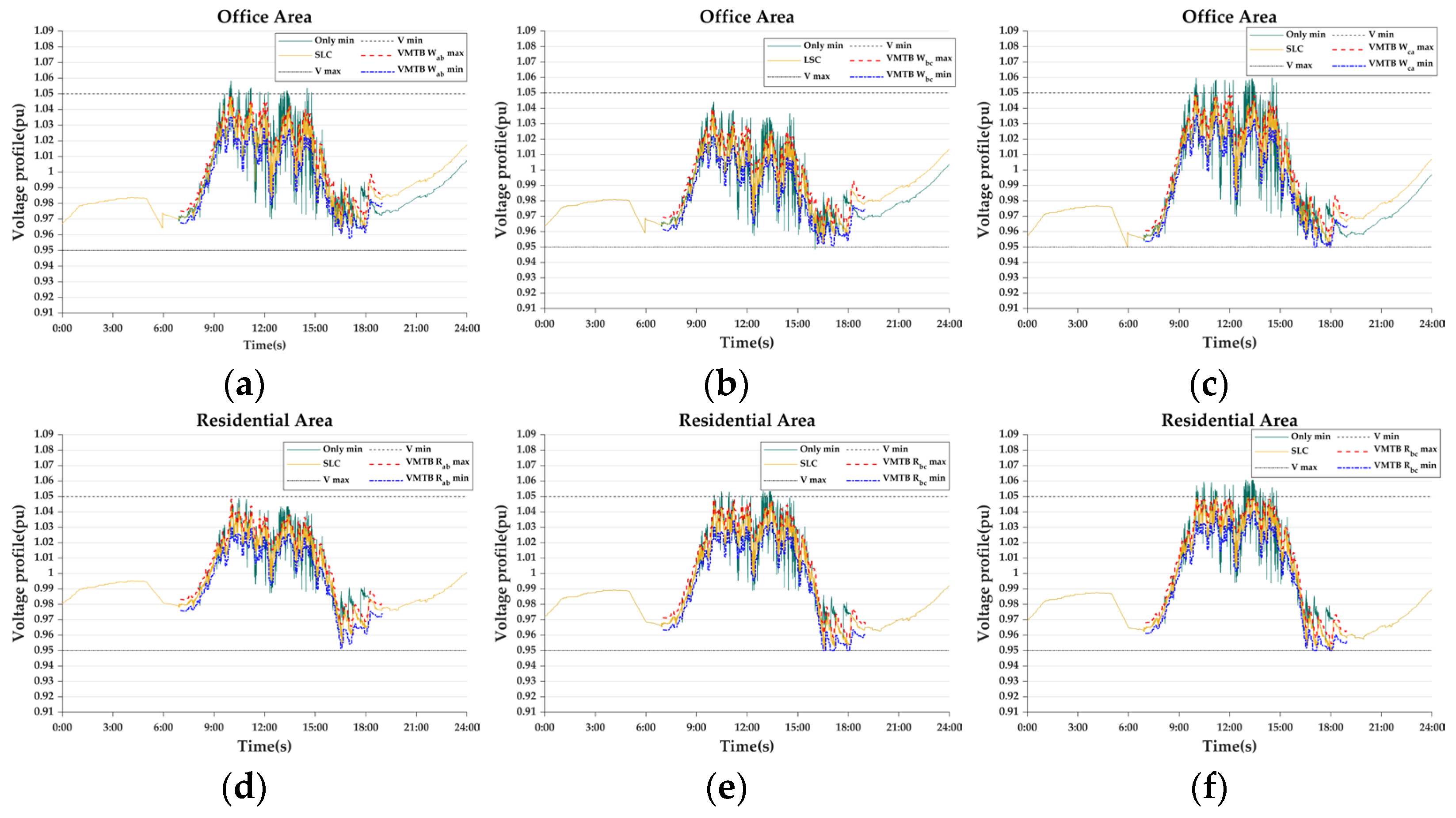
  • A novel vine model threshold band (VMTB) strategy is proposed to improve the frequent voltage fluctuations caused by the strong stochasticity of PV output.
  • A deviation optimization management (DOM) strategy based on SOC management is proposed to increase the available capacity of the DESS while avoiding deep charging/deep discharging of the DESS.
The structure of this paper is arranged as follows: Section 2 presents the mathematical models of various voltage regulation devices. Section 3 introduces the proposed spatio-temporal adaptive voltage coordinated control strategy. Section 4 performs simulations and analyzes the results. Finally, the conclusion is given in Section 5.

2. Mathematical Formulation
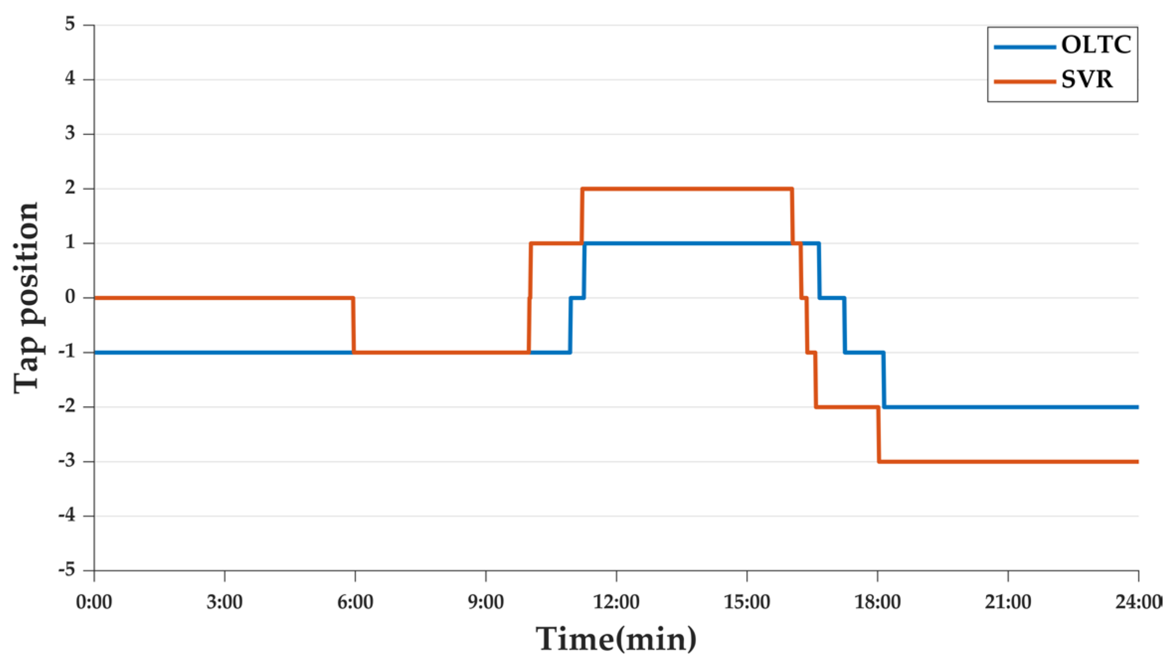
In this paper, the voltage regulation devices involved include the OLTC, SVR, DESS, and EVs. The mathematical model of each voltage regulation device is illustrated in this section.

2.1. OLTC

As a discrete voltage regulation device, the OLTC realizes discrete voltage regulation by changing the tap position. The relationship between the tap position change of the OLTC and the voltage is expressed in Equation (1) [36]:
Δ V tap oltc t = N tap oltc t N tap oltc t 1 · Δ v tap oltc
where Δ V tap oltc t is the voltage variation caused by the tap change of the OLTC at time t. N tap oltc t is the tap position of the OLTC at time t. Δ v tap oltc is the voltage step of each tap of the OLTC.
The constraint of the tap position of the OLTC is expressed in Equation (2):
  N _ tap oltc N tap oltc t   N - tap oltc
where N - tap oltc and   N _ tap oltc are the upper and lower limits of the OLTC tap position, respectively.

2.2. SVR

Although both the SVR and OLTC are discrete voltage regulation devices, the SVR is usually placed in the middle of the feeder and is used for the voltage regulation of feeders. The relationship between the tap position change of the SVR and the voltage is expressed in Equation (3) [36]:
Δ V tap svr t = N tap svr t N tap svr t 1 · Δ v tap svr
where Δ V tap svr t is the voltage variation caused by the tap change of the SVR at time t. N tap svr t is the tap position of the SVR at time t. Δ v tap svr is the voltage step of each tap of the SVR.
The constraint of the tap position of the SVR is expressed in Equation (4):
  N _ tap svr   N tap svr t     N - tap svr
where N - tap svr and N _ tap svr are the upper and lower limits of the SVR tap position, respectively.

2.3. DESS

As a continuous voltage regulation device, the DESS realizes continuous and precise voltage regulation by absorbing/releasing power to the DN. As an important parameter of the DESS, the SOC is not only the decision-making basis for DESS energy scheduling, but also a key parameter for DESS health management. The relationship between the SOC and power is given in Equation (5):
SOC t = SOC t 1 + n ϵ ϖ η bes ch P bes ch , n t + P bes dch , n t / η bes dch E bes Δ t
where SOC t and SOC t 1 are the SOC at time t and t 1, respectively. ϖ denotes phase ab, phase bc, and phase ca. P bes ch , n   and   P bes dch , n t   are the charging and discharging output of the DESS in phase n at time t.  E bes is the capacity of the DESS. η bes ch   and   η bes dch are the charging and discharging efficiencies of the DESS, respectively. Δ t is the time interval.
The constraints of the DESS charging and discharging power and SOC can be expressed as follows:
0     P bes ch , n t   P bes ch , max π ch , n t
  P bes dch , max π dch , n t     P bes dch , n t   0
SOC min SOC t SOC max
π ch , n t + π dch , n t 1 π ch , n t   a n d   π dch , n t 0 , 1
where   P bes ch , max   and   P bes dch , max are the maximum charging and discharging powers of the DESS, respectively. SOC max   and   SOC SOC are the upper and lower limits of the SOC. π ch , n t and π dch , n t are binary variables.

2.4. EVs

EVs can engage in voltage regulation of the DN via V2G technology. This study categorizes EVs into two modes, fast charging and slow charging, based on their distinct charging behaviors in individual functional areas. The charging power   P ev ch t and discharging power   P ev dch t of EVs at the EV power station at time t are represented in Equations (10) and (11):
P ev ch t = l = 1 L t η ev ch P ev , l ch - f t + y = 1 Y t η ev ch P ev , y ch - s t
P ev dch t = l = 1 L t P ev , l dch - f t / η ev dch + y = 1 Y t P ev , y dch - s t / η ev dch
where P ev , l ch - f t and P ev , l dch - f t are the fast-charging and fast-discharging powers of EV l at time t, respectively. P ev , y ch - s t and P ev , y dch - s t are the slow-charging and slow-discharging powers of EV y at time t, respectively. η ev ch and η ev dch represent the efficiency of EV charging and discharging.   L t and Y t are the total numbers of fast-charging and slow-charging EVs in the power station at time t, respectively.

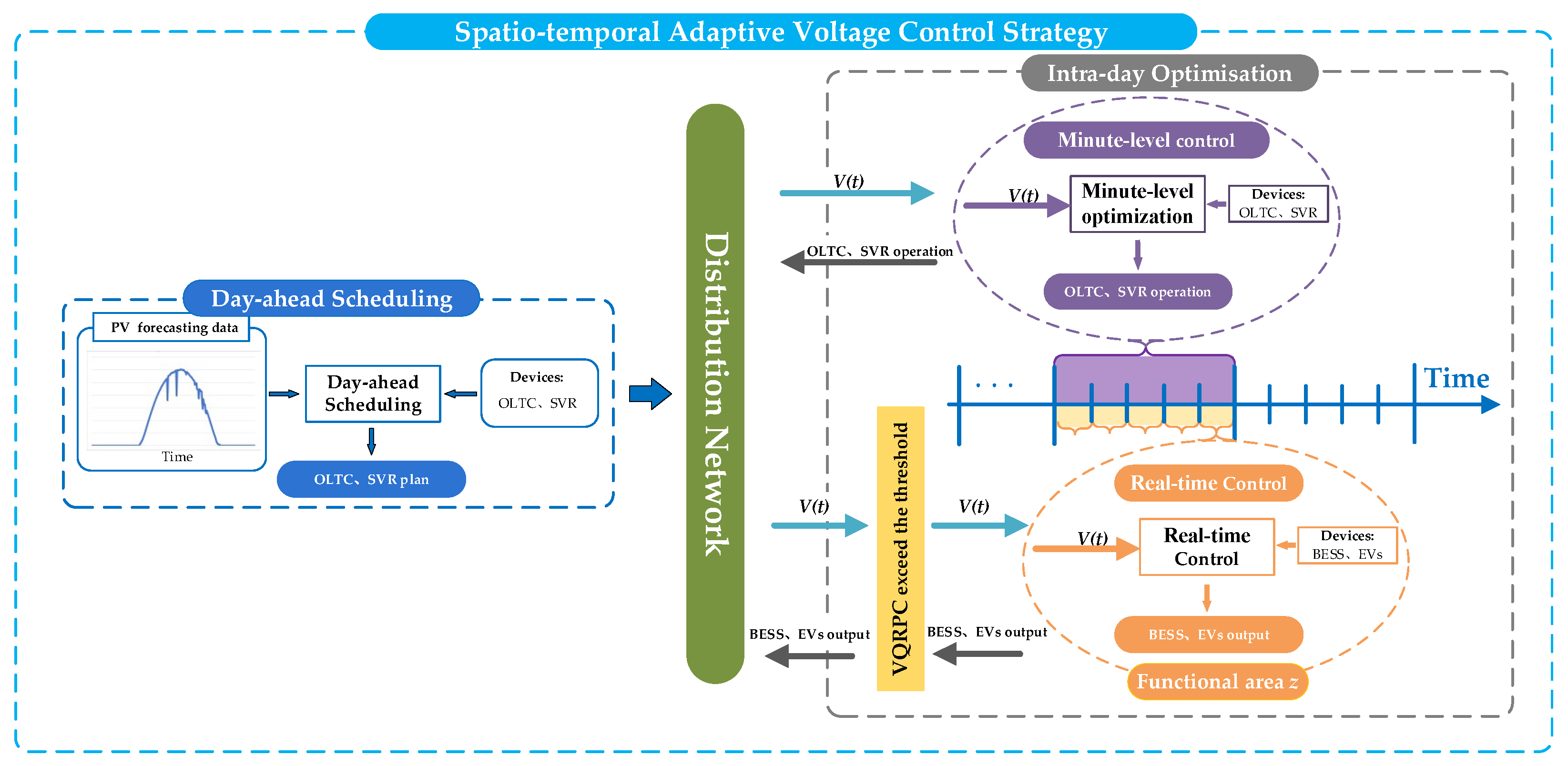
3. Spatio-Temporal Adaptive Voltage Coordination Control Strategy for Distribution Networks with High Photovoltaic Penetration

As the penetration rate of PVs in the DN is steadily increases, it can potentially lead to significant voltage violations. Facing the dual challenges of massive data collection demand and enhanced stochasticity on both the source and load sides in the new DN, an artificial intelligence or MPC control strategy is a more convenient strategy to realize voltage control [32,33,37], but it may face multiple challenges in communication, computation, and data storage. Therefore, this study innovatively proposes a coordinated voltage control architecture for DNs based on spatio-temporal coupling characteristics, aiming to realize complex scheduling through simple control means, improve the voltage quality of DNs, and reduce the workload of real-time data acquisition while balancing mechanical voltage regulators and power electronic voltage regulators. The strategy proposed in this paper is divided into day-ahead scheduling and intra-day optimization.

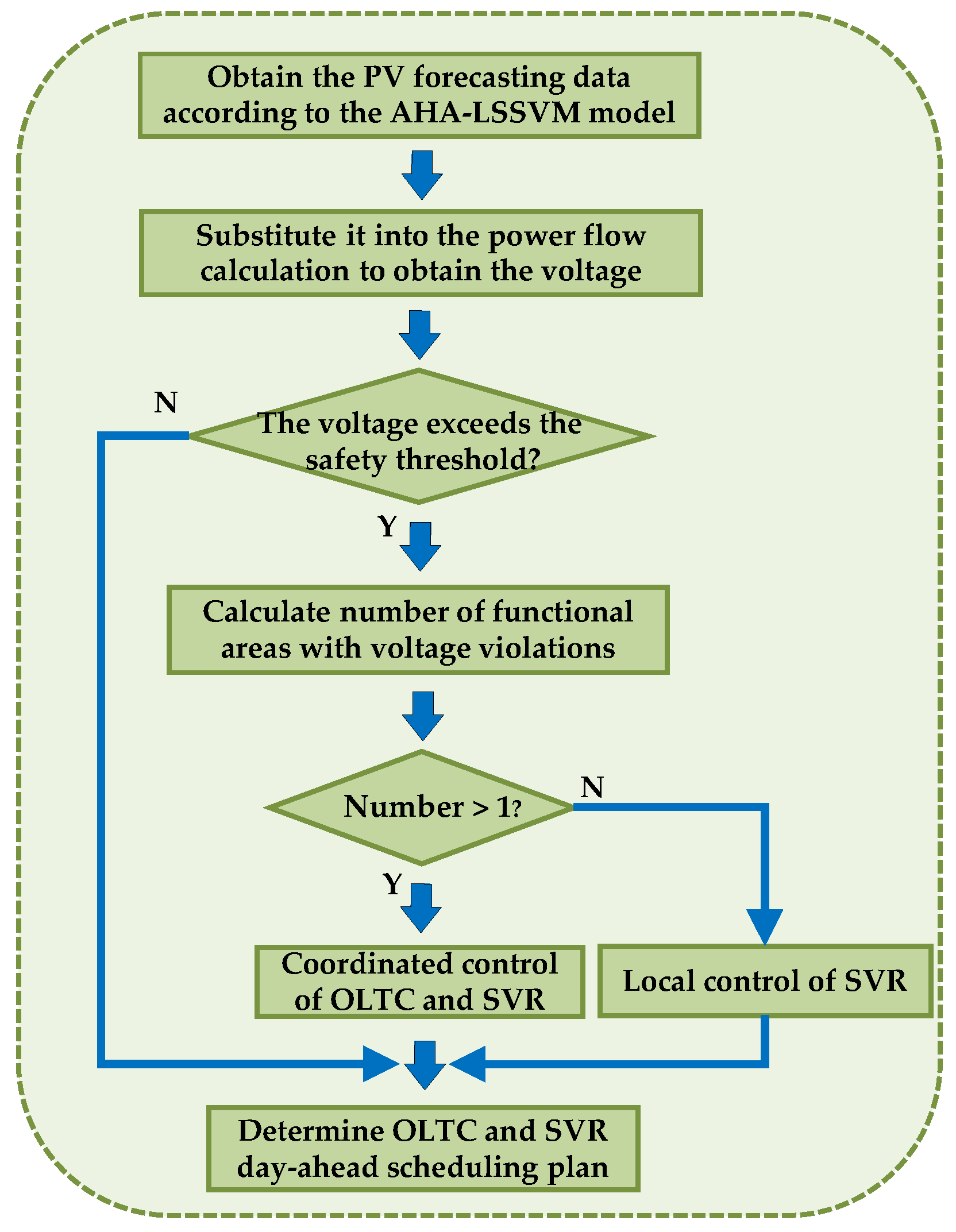
3.1. Day-Ahead Scheduling

In the day-ahead scheduling stage, the AHA-LSSVM PV forecasting model [38] is adopted, as proposed in our previous work (whose forecasting accuracy has been verified). This model is employed to generate the full-day PV output forecast profile. The day-ahead scheduling plans for the OLTC and SVR are then formulated based on the PV output from this model. The detailed process for OLTC and SVR day-ahead scheduling plan development is given in Appendix A. The flowchart of day-ahead scheduling is shown in Figure 1.

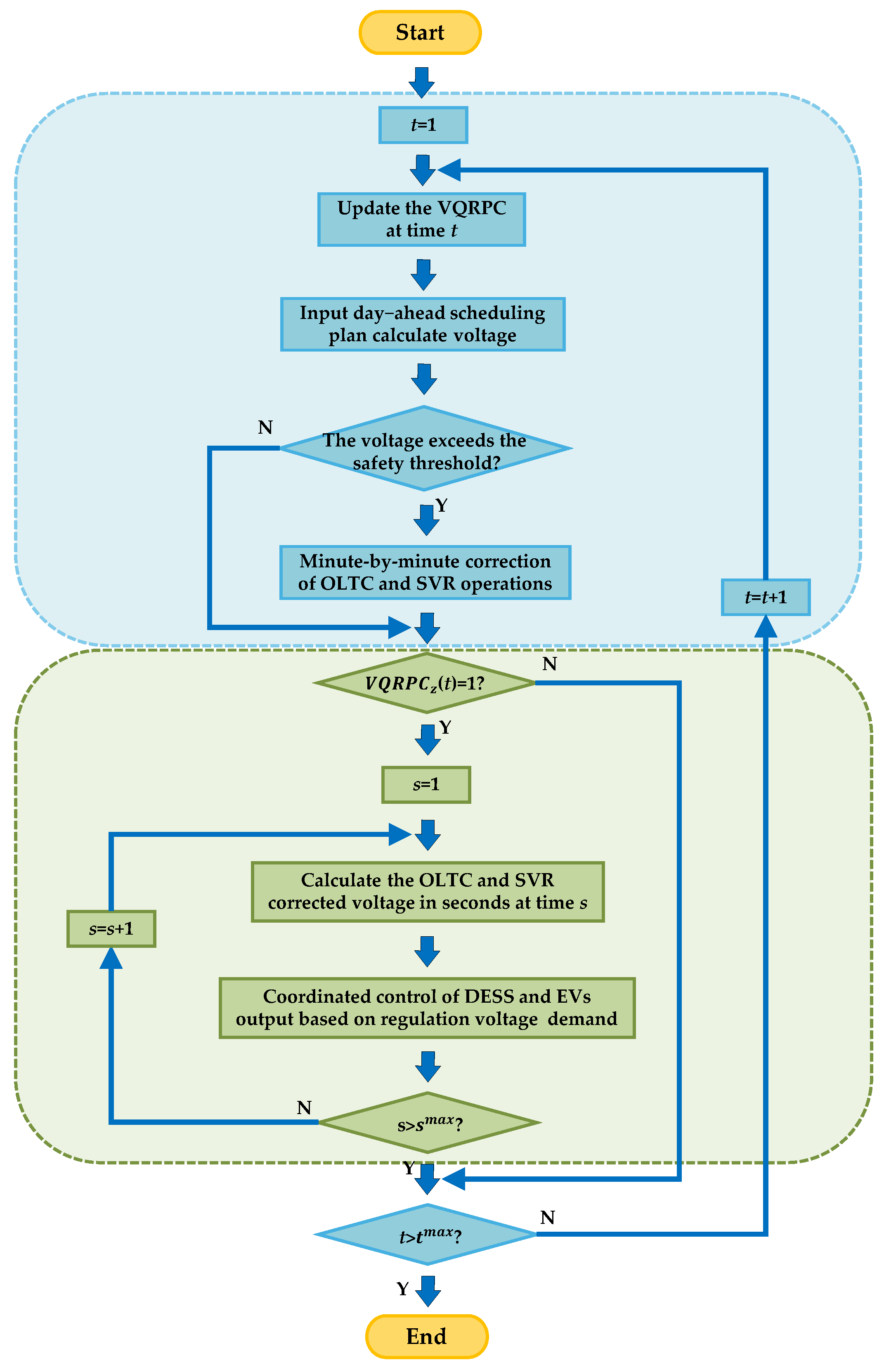
3.2. Intra-Day Optimization

For the intra-day optimization phase, this paper constructs a two-layer collaborative architecture of intra-day minute-level optimization and real-time adaptive control, as shown in Figure 2. Considering the strong randomness of PV output, the day-ahead scheduling plans of the OLTC and SVR are likely to lead to the deterioration of voltage quality and even the risk of voltage violation. Therefore, it is necessary to correct the day-ahead schedules of the OLTC and SVR at the minute level and to regulate the real-time voltage violation and fluctuations within the functional area by the regulation function of the DESS. In order to avoid the heavy workload caused by global real-time data collection, a real-time voltage quality assessment index, the VQRPC, is proposed as a criterion for switching the real-time control modes of each functional area.

3.2.1. VQRPC

In order to comprehensively measure the real-time voltage quality of each functional area, the VQRPC proposed in this paper consists of two parts. These are, respectively, the voltage amplitude risk prognostication coefficient (VARPC), used to measure the degree of voltage deviation in the functional area, and the voltage fluctuation risk prognostication coefficient (VFRPC), used to measure the intensity of voltage fluctuation in the functional area. The   VQRP C z t   + 1 of functional area z at time t + 1 is given in Equation (12).
  VQRP C z t + 1 = 1   i f   z vqrpc t + 1 > 0 0   e l s e
z vqrpc t + 1 = n ϵ ϖ VARPC z , dve   n t + 1 + n ϵ ϖ VFRPC z , flu   n t + 1   i f T st t T ed n ϵ ϖ VARPC z , dve   n t + 1   e l s e
where VARPC z , dve   n t   + 1 is the VARPC of phase n in functional area z at time t + 1. VFRPC z , flu   n t + 1 is the VFRPC of phase n in functional area z at time t + 1. T st and T ed are the start and end times of PV output. z vqrpc t   + 1 is the voltage quality index of functional area z at time t + 1. Considering that voltage fluctuations are mainly caused by the output of PVs, during the periods when PVs are not output, z vqrpc t   + 1 is only composed of the VARPC at time t + 1.
  • VARPC
In this paper, the VARPC is dynamically updated based on the short-term prediction of the autoregressive integrated moving average (ARIMA) model. Specifically, the voltages at ο sampling points from time t ο to time t are fitted, and the fitted voltages are used as inputs for the ARIMA model to predict the voltage of the functional area at the next moment, which is denoted as V z - i   pre , n t + 1 . And the maximum voltage deviation within the period from the time of t ο to the time of t is taken as the prediction error margin   Δ V z   er , n t + 1 at time t + 1. The VARPC of functional area z at time t + 1 is shown in Equation (14):
VARPC z , dve   n t + 1 = 1   i f   V z , ind max , n t + 1 > V   max   o r   V z , ind SOC , n t + 1 > V   SOC 0       e l s e
V z , ind   max , n t + 1 = max V z - i   pre , n t + 1 + Δ V z   er , n t + 1
V z , ind   SOC , n t + 1 = SOC V z - i   pre , n t + 1 Δ V z   er , n t + 1
Δ V z   er , n t + 1 = max V z - i n t ι V z - i n t ι 1 V nom , ι 0 , 1 , . . . , ο
where V z , ind   max , n t + 1 is the maximum value of the predicted voltage of phase n in functional area z at time t + 1. V z , ind   SOC , n t + 1 is the minimum value of the predicted voltage of phase n in functional area z at time t + 1. V z - i   n t ι is the voltage of phase n at node i in functional area z at time t ι . V nom is the rated voltage.
2.
VFRPC
During PV output time, due to the randomness of PV output, voltage in the DN will have frequent fluctuations, which adversely affect the stable operation of the DN. The VFRPC of functional area z at time t + 1 is shown in Equation (18):
VFRPC z , flu   n t + 1 = 1   i f   Δ V   z , flu max , n t + 1 > Δ V da avg , n 0   e l s e
Δ V   z , flu max , n t + 1 = max V z - i   pre , n t + 1 V z - i   n ( t )
Δ V da   avg , n = ϱ = T st T ed V i , da   n t ϱ V i , da   n t ϱ 1 V nom T ed - T st
where Δ V   z , flu max , n t + 1 is the maximum predicted voltage fluctuation of phase n in functional area z at time t + 1. Δ V da   avg , n is the upper limit of the voltage fluctuation threshold of phase n. V i , da   n t ϱ is the voltage of node i in phase n at time t ϱ .

3.2.2. Minute-Level Optimization

In minute-level optimization, the voltage V i , ind n t at time t is obtained through the day-ahead scheduling plans of the OLTC and SVR. When V i , ind   n t satisfies Equation (21), the OLTC and SVR maintain their current positions. Otherwise, the voltage Δ V z , ind t that needs to be regulated in each functional area at time t is calculated. The correction process of the OLTC and SVR at time t can be referred to in Section 3.1.
V   min V i , ind   n t     V   max
where V   max   and   V   min are the upper and lower limits of voltage, respectively.

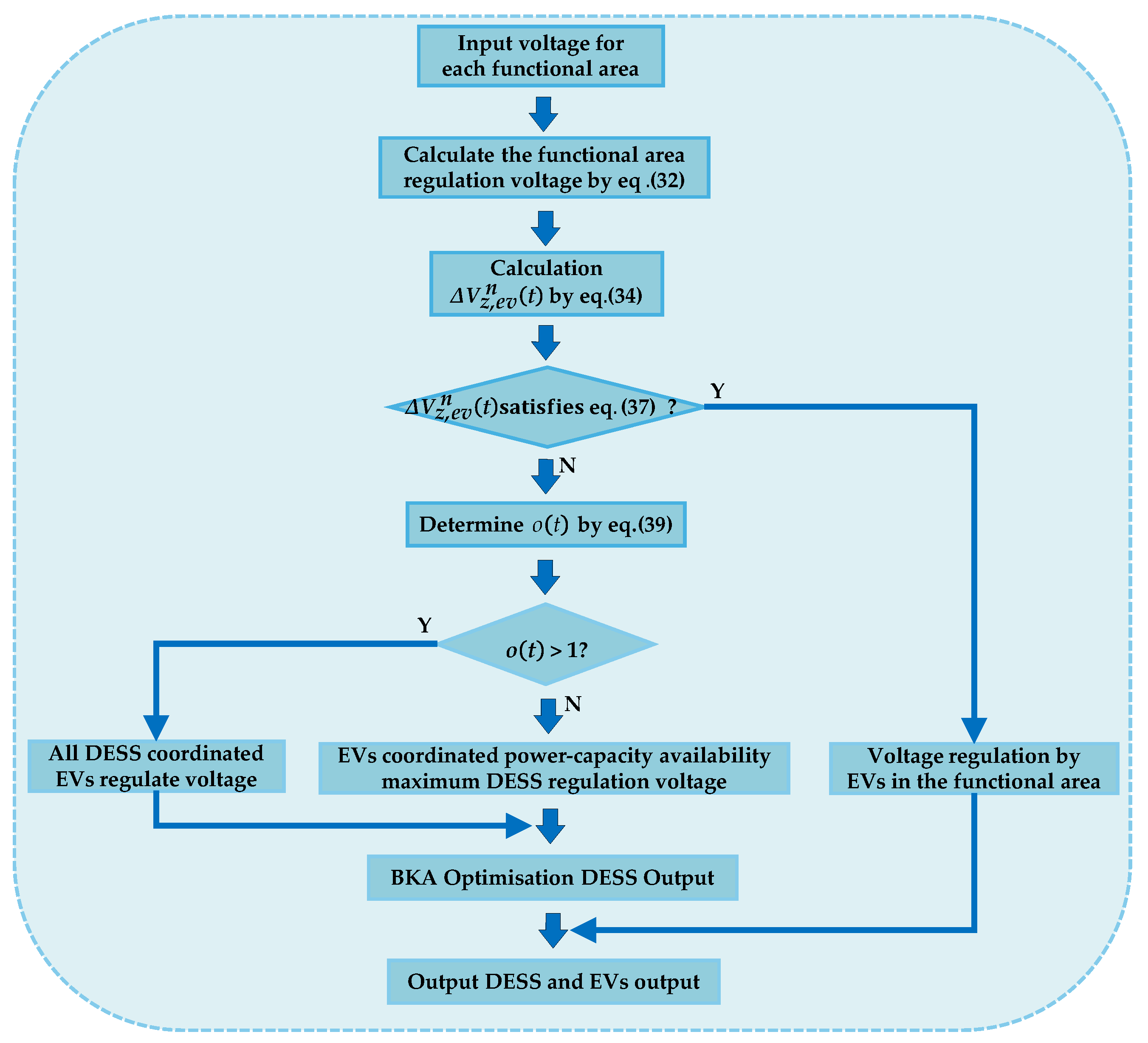
3.2.3. Real-Time Adaptive Control

When VQRP C z t = 1 is satisfied, it indicates that the strong randomness of PVs at time t may lead to voltage violations or fluctuations within functional area z, and functional area z enters real-time control. Through the coordinated control of the DESS and EVs, in combination with the global optimization of the OLTC and SVR, the real-time improvement of voltage quality within functional area z is achieved. Real-time control is further divided into voltage regulation mode, voltage fluctuation suppression–deviation optimization management (VFS-DOM) mode, and comprehensive optimization mode, according to the real-time voltage status, as shown in Equation (22):
M z t = 1   i f β z , r - v t > 0   and β z , r - f t = 0 2   i f β z , r - v t = 0   and β z , r - f t > 0 3   i f β z , r - v t > 0   and β z , r - f t > 0
β z , r - v t = n ϵ ϖ β z , r - v n t
  β z , r - v n t = 0   if   V   min >   V z - i , rea n t > V max 1   e l s e
  β z , r - f t = n ϵ ϖ β z , r - f n t
β z , r - f n t = 0   i f   m a x V z - i , rea n t V z - i , rea n t 1 > Δ V da avg , n 1   e l s e
where M z t is the mode of the DESS in functional area z at time t. β z , r - v t is the voltage regulation index in functional area z at time t. β z , r - f n t is the voltage fluctuation suppression index within functional area z at time t. V z - i , rea n t is the voltage of phase n at node i in functional area z at time t under real-time control.
After minute-level optimization, functional area z enters real-time control. Relying on the fast and accurate voltage regulation characteristics of the DESS, real-time voltage control is carried out. When M z t = 1 , it indicates that there is a voltage violation in functional area z. The DESS in functional area z switches to voltage regulation mode and quickly controls the voltage within the safe threshold. When M z t = 2 , it means that there is a problem of voltage fluctuations exceeding the threshold in functional area z. The DESS immediately enters VFS-DOM mode. While suppressing voltage fluctuations, it manages the SOC of the DESS. When M z t = 3 , it shows that while there is a voltage violation in functional area z, the voltage fluctuations also exceed the threshold. The DESS enters comprehensive optimization mode. It controls the voltage within the threshold and suppresses voltage fluctuations at the same time.
  • Voltage regulation mode
  • DESS Available Capacity Management Mechanism
Relying solely on the sensitivity index as the criterion for the output of the DESS will lead to a twofold problem. On the one hand, a DESS with high sensitivity in the functional area will accelerate the attenuation of its life cycle due to frequently undertaking charging and discharging tasks. On the other hand, a DESS with low sensitivity in the functional area will remain in a state of low utilization for a long time, resulting in the idleness of resources. In this study, a novel index of charging power–capacity availability J p c , b ch t and an index of discharging power–capacity availability J p - c , b dch t are proposed. These indices effectively coordinate the output of the DESS in the functional area by integrating the real-time available capacity and power availability of the DESS and improve the homogenization of the SOC in the functional area. J p - c , b ch t and J p - c , b dch t are represented in Equation (27) and Equation (28), respectively.
J p - c , b ch t = SOC max SOC b ( t ) ϱ bss , b ch ( t ) E bes , b
J p - c , b dch t = SOC b t SOC min ϱ bss , b dch ( t ) E bes , b
ϱ bss , b ch ( t ) = max S i , j V P · η bes ch P bes , b ch , max S i , j V P · η bes ch P bes , b ch , max
ϱ bss , b dch ( t ) = max S i , j V P · P bes , b dch , max / η bes dch S i , j V P · P bes , b dch , max / η bes dch
Δ P Δ Q = P θ P V Q θ Q V · Δ θ Δ V S i , j V P = V i P j = P V P θ · Q θ 1 · Q V 1
where ϱ bss , b ch ( t ) and ϱ bss , b ch ( t ) are the charging and discharging power availability of the bth DESS, respectively. S i , j V P is the function of active power and voltage. Δ P and Δ Q are the active and reactive power changes, respectively. Δ θ and Δ V are the phase angle and voltage amplitude changes, respectively. P θ , P V , Q θ , a n d   Q V are terms of the Jacobian matrix.
In this paper, a coordinated control strategy based on EVs in the functional area is proposed. By dispatching EVs within the functional area to participate in the voltage regulation of the DN, coordinated power output with the DESS is achieved. This effectively reduces the capacity requirement of the DESS. In particular, to achieve precise voltage regulation with the DESS in the functional area, this paper adopts the recently proposed BKA to optimize the power output of the DESS [39]. This algorithm simulates the dynamic encirclement strategy of the black-winged kite during predation and attack, as well as the highly adaptive and intelligent behavior demonstrated during its migration process. It has the characteristics of strong adaptability, few adjustable parameters, and high convergence accuracy [40,41]. The specific implementation steps are as follows.
Step 1: Determine whether the voltage V z - i , rea n t in functional area z satisfies Equation (21); if not, calculate the voltage Δ V z - i , rea n t to be regulated according to Equation (32).
Δ V z - i , rea n t = V z - i , rea n t V max   i f ρ z n t = 1   V z - i , rea n t V min   i f ρ z n t = 1 0   e l s e
ρ z n t = 1   i f   V z - i , rea n t > V max 1   i f   V z - i , rea n t > V min 0   e l s e
where ρ z n t is an indicator of n phase voltage violation in functional area z at time t.
Step 2: Calculate the regulated voltage Δ V z , ev n t of EVs in functional area z at time t according to Equation (34), and, if Equation (37) is satisfied, then voltage regulation ends at time t, and only EVs in functional area z are used to regulate the voltage. Otherwise, proceed to step 3, using the DESS and EVs to execute coordinated control.
Δ V z , ev n t = S i , j V P · P z , ev ch , n t   i f ρ z n t > 0 S i , j V P · P z , ev dch , n t   i f ρ z n t < 0
P z , ev ch , n t = l = 1 L z t η ev ch P ev , l ch - f , n t + y = 1 Y z t η ev ch P ev , y ch - s , n t
P z , ev dch , n t = l = 1 L z t P ev , l dch - f , n t / η ev dch t + y = 1 Y z t P ev , y dch - s , n t / η ev dch t
Δ V z , ev n t   >   Δ V z - i , rea n t
where P z , ev ch , n t and P z , ev dch , n t are the dispatchable EVs’ n phase charging and discharging power in functional area z at time t, respectively. L z t and Y z t are the number of EV fast- and slow-charging numbers that can be dispatched in functional area z at time t.
Step 3: Calculate the voltage V z - i , rea   re , n t of functional area z after the regulation of EVs at time t according to Equation (38), and calculate the voltage Δ V z - i , rea re , n t required for coordinated control of the DESS in the functional areas according to Equation (32).
V z - i , rea   re , n t = V z - i , rea n t Δ V z , ev n t
Step 4: Determine the number ο t of DESSs participating in voltage regulation in functional area z at time t according to Equation (39); if   ο t = 1 indicates economic voltage regulation, only the DESS with the highest power–capacity availability in functional area z is required to participate in voltage regulation. Otherwise, emergency co-regulation is required, and all the DESSs in functional area z co-ordinate to control the voltage.
  ο t = 1   i f   Δ V bse , z min m a x V z - i , real n , re t B z e l s e
  Δ V bse , z min = min S i , j V P · P bes , b max ,   b ϵ ( 0 , 1 , , B z )
where Δ V bse , z min is the threshold for economic voltage regulation in functional area z. P bes , b max is the maximum output of the bth DESS in functional area z.  B z is the number of DESSs in functional area z.
Step 5: Determine the BKA variable dimension ξ z t according to Equation (41) and set the upper and lower boundaries, number of iterations, and population parameters to randomly initialize the black-winged kite position.
ξ z t = n ϵ ϖ ξ z n t
ξ z n t = 0   i f   V min V z - i , rea n , re t V max ο t   e l s e
where ξ z n t is the number of DESS outputs in functional area z at time t.
Step 6: Calculate the fitness value f bka of the black-winged kite according to Equation (43) and select the individual with the best fitness value as the leader.
f bka = V max V z , bka max t   i f   V z - i , rea n , re t > V max V z , bka min t V min   i f   V z - i , rea n , re t > V min
where V z , bka   max t and V z , bka   min t are the maximum and minimum voltage in functional area z after bringing in the position of the black-winged kite, respectively.
If the voltage after bringing in the position of the black-winged kite does not satisfy Equation (21), then update it according to Equation (44).
f bka = f bka + k pen
where k pen is the penalty.
Step 7: Update the location of black-winged kites based on their unique attack and migration behavior [39].
Step 8: Repeat steps 6–7 until the maximum number of iterations is reached and the optimal black-winged kite position is output, that is, the optimal output P b , bka t of each DESS under voltage control.
The voltage regulation flowchart is shown in Figure 3.
2.
VFS-DOM mode
Considering the significant correlation characteristics between the life-cycle decay of the DESS and the depth of charging and discharging [42,43,44], this paper proposes the deviation degree ψ b t of the SOC to indicate the degree of SOC deviation from the expected SOC. When ψ b t of the DESS satisfies Equation (46), the DESS switches to voltage fluctuation suppression (VFS) mode to suppress voltage fluctuation; otherwise, it triggers the depth charging and discharging protection mechanism and switches to deviation degree optimization management (DOM) mode. By selectively suppressing the voltage fluctuation, ψ b t returns to the safety threshold, effectively avoiding the life-cycle decay triggered by deep charging and discharging of the DESS. ψ b t of the DESS at time t is expressed in Equation (45):
ψ b t = SOC b t SOC ex t SOC max SOC min
ψ min     ψ b t     ψ max
where ψ max and ψ min are the upper and lower limits of the degree of deviation, respectively. SOC ex t is the expected DESS SOC at time t. SOC b t is the SOC of the bth DESS at time t.
Considering that the DESS is in the charging state during the PV output rise stage, the SOC is maintained at a high level, while after the PV output peak, the DESS enters the discharging state and the SOC is at a relatively low level. Therefore, the variation in SOC ex t of the DESS with PV peak time T peak is given in Equation (47):
  SOC ex t = SOC ex , l   i f   t T peak SOC ex , h   i f   t > T peak
where SOC ex , l and SOC ex , h are the expected SOC before and after the PV peak.
  • VFS mode
The randomness of PV easily leads to frequent voltage fluctuations in the DN, which seriously affects the stability of system operation. In this paper, when the functional area M z t = 2 and ψ b t satisfies Equation (45), the DESS switches to VFS mode to suppress voltage fluctuation and improve the voltage quality of the DN. Considering that the voltage fluctuations are caused by PV output, the constraint on the time period T for smoothing out voltage fluctuations is given in Equation (48).
T st     T vfs     T ed
  • VMTB
In this paper, the suppression of voltage fluctuation in the functional area is achieved with the VMTB, which is defined as shown in Equations (49)–(51):
V vm , z max , n t + 1 = V z pre , n t + 1 + Δ V z , vm n t + 1
V vm , z min , n t + 1 = V z pre , n t + 1 Δ V z , vm n t + 1
Δ V z , vm n t + 1 = max α 1 Δ V da   avg , n + α 2 Δ V z - i , lts avg , n t + 1
  Δ V z - i , lts avg , n t + 1 = d = 0 ο V z - i , lts   n t d ο
  α 1 + α 2 = 1 α 1 , α 2 0 , 1
where V vm , z   max , n t   + 1 and V vm , z   min , n t   + 1 are the upper and lower limits of the VMTB at time t + 1, respectively. V z   pre , n t   + 1 is the n phase ARIMA-predicted voltage in functional area z at time t + 1.   Δ V z , vm   n t   + 1 is the safety margin for voltage fluctuations in the functional area z at time t + 1.   Δ V z - i , lts avg , n t   + 1 is the average of n phase voltage fluctuations at node i of functional area z from time period t to t ο . α 1 and α 2 are constants.
If the VMTB exceeds the safety threshold for overvoltage, then the VMTB is updated according to Equation (54):
V vm , z max , n t + 1 = V max       i f   V vm , z max , n t + 1 > V max V vm , z min , n t + 1 = V min       i f   V vm , z min , n t + 1 < V min
The flowchart of the VMTB for suppressing voltage fluctuation is shown in Figure 4, and the steps are as follows.
Step 1: Calculate the voltage fluctuation   Δ V z , vfs   n t to be smoothed at time t according to Equation (55)
  Δ V z , vfs   n t = Δ V z n , u t + Δ V z n , l t
    Δ V z n , u t = V z , rea n t V z , vm max , n t                             i f   V z , rea n t > V z , vm max , n t 0 i f V z , rea n t V z , vm max , n t
Δ V z n , l t = V z , rea n t V z , vm min , n t                             i f   V z , rea n t > V z , vm min , n t 0 i f V z , rea n t V z , vm SOC , n t
where Δ V z n , u t   and   Δ V z n , l t   are the deviations of n phase voltages in functional area z from the upper and lower limits of the VMTB at time t, respectively.
Step 2: Calculate EV voltage regulation Δ V z , ev   n t in functional area z at time t according to Equation (58):
  Δ V z , ev   n t = S i , j V P · P z , ev n , ch t   i f   Δ V z , vfs n t > 0 S i , j V P · P z , ev n , dch t   i f   Δ V z , vfs n t > 0
Step 3: If Equation (59) is satisfied, then proceed to step 4 to suppress voltage fluctuations using only EVs; otherwise, proceed to step 5 where the DESS is used to coordinate EVs to suppress voltage fluctuations.
Δ V z , ev   n t Δ V z , vfs   n t
Step 4: Calculate EV output   P z , ev n t according to Equation (60):
P z , ev n t = S i , j VP Δ V z , vfs   n t
Step 5: Use the DESS to coordinate EVs to suppress voltage fluctuation   Δ V z , bss n , re t according to Equation (61) and calculate the deviation ψ b t of the DESS in functional area z at time t according to Equation (45), where ψ b t is changed into the weight Γ b t of each DESS output in the functional area z at time t through Equations (62) and (63), and finally, the output P bes , b n t of each DESS is given by Equation (64):
  Δ V z , bss n , re t = Δ V z , vfs   n t Δ V ev , z   n t
  Υ b t = 1 ψ b t b B z ψ b t   i f   Δ V z , vfs n t > 0 1 + ψ b t b B z ψ b t   i f   Δ V z , vfs n t > 0
  Γ b t = Υ b t b B z Υ b t
  P bes , b n t = S i , j V P 1 / B z + Γ b t 2 Δ V z , bss n , re t
Check whether A satisfies Equation (65); if not, adjust A according to Equation (66):
  P bes dch , max     P bes , b n t     P bes ch , max
P bes , b n t = P bes dch , max   i f P bes , b n t < P bes dch , max P bes , b n t = P bes ch , max   i f P bes , b n t > P bes ch , max
  • DOM mode
When ψ b t of the DESS in functional area z does not satisfy Equation (46), it indicates that the significant deviation of the DESS as a whole from   SOC ex t in functional area z at the time t may lead to deep charging/deep discharging of the DESS; at this time, the DESS is switched to DOM mode, which selectively suppresses voltage fluctuation in the functional area through the DESS, while avoiding the life-cycle decay of the DESS due to deep charging/deep discharging.
  • VMTB adjustment
In the control strategy proposed in this paper, when the deviation ψ b t of DESS exceeds the upper limit threshold ψ max , the system will increase the lower limit of the VMTB according to Equation (68), which effectively suppresses the DESS deep charging risk triggered by excessive SOC deviation by increasing Δ V z n , l t . On the contrary, when ψ b t is lower than the lower limit threshold ψ SOC , it will decrease the upper limit of the VMTB according to Equation (67), thus mitigating the DESS deep discharge risk.
V z , vm - r max , n t = V z , vm max , n t k vfs Δ V z , vm n t
V z , vm - r min , n t = V z , vm min , n t + k vfs Δ V z , vm n t
where V z , vm - r max , n t and V z , vm - r   min , n t are the upper and lower adjusted VMTB limits. k vfs is the constant.
3.
Comprehensive optimization mode
When M z t = 3 , which indicates that both voltage violation and voltage fluctuation values exceed the threshold in functional area z, the DESS switches to comprehensive optimization mode, which suppresses voltage fluctuation while constraining voltage magnitude within the threshold.
The process of regulating voltage violations in comprehensive optimization mode can be referred to as voltage regulation mode, which, in the BKA optimization algorithm, differs in the design of the individual fitness function, manifested in the fact that comprehensive optimization mode adopts the composite fitness function shown in Equation (69), which integrates the demand for regulating the voltage with the demand for voltage fluctuation suppression, while the voltage regulation mode adopts the fitness function shown in Equation (43). The process of voltage fluctuation suppression in comprehensive optimization mode control is the same as in VFS-DM mode.
f bka - s = V z , vm max , n t V z , bka max t   i f   V z - i , real n , re t > V max V z , bka min t V z , vm min , n t   i f   V z - i , real n , re t < V min
where f bka - s is the value of the individual fitness function of the BKA optimization in comprehensive optimization mode.
In this paper, we propose a spatio-temporal adaptive voltage control strategy utilizing coordinated control of the OLTC, SVR, BESS, and EVs at different timescales and functional areas, and the control framework is shown in Figure 5. In day-ahead scheduling, the AHA-LSSVM forecasting model is used to obtain PV forecasting data, and the day-ahead scheduling plans for the OLTC and SVR are formulated. The day-ahead scheduling plans for the OLTC and SVR are optimized at the minute and intra-day levels. For real-time adaptive control, a zonal decision-making mechanism is adopted. When the VQRPC of functional area z exceeds the threshold value, functional area z enters real-time control mode, and the DESS and EVs respond rapidly for precise adjustment. Through this flexible voltage adjustment strategy, while improving the voltage quality, the workload of real-time data collection is effectively reduced.

4. Case Study

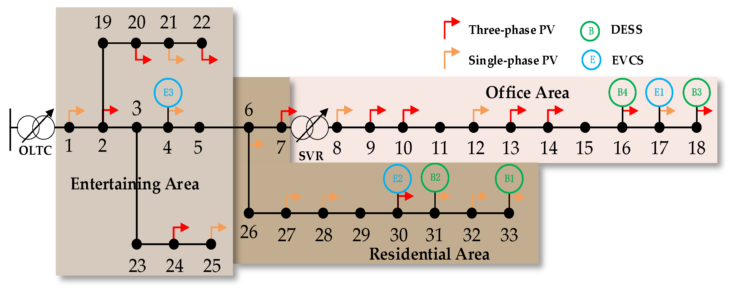
4.1. Simulation Conditions

In this paper, numerical simulations were carried out in the compilation environment of MATLAB 2022b and ran on a computer equipped with a 13th-generation Intel (R) Core (TM) i9-13900K processor with a frequency of 3.0 GHz and 32 GB DDR5-6400 of RAM, running on the Windows 11 Pro 22H2 operating system, with a modified IEEE 33 system selected as the simulation verification platform and the division of its functional areas shown in Figure 6. Based on the differences in travel behaviors of EVs, this system is divided into an office area, a residential area, and an entertainment area. The parameters of the modified IEEE 33 system are shown in Table 1, Table 2, and Table 3, respectively.
In this study, a spatio-temporal probabilistic model of EV charging loads in different functional areas is constructed based on the Monte Carlo random sampling method [45,46,47]. Based on the real-time status of EVs in the charging station, they are categorized into charging and idle states. When EVs are charging, they are connected to the DN as electric loads, while EVs in the idle state are regarded as virtual energy storage and regulated according to the voltage regulation demand of the DN in cooperation with the DESS. The modelling of EV charging behavior in each functional area follows the following principles:
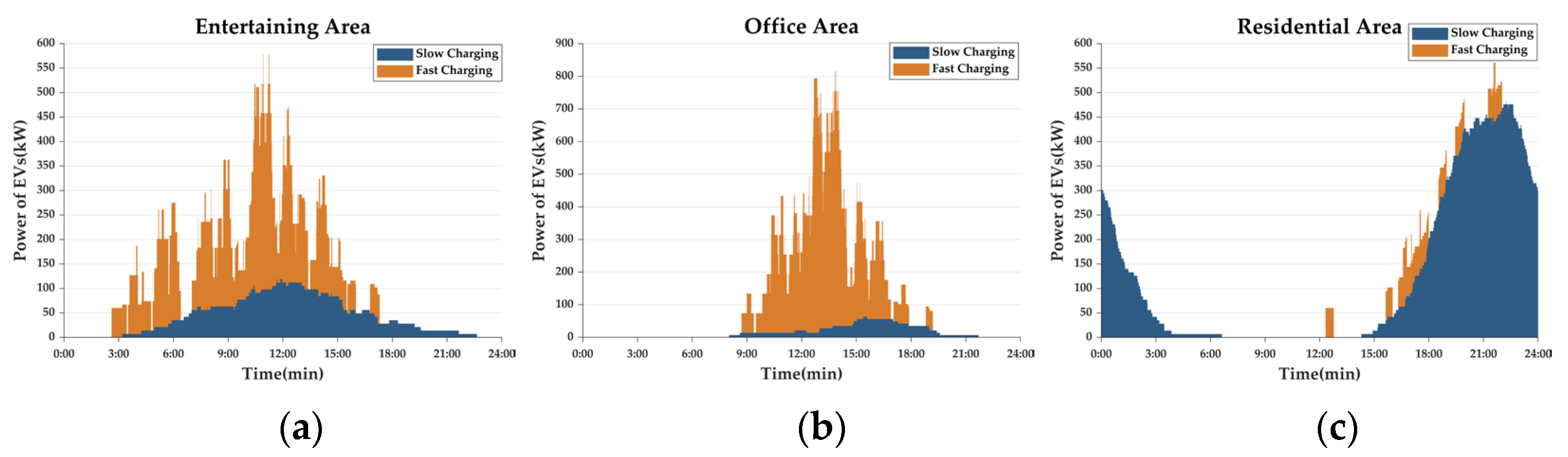
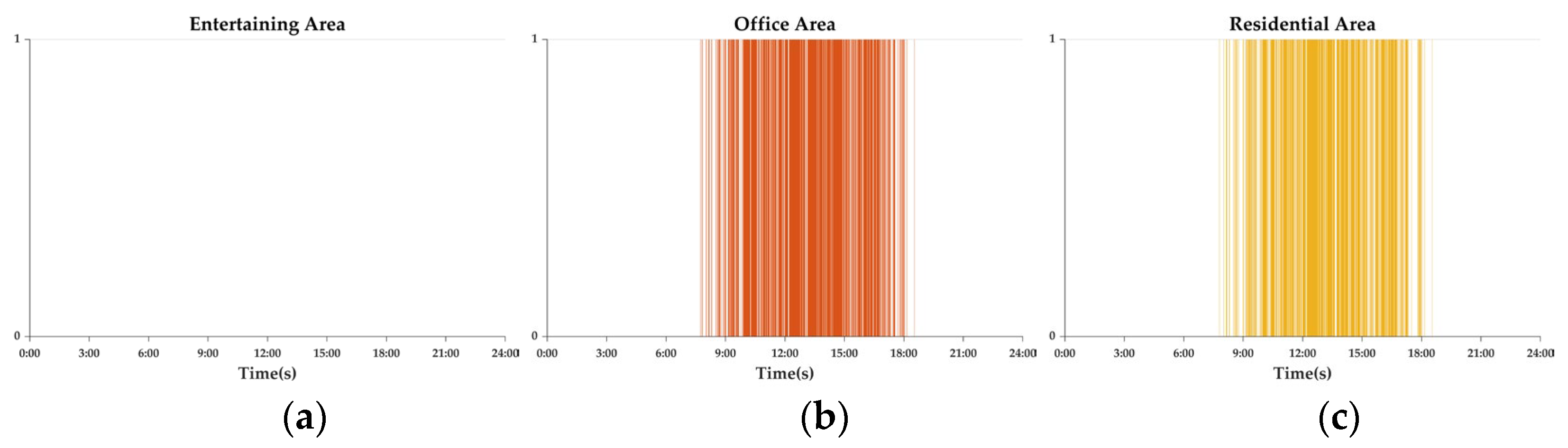
  • It is assumed that a total of 100 EVs are charging at the EV station in the functional area throughout the day and that the number of idle EVs is equal to the number of charging EVs in real time.
  • Referring to the 2022 China electric vehicle user charging behavior white paper [48], the fast- and slow-charging ratios for office, residential and entertainment areas are set at 9:1, 1:9 and 7:3, respectively.
  • The charging start time follows a normal distribution differentiated by the functional area, with office areas concentrated in the late afternoon N ( 13 ,   2 2 ) , residential areas peaking in the evening N ( 21 ,   2 2 ) , and entertainment areas showing a tendency to charge all day during the day ( 10 ,   3 2 ) .
Figure 7 shows the power of EVs charged at charging stations in each functional area.
In this paper, the AHA-LSSVM PV forecasting model is used to forecast the future PV output for the whole day, and Figure 8 shows the forecasting results of the AHA-LSSVM under cloudy weather.
From Figure 8, it can be seen that the AHA-LSSVM PV forecasting model has an excellent capability of dynamic tracking in PV forecasting. In terms of data, the mean absolute error (MAE) of the AHA-LSSVM is only 1.73%, and the root mean square error (RMSE) is 2.42%. The data show that the AHA-LSSVM has a significant advantage in PV forecasting accuracy and is able to forecast PV output more accurately.

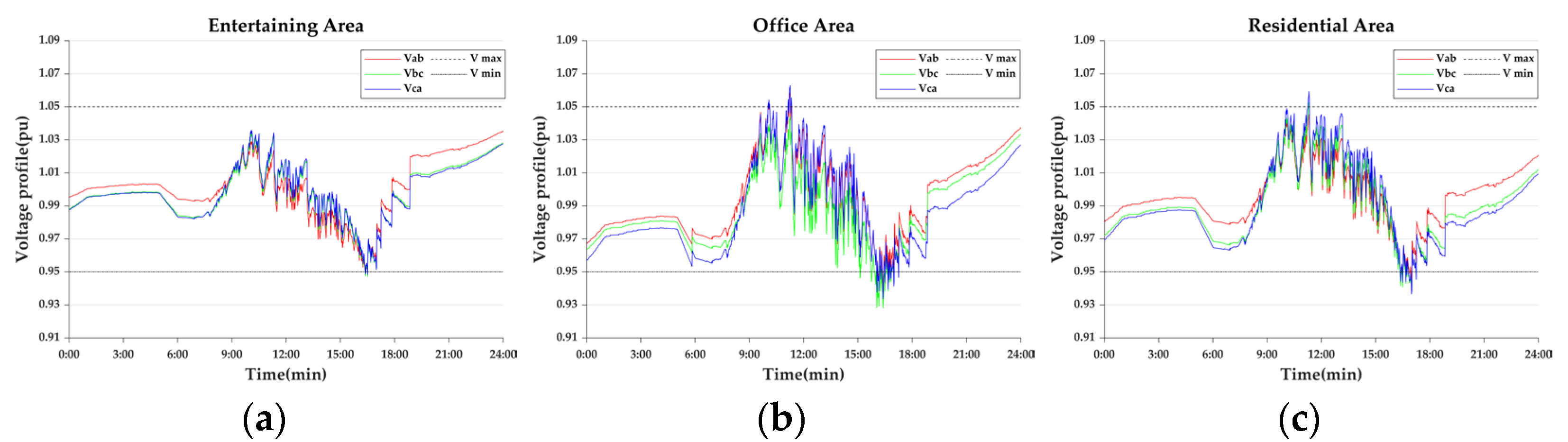
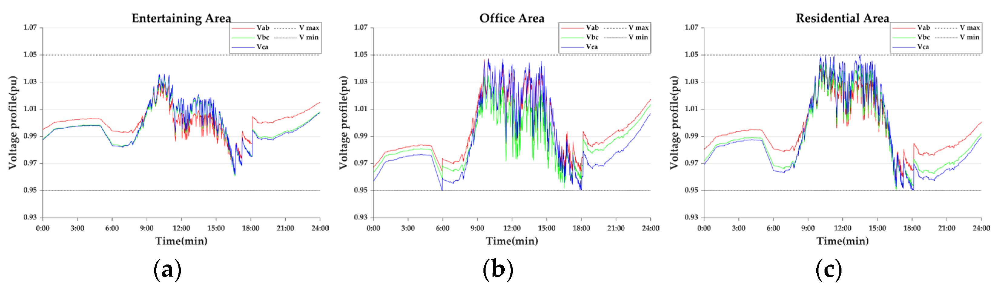
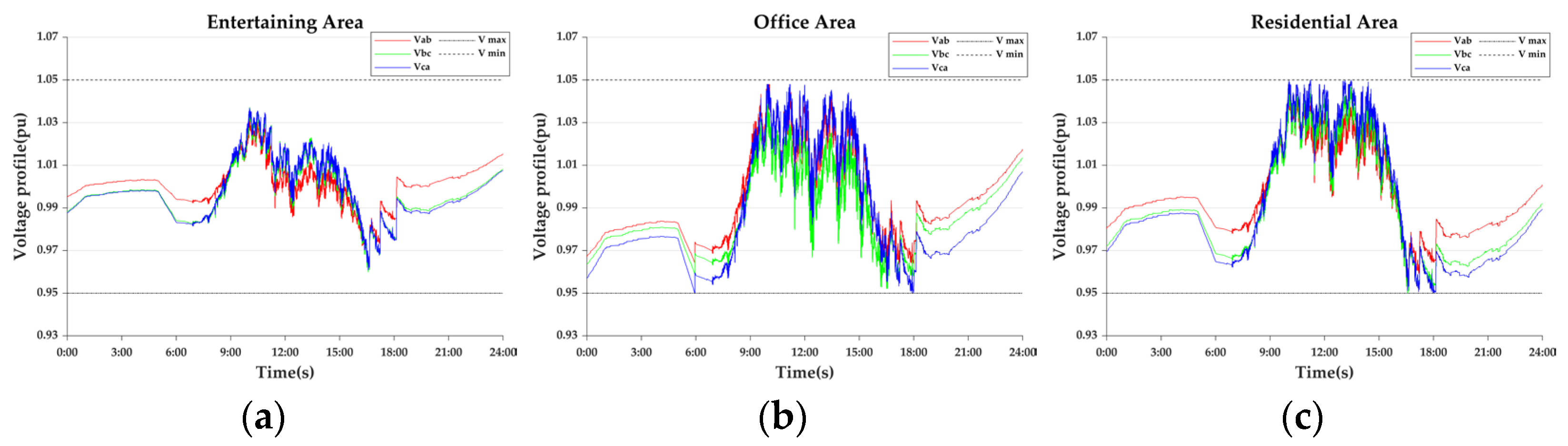
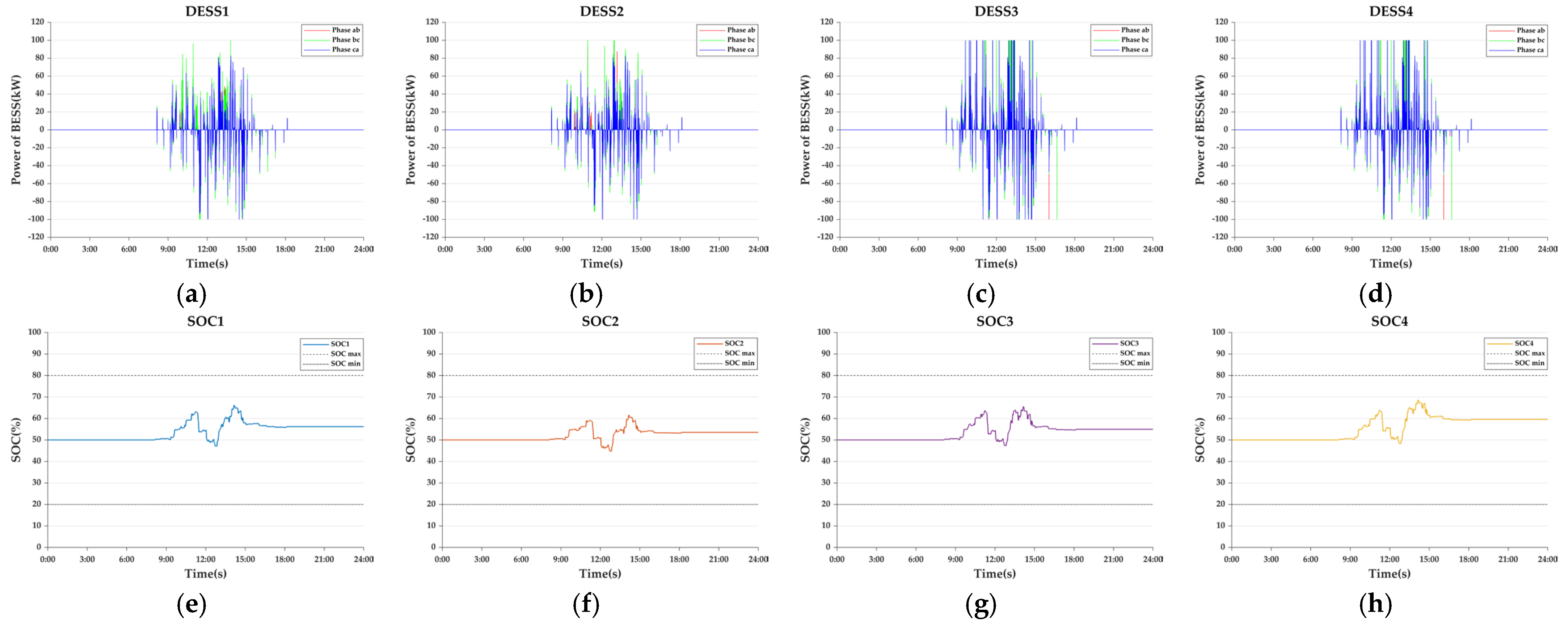
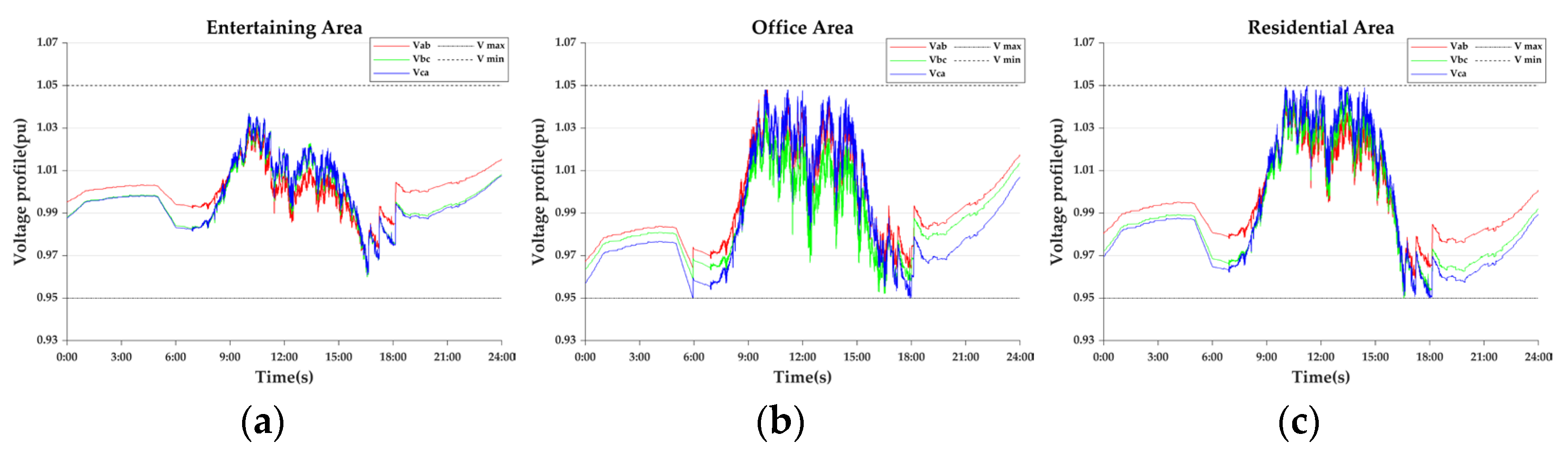
4.2. Case Study and Discussion

In order to analyze and verify the feasibility and effectiveness of the proposed spatio-temporal adaptive voltage coordination control strategy in improving voltage quality, a total of nine cases are designed in this paper, as shown in Table 4.
  • Day-ahead scheduling stage (5 min)
In Case 1-1, the AHA-LSSVM is used to forecast PV output, and forecast results are substituted into the current calculation to obtain the original voltage of each functional area in the day ahead. In Case 1-2, the OLTC and SVR optimization strategies proposed in this paper are used to globally optimize the voltages of each functional area in Case 1-1 and to verify the validity of the proposed strategies.
  • Intra-day optimization stage
Intra-day optimization is further divided into a minute and real-time level on the timescales of control.
  • Minute timescale (1 min)
Case 2-1 uses the OLTC and SVR day-ahead scheduling plans of Case 1-2 for intra-day optimization to verify the effectiveness of the strategy on an intra-day basis. Case 2-2 optimizes the day-ahead scheduling plan of Case 1-2 on a minute-by-minute level to confirm the necessity of correcting the day-ahead plan on an intra-day basis.
  • Real-time (10 s)
In Case 2-3, the optimized strategy in Case 2-2 is applied to the second-level timescale to further explore the feasibility and effectiveness of this strategy. In Case 2-4, real-time control is adopted. The DESS within the functional area adjusts the voltage locally under the optimization of the BKA, and suppresses voltage fluctuations through the VMTB. In Case 2-5, an adaptive real-time control strategy is implemented, which not only improves the voltage quality of the functional area but also reduces the workload of real-time data collection. In Case 2-6, the DOM strategy is adopted to alleviate the deep charging/discharging situations of the DESS and optimize the available capacity of the DESS. In Case 2-7, EVs are used to coordinate the control of the DESS, alleviating the pressure of DESS capacity configuration.
  • Case 1-1: The Original Day-ahead Voltage
In this paper, Nodes 5, 18, and 33 are selected as the key nodes for the entertainment, residential, and office areas respectively. The original voltage curves of each functional area are shown in Figure 9.
As shown in Figure 9, there are different degrees of voltage violations in each functional area. Comparing Figure 9b with Figure 9c, it is obvious that during the period from 12:30 to 15:30, there is a serious phenomenon of fast-charging EVs being connected in the office area. This situation leads to a significant difference in the voltage curves between the office area and the residential area, which highlights the importance and urgency of dividing the functional areas and implementing the zoning control strategy.
Due to the ordinary loads and EVs charging demand, combined with the lack of or low PV output, the voltage exceeds the lower limit in the residential area during 5:00–8:30 and 17:00–1:00 with a voltage minimum of 0.896 pu. Similarly, the entertainment area is exceeded in the entertainment area during 18:30–21:00, and the office area is exceeded in the office area during 5:30–8:00 and 17:00–0:30, with a voltage minimums of 0.947 pu and 0.917 pu, respectively.
As the PV output increases, the voltage exceeds the upper limit in the residential area during 11:00–15:30 and in the office area during 11:00–15:00, with the maximum values of 1.084 pu and 1.068 pu, respectively. no voltage exceeding the upper limit occurs in the entertainment area.
  • Case 1-2: Day-ahead Scheduling
As shown in Figure 10, the day-ahead scheduling plan successfully controls the voltage in each functional area within the safety threshold. This shows the effectiveness of the strategy proposed in this paper. The operation of OLTC and SVR in the day-ahead optimisation strategy is shown in Figure 11.
In Figure 11, the operations of OLTC and SVR are in accordance with the day-ahead scheduling plan, and at 0:00 h, both office and residential areas cross the lower limit at the same time, and OLTC has priority action to regulate the voltage of the whole distribution network. At 5:55, only the residential area is exceeding the lower limit, and the SVR has priority action to regulate the voltage of the localised residential area.
  • Case 2-1: Intra-day-day-ahead optimisation
After the day-ahead scheduling plan is implemented at the intraday minute level, the voltage profile of each functional area is shown in Figure 12.
From Figure 12, it can be seen that voltage violation still exists in residential and office areas after intraday execution of the day-ahead scheduling plan. This is due to the error between the actual PV output and the predicted value, and it is difficult to control the voltage within the safety threshold by executing the day-ahead scheduling plan, so the OLTC and SVR day-ahead scheduling plans need to be corrected within intra-day. However, compared with the original voltage, the day-ahead scheduling strategy greatly reduces the duration of voltage violations in each functional area during the day and effectively reduces the maximum magnitude of voltage violations.
  • Case 2-2: Intra-day minute-by-minute optimisation
The voltage profile of each functional area after intra-day minute-by-minute optimisation is shown in Figure 13.
As can be seen in Figure 13, the voltages in each functional area are controlled within the voltage safety thresholds, which indicates the necessity and effectiveness of the scheduling plan before the intraday optimization day. Figure 14 shows the operation of OLTC and SVR after intraday time-by-time optimization.
  • Case 2-3: Only minute-by-minute optimisation
Under a timescale of 10 s, the voltage is regulated using only the minute-optimised OLTC and SVR operations, and the voltage profiles for each functional area are shown in Figure 15.
As shown in Figure 15, the voltage in each functional area fluctuates violently in the second timescale, and voltage violations also exist in the residential and office areas, which is due to the fact that the OLTC and SVR, as mechanical regulators, are unable to cope with the deterioration of the voltage quality caused by ultra-short-term fluctuations of the PV. The voltage fluctuation rate χ z , vf of each functional area is calculated according to Equation (70), and the voltage fluctuation rate A and voltage violations time T z , vvd of each functional area are shown in Table 5.
χ z , vf = t = 1 T s max i = 1 N z , node n ϵ ϖ V i , s   n t V i , s   n t 1 2 T s max . N z , node . n tp
where   N z , node   is the number of nodes in functional area z. T s max is the maximum moment in seconds. n tp   is constant.
From Table 5, it can be seen that the voltage fluctuation in office and residential areas is very drastic with χ z , vf of 19.22% and 14.11% respectively, the voltage fluctuation in entertainment area is more moderate with χ z , vf of 5.34% and there is non existence of voltage violations in entertainment area in second timescale, while T z , vvd is 1.83% and 2.46% in office and residential areas respectively. It can be seen that the voltage is more stable in the entertainment area, the voltage fluctuation is the most drastic in the office area, and the voltage violations time scale is the longest in the residential area. Therefore, it is necessary to use fast and flexible DESS for real-time control of office and residential areas.
  • Case 2-4: Real-time control
Under the timescale of 10 s, the voltage profile of each functional area after coordinated control by OLTC, SVR and DESS is shown in Figure 16.
From Figure 16, we can see that after the distributed DESS participates in voltage regulation, the voltage of each functional area remains within the safety threshold throughout the day, and comparing with Figure 15, it can be seen that the voltage fluctuation is obviously suppressed under the control of the VMTB, and a comparison of the voltage curves before and after the real-time control of each functional area is given in Appendix B.
As can be seen in Figure 16, the voltage fluctuations in the office and recreation areas are significantly improved after optimizing the DESS output by VMTB. The voltage fluctuation of office area χ z , vf is reduced from 19.22% to 11.43%, a decrease of 40.53%; residential area χ z , vf is reduced from 14.11% to 8.5%, a decrease of 39.75%. Given that the voltage in the entertainment area is more stable, and comparing Figure 16a and Figure 15a, it is found that due to voltage coupling, the voltage optimisation of the office area and residential area will indirectly lead to the improvement of the voltage in the entertainment area, whose χ z , vf decreases from 5.34% to 3.78%, a decrease of 29.21%, therefore, in this paper, the entertainment area does not formulate the VMTB to suppresses voltage fluctuation separately.
The DESS output and SOC variations in each functional area under real-time control, as shown in Figure 17.
As can be seen in Figure 17, the degree of homogenisation of the SOCs of the functional area DESS is optimised by PCA proposed in this paper, with the maximum SOC deviation of only 1.17% for DESS3 and DESS4 located in the office area, and the maximum SOC deviation of only 4.82% for DESS1 and DESS2 located in the residential area. The maximum and minimum SOC of each DESS is given by Table 6.
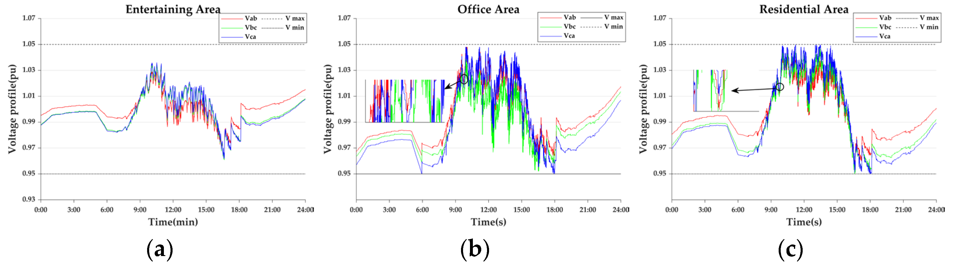
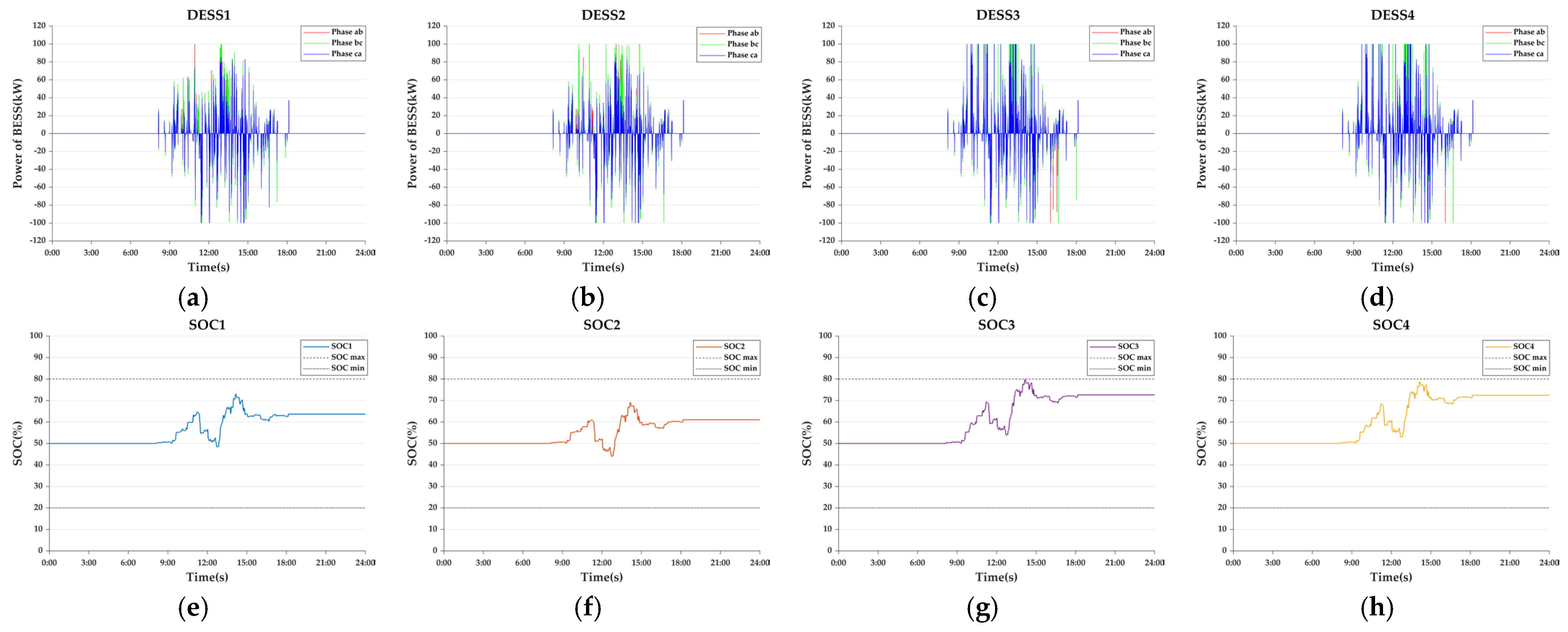
  • Case 2-5: Adaptive real-time control
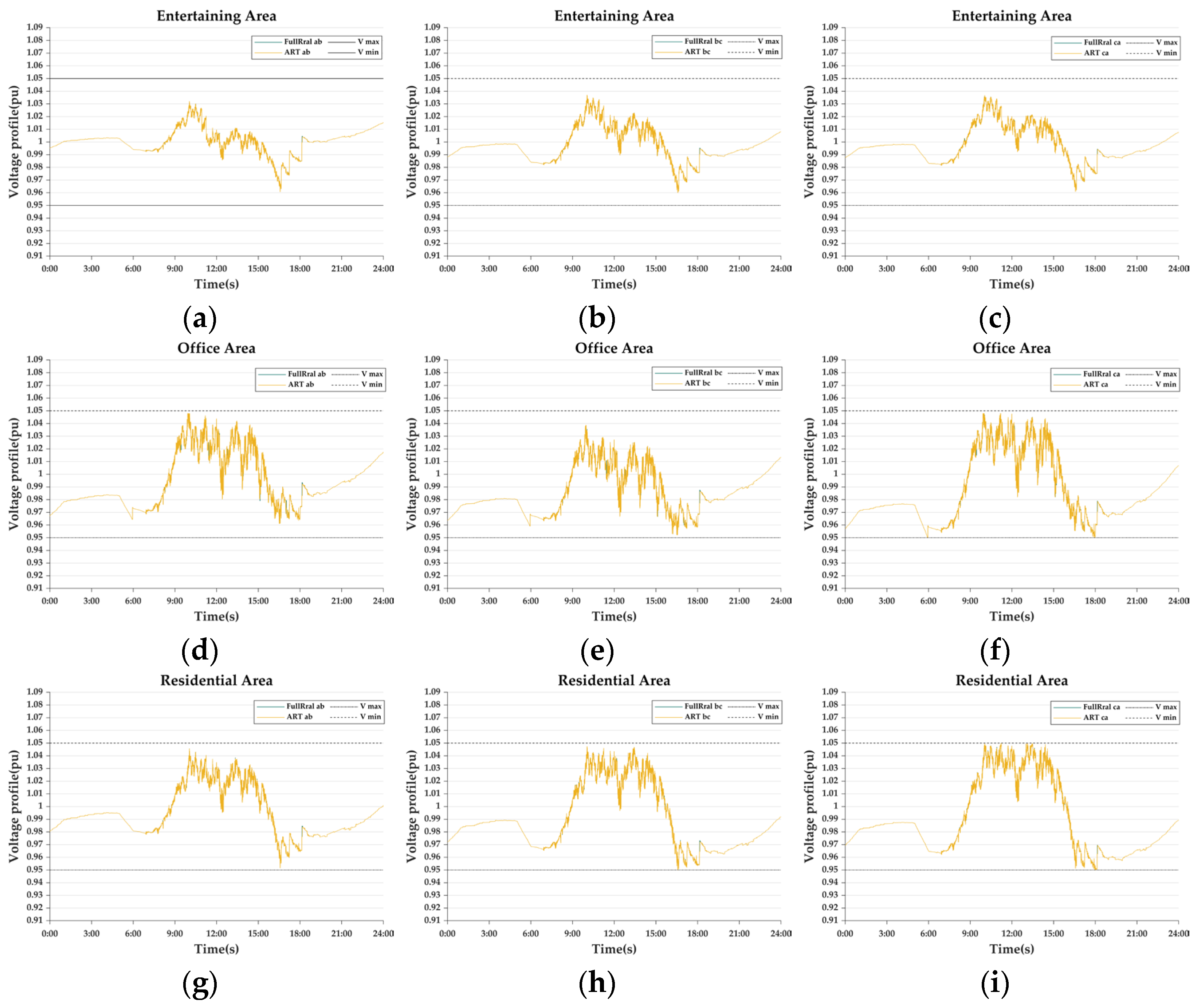
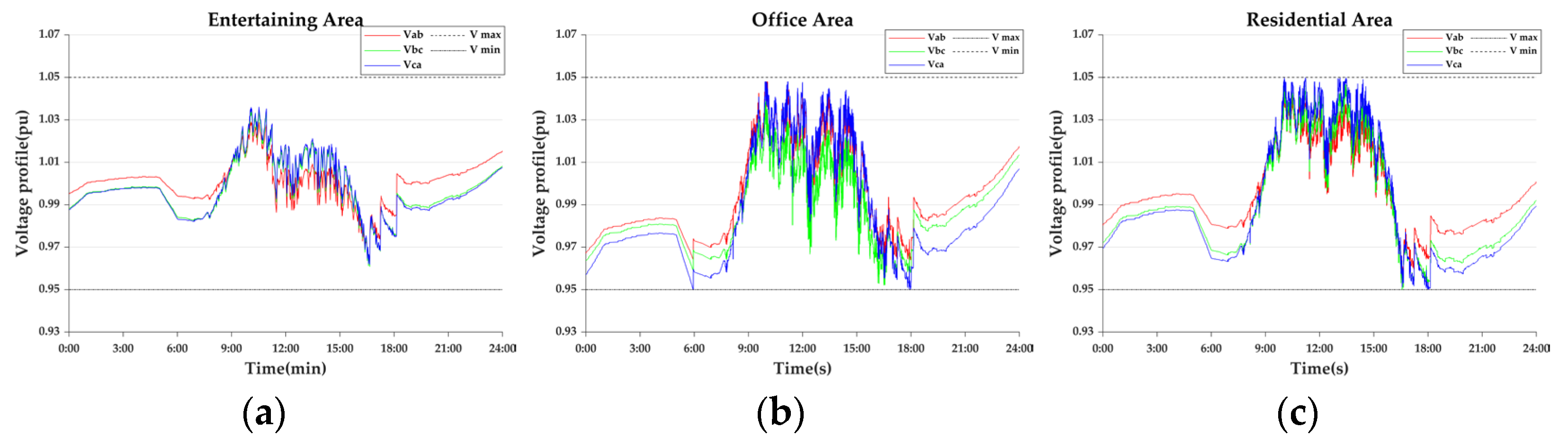
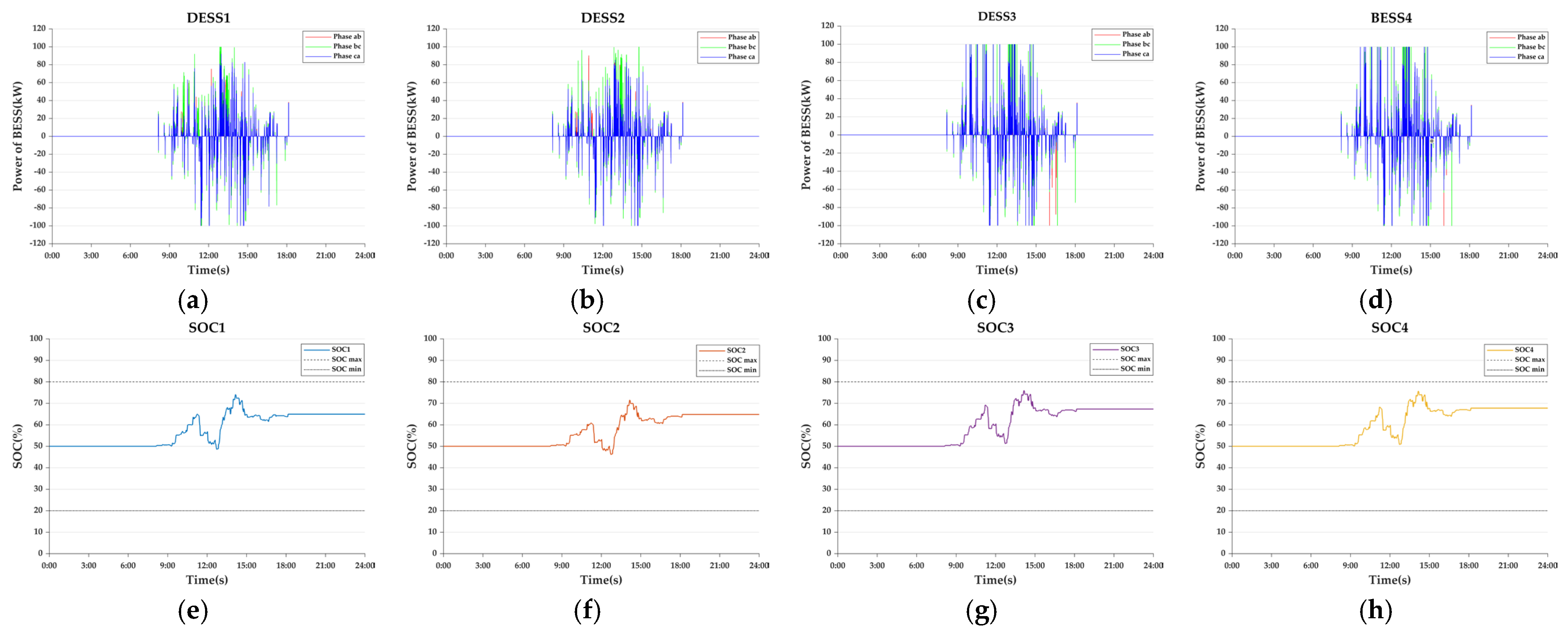
As is shown in Figure 16, real-time control can cope with the deterioration of voltage quality caused by the ultra-short-term fluctuations of PV output. However, continuous real-time control of all functional areas will bring a heavy sampling workload. As shown in Figure 16, when there is PV output that is extremely low, the voltage curve is relatively stable. To reduce the sampling workload, VQRPC proposed in this paper is used to determine the real-time control period of each functional area, as shown in Figure 18.
From Figure 18, the voltage in the entertainment area is stable and minute level control is used throughout the day. The residential and office areas use real-time control at times and minute-level control at times due to the differences in the distribution of EVs charging in the functional areas and the effect of coordinated control of SVR and OLTC. The sampling effort in entertainment area is only 16.7% of the real-time control, compared to 47.03% and 32.8% in the office and residential areas, respectively. A comparison of the three functional areas into real-time control periods is shown in Figure 19.
The voltage profile of each functional area under adaptive timescale control is shown in Figure 20.
From Figure 20, each functional area switches between minute-level optimisation and real-time control based on the real-time voltage status. A comparison of the voltage profile of each functional area under this strategy with the voltage profile after real-time control using the real-time adaptive control strategy is given in Appendix C.
From Figure 20, after the adaptive real-time control strategy is applied in real-time control, the voltage of each functional area remains within the safety threshold throughout the day. The sampling workloads required for entertainment area, office area, and residential area are 16.7%, 47.03%, and 32.8% respectively of that in the case of real-time control alone, and the voltage regulation effect is basically the same as that of real-time control. This verifies that the proposed adaptive real-time control can both improve power quality and reduce the sampling effort of real-time data in DN. The voltage fluctuation rate χ z , vf of each functional area under the three strategies of minute-level optimisation, adaptive real-time control and real-time control only is shown in Table 7.
The DESS output and SOC variations in each functional area under adaptive real-time control, as shown in Figure 21.
  • Case 2-6: DOM
In Case 2-5, the proposed adaptive real-time control strategy is adopted to significantly reduce the real-time data sampling workload of the DN. However, as seen in Figure 21g,h, the SOC of DESS3 and DESS4 in the office area reaches up to 79.83% and 78.82%, and deep charging occurs. In order to alleviate the deep charging/discharging problem of DESS, this paper proposes a deviation optimisation management strategy. After the implementation of this strategy, the voltage, DESS output and SOC variations in each functional area are shown in Figure 22 and Figure 23.
As shown in Figure 23, compared with Cases 2-5, the DOM strategy reduces the maximum SOC of DESS3 in the office area from 79.83% to 75.98%, with an increase of 6.42% in the available capacity; and reduces the maximum SOC of DESS4 from 78.82% to 75.71%, with an increase of 5.18% in the available capacity. The simulation results verify that the DMO strategy can improve the negative impact of deep charging and discharging on the cycle life of the DESS while at the same time improve the voltage quality and optimize the available capacity of the DESS. After applying the DMO strategy to the real-time control, the voltage profiles of each functional area are shown in Figure 24.
From Figure 24, the voltage in each functional areas is maintained within the safety thresholds throughout the day. Compared with Case 2-3, the suppresses voltage fluctuation in each functional area are significantly suppressed with 3.97% for χ z , vf in entertainment area, 11.72% for χ z , vf in office areas and 9.10% for χ z , vf in residential area. Although the voltage suppression effect of each functional areas is slightly weaker than that of Cases 2-4, it effectively improves the usable capacity of the DESS.
  • Case 2-7: EV, DESS Coordination Control
In this paper, EVs in functional areas are used to coordinate DESS output to alleviate the pressure on DESS capacity allocation. The voltage, DESS output, SOC variation, and EVs charging and discharging power profiles in each functional area after EVs coordinate DESS output are shown in Figure 25, Figure 26 and Figure 27.
As shown in Figure 25, compared with Cases 2-6, after the EVs are used to coordinate the DESS output, the output and output duration of the DESS in each functional area are reduced. The maximum SOCs of DESS1 and DESS2 in the residential area are reduced to 66.17% and 61.61%, respectively; and the maximum SOCs of DESS3 and DESS4 in the office area are reduced to 65.53% and 68.65%, respectively. According to Equation (71), the capacity reduction χ b , cur of DESS1, DESS2, DESS3 and DESS4 are 25.15%, 33.61%, 29.91% and 20.81%, respectively.
χ b , cur = Δ SOC b , bef Δ SOC b , lat Δ SOC b , bef
where Δ SOC b , bef is the capacity used by the bth DESS before EVs are coordinated. Δ SOC b , lat is the capacity used by the bth DESS after EVs coordination.
Figure 27 shows the coordinated output of EVs in each functional zone. In particular, the EVs in the entertainment area were not output due to the minute optimised control applied throughout the day. After the coordinated control of EV and DESS was applied to the real-time control, the voltage profile of each functional area is shown in Figure 28.

5. Conclusions

As the penetration of PVs and EVs in the DN continues to rise, strong random perturbations on both sides of the source-load can cause problems such as voltage violations and voltage fluctuations in the DN, This paper aims at the new DN field with high penetration rate of distributed photovoltaic power generation, and proposes a spatio-temporal adaptive voltage coordinated control strategy, complex scheduling through simple control techniques. The proposed strategy innovatively constructs a control system with regional division, multiple time scales, and multi-device synergy, and coordinates the control of OLTC, SVR, DESS, and EVs in different time scales and functional areas to realize the real-time improvement of voltage quality, and to reduce the workload of real-time data sampling while giving full effect to the voltage regulation capability of OLTC, SVR, and promoting the use of BESS and EVs. While real-time data sampling workload is reduced, OLTC, SVR voltage regulation capability is fully utilized, and the use of BESS and EVs is promoted, and the main conclusions are as follows:
Aiming at the frequent voltage fluctuations caused by the strong stochasticity of PV, a VMTB control strategy based on the DESS of functional areas is proposed to effectively suppress the voltage fluctuations, and the results of the study show that the voltage fluctuation rates of the entertainment area, the office area, and the residential area have been reduced by 29.21%, 40.53%, and 39.75%, respectively.
Aiming at the pressure on computation and storage etc. caused by continuous sampling of real-time data by the nodes of the whole network, a dynamic sensing mechanism of VQRPC based on partitioning decision is proposed. The results show that compared with the continuous real-time control in the whole area, the data collection workloads in entertainment, office and residential areas are reduced by 83.3%, 52.97% and 67.2%, respectively, while maintaining better voltage quality.
Aiming at SOC management, DOM strategy is introduced in VMTB, and the research results show that the maximum SOC of DESS3 in the workspace decreases by 3.85% and the available capacity is improved by 6.42%. The maximum SOC of BESS4 decreases by 3.11% and the available capacity is improved by 5.18%. It also proposes a management mechanism based on the available capacity of functional area DESS to further enhance SOC management and improve SOC homogenization. The study results show that the maximum SOC deviation of DESS in office area is only 1.17%, and the maximum SOC deviation of DESS in residential area is only 4.82%. In addition, in order to alleviate the pressure of DESS capacity allocation, EVs were used to coordinate the DESS output, and the results showed that the DESS3 and DESS3 capacities in the office area could be cut by 15.7% and 18.6%, respectively, and the DESS3 and DESS3 capacities in the residential area could be cut by 16.4% and 17.5%, respectively.
With the increase of PV penetration and EVs ownership in the distribution network, it intensifies the difficulty of voltage control in the DN in the future. Therefore, there is still a need for in-depth work in this study. In order to more fully validate the effectiveness of the proposed strategy, the applicability validation of large-scale real DN projects needs to be further promoted. Secondly, the reasonable selection of optimization algorithms plays a decisive role in improving the effect of real-time voltage control in DN. Therefore, screening the optimization algorithms suitable for voltage control of DN will help to realize more efficient and accurate real-time voltage control. In addition, in-depth analysis of the constraints faced by DESS during its application to real DN. This helps to optimize the energy distribution of DESS in DN, achieve accurate voltage control, and improve the efficiency and stability of system operation. Together, these aspects constitute our current research direction.

Author Contributions

Conceptualization, X.C. and X.Z.; methodology, X.C.; software, X.C. and Q.Y.; validation, X.C., X.Z. and Q.Y.; formal analysis, X.C. and Q.Y.; investigation, X.C. and X.Z.; data curation, Y.L.; writing—original draft preparation, X.C. and X.Z.; writing—review and editing, X.C. and Q.Y.; supervision, X.C. All authors have read and agreed to the published version of the manuscript.

Funding

This research was funded by The Key Science and Technology Program of Henan Province grant number [No. 252102240060].

Data Availability Statement

The data presented in this study are available on request from the corresponding author due to privacy.

Conflicts of Interest

Author Yanxue Li was employed by the company State Grid Integrated Energy Planning and D&R Institute Co., Ltd. The remaining authors declare that the research was conducted in the absence of any commercial or financial relationships that could be construed as a potential conflict of interest.

Appendix A

The specific implementation steps for the advance OLTC and SVR scheduling Program are as follows:
Step 1: Obtain the forecasting value of PV output through the AHA-LSSVM model and then substitute it into the power flow calculation to obtain the voltage of each node.
Step 2: When voltage satisfies Equation (A1), the tap positions of OLTC and SVR remain unchanged. Otherwise, calculate the voltage Δ V z t to be regulated for each functional area at time t according to Equation (A2).
V   min V z - i , da   n t     V   max
  Δ V z t = V z - i , da max t V   max   i f   V z - i , da max t > V   max V z - i , da min t V   min   i f   V z - i , da min t < V   min
V z - i , da max t =   max V z - i , da   n t
V z - i , da min t =   min V z - i , da   n t
where V z - i , da   n t is the voltage of phase n of node i in functional area z at time t during day-ahead scheduling. V z - i , da max t and V z - i , da min t are the maximum and minimum values of the voltage in functional area z at time t during day-ahead scheduling. V   max   and   V   min are upper and lower limits of voltage, respectively.
Step 3: Calculate the number R ( t ) of functional areas with voltage violations according to Equation (16). When R ( t )   >   1 , go to step 4 and use the OLTC for global voltage regulation. If not, go to step 5 and use the SVR for local voltage regulation.
R ( t )   = z = 1 Z R z ( t )
  R z ( t ) = 1   i f   V z - i , da   n t > V   max   o r   V z - i , da   n t < V   min 0   i f   V   min V z - i , da   n t V   max
where Z is the number of functional areas.
Step 4: Calculate the required operating tap position Δ N tap oltc t of OLTC at time t according to Equation (A7), and calculate the voltage V z - i reg t after OLTC operation according to Equation (A9):
Δ N tap oltc t = V tap oltc t Δ v tap oltc   i f   V tap oltc t > 0 V tap oltc t Δ v tap oltc   i f   V tap oltc t < 0
V tap oltc t = m a x Δ V z t   if   V z - i , da max t > V   max m i n Δ V z t   i f   V z - i , da min t < V   min
V z - i   reg t = V z - i , da   n t + Δ N tap oltc t · Δ v tap oltc
where V tap oltc t is the voltage that OLTC needs to regulate at time t. x is rounded up and x is rounded down.
When V z - i   reg t satisfies Equation (A1), the day-ahead scheduling voltage regulation process at time t is completed. Otherwise, proceed to Step 5 and implement the coordinated voltage regulation by SVR.
Step 5: Calculate the voltage Δ V tap   svr t that SVR needs to regulate according to Equation (21), and calculate the tap position Δ N tap svr t   that SVR needs to operate at time t according to Equation (A11):
Δ V tap   svr t = m a x Δ V z t + Δ N tap oltc t · Δ v tap oltc   if   V z - i , da m ax t > V   max m i n Δ V z t + Δ N tap oltc t · Δ v tap oltc   i f   V z - i , da m in t < V   SOC
Δ N tap svr t = V tap svr t Δ v tap svr   i f   V tap svr t > 0 V tap svr t Δ v tap svr   i f   V tap svr t < 0

Appendix B

A comparison of the voltage profiles before and after real-time control of each functional area is shown in Figure A1.
Figure A1. Real-time control of the voltage profile before and after. (a) voltage profile in phase ab of office areas; (b) voltage profile in phase bc of office areas; (c) voltage profile in phase ca of office areas; (d) voltage profile in phase ab of residential areas; (e) voltage profile in phase bc of residential areas; (f) voltage profile in phase ca of residential areas.
Energies 18 02093 g0a1

Appendix C

Figure A2. Comparison of real-time adaptive control and real-time control voltage profiles. (a) voltage profile in phase ab of entertainment area; (b) voltage profile in phase bc of entertainment area; (c) voltage profile in phase ca of entertainment area; (d) voltage profile in phase ab of office areas; (e) voltage profile in phase bc of office areas; (f) voltage profile in phase ca of office areas; (g) voltage profile in phase ab of residential areas; (h) voltage profile in phase bc of residential areas; (i) voltage profile in phase ca of residential areas.
Energies 18 02093 g0a2

References

  1. Wang, X.; Wang, G.; Chen, T.; Zeng, Z.; Heng, C.K. Low-Carbon City and Its Future Research Trends: A Bibliometric Analysis and Systematic Review. Sustain. Cities Soc. 2023, 90, 104381. [Google Scholar] [CrossRef]
  2. Zhang, Y.; Cao, Y.; Chen, T.; Lucchi, E. Optimized Community-Level Distributed Photovoltaic Generation (DPVG): Aesthetic, Technical, Economic, and Environmental Assessment of Building Integrated Photovoltaic (BIPV) Systems. J. Build. Eng. 2025, 103, 112085. [Google Scholar] [CrossRef]
  3. Ufa, R.A.; Malkova, Y.Y.; Rudnik, V.E.; Andreev, M.V.; Borisov, V.A. A Review on Distributed Generation Impacts on Electric Power System. Int. J. Hydrog. Energy 2022, 47, 20347–20361. [Google Scholar] [CrossRef]
  4. Yang, Z.; Yang, F.; Min, H.; Tian, H.; Hu, W.; Liu, J. Review on Optimal Planning of New Power Systems with Distributed Generations and Electric Vehicles. Energy Rep. 2023, 9, 501–509. [Google Scholar] [CrossRef]
  5. Kharrazi, A.; Sreeram, V.; Mishra, Y. Assessment Techniques of the Impact of Grid-Tied Rooftop Photovoltaic Generation on the Power Quality of Low Voltage Distribution Network—A Review. Renew. Sustain. Energy Rev. 2020, 120, 109643. [Google Scholar] [CrossRef]
  6. Ma, Y.; Huang, Y.; Yuan, Y. The Short-Term Forecasting of Distributed Photovoltaic Power Considering the Sensitivity of Meteorological Data. J. Clean. Prod. 2025, 486, 144599. [Google Scholar] [CrossRef]
  7. Kang, W.; Guan, Y.; Wang, H.; Vasquez, J.C.; Agundis-Tinajero, G.D.; Guerrero, J.M. Distributed Control of Virtual Energy Storage Systems for Voltage Regulation in Low Voltage Distribution Networks Subjects to Varying Time Delays. Appl. Energy 2024, 376, 124295. [Google Scholar] [CrossRef]
  8. Emrani-Rahaghi, P.; Hashemi-Dezaki, H.; Ketabi, A. Efficient Voltage Control of Low Voltage Distribution Networks Using Integrated Optimized Energy Management of Networked Residential Multi-Energy Microgrids. Appl. Energy 2023, 349, 121391. [Google Scholar] [CrossRef]
  9. Wang, Z.; Liu, H.; Wu, S.; Liu, N.; Liu, X.; Hu, Y.; Fu, Y. Explainable Time-Varying Directional Representations for Photovoltaic Power Generation Forecasting. J. Clean. Prod. 2024, 468, 143056. [Google Scholar] [CrossRef]
  10. Yuan, L.; Wang, X.; Sun, Y.; Liu, X.; Dong, Z.Y. Multistep Photovoltaic Power Forecasting Based on Multi-Timescale Fluctuation Aggregation Attention Mechanism and Contrastive Learning. Int. J. Electr. Power Energy Syst. 2025, 164, 110389. [Google Scholar] [CrossRef]
  11. Mahmoud, K.; Lehtonen, M. Three-Level Control Strategy for Minimizing Voltage Deviation and Flicker in PV-Rich Distribution Systems. Int. J. Electr. Power Energy Syst. 2020, 120, 105997. [Google Scholar] [CrossRef]
  12. Ferdowsi, F.; Mehraeen, S.; Upton, G.B. Assessing Distribution Network Sensitivity to Voltage Rise and Flicker under High Penetration of Behind-the-Meter Solar. Renew. Energy 2020, 152, 1227–1240. [Google Scholar] [CrossRef]
  13. Yu, P.; Zhang, H.; Hu, Z.; Song, Y. Voltage Control of Distribution Grid with District Cooling Systems Based on Scenario-Classified Reinforcement Learning. Appl. Energy 2025, 377, 124415. [Google Scholar] [CrossRef]
  14. Zhang, Z.; Li, P.; Ji, H.; Zhao, J.; Xi, W.; Wu, J.; Wang, C. Combined Central-Local Voltage Control of Inverter-Based DG in Active Distribution Networks1. Appl. Energy 2024, 372, 123813. [Google Scholar] [CrossRef]
  15. Song, G.; Wu, Q.; Jiao, W.; Lu, L. Distributed Coordinated Control for Voltage Regulation in Active Distribution Networks Based on Robust Model Predictive Control. Int. J. Electr. Power Energy Syst. 2025, 166, 110529. [Google Scholar] [CrossRef]
  16. Chen, Y.; Liu, Y.; Zhao, J.; Qiu, G.; Yin, H.; Li, Z. Physical-Assisted Multi-Agent Graph Reinforcement Learning Enabled Fast Voltage Regulation for PV-Rich Active Distribution Network. Appl. Energy 2023, 351, 121743. [Google Scholar] [CrossRef]
  17. Zhang, Z.; da Silva, F.F.; Guo, Y.; Bak, C.L.; Chen, Z. Double-Layer Stochastic Model Predictive Voltage Control in Active Distribution Networks with High Penetration of Renewables. Appl. Energy 2021, 302, 117530. [Google Scholar] [CrossRef]
  18. Ahmad, A.B.; Ooi, C.A.; Ali, O.; Charin, C.; Maharum, S.M.M.; Swadi, M.; Salem, M. Renewable Integration and Energy Storage Management and Conversion in Grid Systems: A Comprehensive Review. Energy Rep. 2025, 13, 2583–2602. [Google Scholar] [CrossRef]
  19. Li, S.; Liu, B.; Li, X. A Robust and Optimal Voltage Control Strategy for Low-Voltage Grids Utilizing Group Coordination of Photovoltaic and Energy Storage Systems via Consensus Algorithm. Int. J. Hydrog. Energy 2024, 78, 1332–1343. [Google Scholar] [CrossRef]
  20. Abdalla, A.N.; Nazir, M.S.; Tao, H.; Cao, S.; Ji, R.; Jiang, M.; Yao, L. Integration of Energy Storage System and Renewable Energy Sources Based on Artificial Intelligence: An Overview. J. Energy Storage 2021, 40, 102811. [Google Scholar] [CrossRef]
  21. Ali, M.U.; Zafar, A.; Nengroo, S.H.; Hussain, S.; Junaid Alvi, M.; Kim, H.-J. Towards a Smarter Battery Management System for Electric Vehicle Applications: A Critical Review of Lithium-Ion Battery State of Charge Estimation. Energies 2019, 12, 446. [Google Scholar] [CrossRef]
  22. González, I.; Calderón, A.J.; Folgado, F.J. IoT Real Time System for Monitoring Lithium-Ion Battery Long-Term Operation in Microgrids. J. Energy Storage 2022, 51, 104596. [Google Scholar] [CrossRef]
  23. Tao, Z.; Zhao, Z.; Wang, C.; Huang, L.; Jie, H.; Li, H.; Hao, Q.; Zhou, Y.; See, K.Y. State of Charge Estimation of Lithium Batteries: Review for Equivalent Circuit Model Methods. Measurement 2024, 236, 115148. [Google Scholar] [CrossRef]
  24. Wang, H.; Ye, Y.; Wang, Q.; Tang, Y.; Strbac, G. An Efficient LP-Based Approach for Spatial-Temporal Coordination of Electric Vehicles in Electricity-Transportation Nexus. IEEE Trans. Power Syst. 2023, 38, 2914–2925. [Google Scholar] [CrossRef]
  25. Fan, P.; Yang, J.; Ke, S.; Wen, Y.; Liu, X.; Ding, L.; Ullah, T. A Multilayer Voltage Intelligent Control Strategy for Distribution Networks with V2G and Power Energy Production-Consumption Units. Int. J. Electr. Power Energy Syst. 2024, 159, 110055. [Google Scholar] [CrossRef]
  26. Qian, J.; Jiang, Y.; Liu, X.; Wang, Q.; Wang, T.; Shi, Y.; Chen, W. Federated Reinforcement Learning for Electric Vehicles Charging Control on Distribution Networks. IEEE Inter. Things J. 2024, 11, 5511–5525. [Google Scholar] [CrossRef]
  27. Çelik, D.; Khan, M.A.; Khosravi, N.; Waseem, M.; Ahmed, H. A Review of Energy Storage Systems for Facilitating Large-Scale EV Charger Integration in Electric Power Grid. J. Energy Storage 2025, 112, 115496. [Google Scholar] [CrossRef]
  28. Yu, H.; Niu, S.; Shang, Y.; Shao, Z.; Jia, Y.; Jian, L. Electric Vehicles Integration and Vehicle-to-Grid Operation in Active Distribution Grids: A Comprehensive Review on Power Architectures, Grid Connection Standards and Typical Applications. Renew. Sustain. Energy Rev. 2022, 168, 112812. [Google Scholar] [CrossRef]
  29. Qi, T.; Ye, C.; Zhao, Y.; Li, L.; Ding, Y. Deep Reinforcement Learning Based Charging Scheduling for Household Electric Vehicles in Active Distribution Network. J. Mod. Power Syst. Clean Energy 2023, 11, 1890–1901. [Google Scholar] [CrossRef]
  30. Liu, D.; Zeng, P.; Cui, S.; Song, C. Deep Reinforcement Learning for Charging Scheduling of Electric Vehicles Considering Distribution Network Voltage Stability. Sensors 2023, 23, 1618. [Google Scholar] [CrossRef]
  31. Xiao, Q.; Zhang, R.; Wang, Y.; Shi, P.; Wang, X.; Chen, B.; Fan, C.; Chen, G. A Deep Reinforcement Learning Based Charging and Discharging Scheduling Strategy for Electric Vehicles. Energy Rep. 2024, 12, 4854–4863. [Google Scholar] [CrossRef]
  32. Hu, D.; Ye, Z.; Gao, Y.; Ye, Z.; Peng, Y.; Yu, N. Multi-Agent Deep Reinforcement Learning for Voltage Control With Coordinated Active and Reactive Power Optimization. IEEE Trans. Smart Grid 2022, 13, 4873–4886. [Google Scholar] [CrossRef]
  33. Hu, R.; Wang, W.; Wu, X.; Chen, Z.; Jing, L.; Ma, W.; Zeng, G. Coordinated Active and Reactive Power Control for Distribution Networks with High Penetrations of Photovoltaic Systems. Sol. Energy 2022, 231, 809–827. [Google Scholar] [CrossRef]
  34. Emarati, M.; Barani, M.; Farahmand, H.; Aghaei, J.; del Granado, P.C. A Two-Level over-Voltage Control Strategy in Distribution Networks with High PV Penetration. Int. J. Electr. Power Energy Syst. 2021, 130, 106763. [Google Scholar] [CrossRef]
  35. Khan, H.A.; Zuhaib, M.; Rihan, M. Voltage Fluctuation Mitigation with Coordinated OLTC and Energy Storage Control in High PV Penetrating Distribution Network. Electr. Power Syst. Res. 2022, 208, 107924. [Google Scholar] [CrossRef]
  36. Guo, Y.; Wu, Q.; Gao, H.; Huang, S.; Zhou, B.; Li, C. Double-Time-Scale Coordinated Voltage Control in Active Distribution Networks Based on MPC. IEEE Trans. Sustain. Energy 2020, 11, 294–303. [Google Scholar] [CrossRef]
  37. Song, G.; Wu, Q.; Tan, J.; Jiao, W.; Chen, J. Stochastic MPC Based Double-Time-Scale Voltage Regulation for Unbalanced Distribution Networks with Distributed Generators. Int. J. Electr. Power Energy Syst. 2024, 155, 109687. [Google Scholar] [CrossRef]
  38. Yan, Q.; Chen, X.; Xing, L.; Guo, X.; Zhu, C. Multi-Timescale Voltage Regulation for Distribution Network with High Photovoltaic Penetration via Coordinated Control of Multiple Devices. Energies 2024, 17, 3830. [Google Scholar] [CrossRef]
  39. Wang, J.; Wang, W.; Hu, X.; Qiu, L.; Zang, H. Black-Winged Kite Algorithm: A Nature-Inspired Meta-Heuristic for Solving Benchmark Functions and Engineering Problems. Artif. Intell. Rev. 2024, 57, 98. [Google Scholar] [CrossRef]
  40. Li, G.; Cui, G.; Zhao, Y.; Sun, R.; Yuan, H.; Li, L. Mid-Infrared C2H6 Telemetry Sensor Using 3.34 Μm ICL Based on Optimized Light Receiving System and BKA-DELM Model. Opt. Lasers Eng. 2025, 186, 108799. [Google Scholar] [CrossRef]
  41. Zhang, S.; Fu, Z.; An, D.; Yi, H. Network Security Situation Assessment Based on BKA and Cross Dual-Channel. J. Supercomput. 2025, 81, 461. [Google Scholar] [CrossRef]
  42. Octaviano, M.E.F.; de Araujo, L.R.; Penido, D.R.R. Allocation of BESS and State of Charge Management in Unbalanced Distribution Networks Considering the State of Health. Electr. Power Syst. Res. 2025, 242, 111467. [Google Scholar] [CrossRef]
  43. Vaičys, J.; Gudžius, S.; Jonaitis, A.; Račkienė, R.; Blinov, A.; Peftitsis, D. A Case Study of Optimising Energy Storage Dispatch: Convex Optimisation Approach with Degradation Considerations. J. Energy Storage 2024, 97, 112941. [Google Scholar] [CrossRef]
  44. Luo, L.; He, P.; Zhou, S.; Lou, G.; Fang, B.; Wang, P. Optimal Scheduling Strategy of EVs Considering the Limitation of Battery State Switching Times. Energy Rep. 2022, 8, 918–927. [Google Scholar] [CrossRef]
  45. Wang, W.; Tang, A.; Wei, F.; Yang, H.; Xinran, L.; Peng, J. Electric Vehicle Charging Load Forecasting Considering Weather Impact. Appl. Energy 2025, 383, 125337. [Google Scholar] [CrossRef]
  46. Afshar, M.; Mohammadi, M.R.; Abedini, M. A Novel Spatial–Temporal Model for Charging Plug Hybrid Electrical Vehicles Based on Traffic-Flow Analysis and Monte Carlo Method. ISA Trans. 2021, 114, 263–276. [Google Scholar] [CrossRef]
  47. Habib, S.; Ahmad, F.; Gulzar, M.M.; Ahmed, E.M.; Bilal, M. Electric Vehicle Charging Infrastructure Planning Model with Energy Management Strategies Considering EV Parking Behavior. Energy 2025, 316, 134421. [Google Scholar] [CrossRef]
  48. White Paper on Charging Behavior of Electric Vehicle Users in China 2022. Available online: https://www.nea.gov.cn/2023-03/20/c_1310703965.htm (accessed on 20 February 2025).
Figure 1. Flowchart of day-ahead scheduling plan.
Energies 18 02093 g001
Figure 2. Flowchart of the intra-day optimization phase.
Energies 18 02093 g002
Figure 3. Flowchart of voltage regulation mode.
Energies 18 02093 g003
Figure 4. Flowchart of voltage fluctuation suppression.
Energies 18 02093 g004
Figure 5. Framework of spatio-temporal adaptive voltage coordinated control strategy.
Energies 18 02093 g005
Figure 6. Modified IEEE 33 system.
Energies 18 02093 g006
Figure 7. Power of EVs charged at charging stations in each functional area. (a) Entertainment areas; (b) office areas; (c) residential areas.
Energies 18 02093 g007
Figure 8. Power of EVs charged at charging stations in each functional area.
Energies 18 02093 g008
Figure 9. Voltage profile in Case 1-1. (a) entertainment area voltage profile; (b) office areas voltage profile; (c) residential areas voltage profile.
Energies 18 02093 g009
Figure 10. Voltage profile in Case 1-2. (a) entertainment area voltage profile; (b) office areas voltage profile; (c) residential areas voltage profile.
Energies 18 02093 g010
Figure 11. Operation of OLTC and SVR in Case 1-2.
Energies 18 02093 g011
Figure 12. Voltage profile in Case 2-1. (a) entertainment area voltage profile; (b) office areas voltage profile; (c) residential areas voltage profile.
Energies 18 02093 g012
Figure 13. Voltage profile in Case 2-2. (a) entertainment area voltage profile; (b) office areas voltage profile; (c) residential areas voltage profile.
Energies 18 02093 g013
Figure 14. Operation of OLTC and SVR in Case 2-2.
Energies 18 02093 g014
Figure 15. Voltage profile in Case 2-3. (a) entertainment area voltage profile; (b) office areas voltage profile; (c) residential areas voltage profile.
Energies 18 02093 g015
Figure 16. Voltage profile in Case 2-4. (a) entertainment area voltage profile; (b) office areas voltage profile; (c) residential areas voltage profile.
Energies 18 02093 g016
Figure 17. DESS output and SOC profile in Case 2-4. (a) DESS1 output; (b) DESS2 output; (c) DESS3 output; (d) DESS4 output; (e) SOC1 profile; (f) SOC2 profile; (g) SOC3 profile; (h) SOC4 profile.
Energies 18 02093 g017
Figure 18. Time period for each functional area to enter real-time control. (a) entertainment area; (b) office areas; (c) residential areas.
Energies 18 02093 g018
Figure 19. Three functional areas entered into real-time control for the period.
Energies 18 02093 g019
Figure 20. Voltage profile in Case 2-5. (a) entertainment area voltage profile; (b) office areas voltage profile; (c) residential areas voltage profile.
Energies 18 02093 g020
Figure 21. DESS output and SOC profile in Case 2-5. (a) DESS1 output; (b) DESS2 output; (c) DESS3 output; (d) DESS4 output; (e) SOC1 profile; (f) SOC2 profile; (g) SOC3 profile; (h) SOC4 profile.
Energies 18 02093 g021
Figure 22. Voltage profile in Case 2-6. (a) entertainment area voltage profile; (b) office areas voltage profile; (c) residential areas voltage profile.
Energies 18 02093 g022
Figure 23. DESS output and SOC profile in Case 2-6. (a) DESS1 output; (b) DESS2 output; (c) DESS3 output; (d) DESS4 output; (e) SOC1 profile; (f) SOC2 profile; (g) SOC3 profile; (h) SOC4 profile.
Energies 18 02093 g023
Figure 24. Full real-time voltage profile in Case 2-6. (a) entertainment area voltage profile; (b) office areas voltage profile; (c) residential areas voltage profile.
Energies 18 02093 g024
Figure 25. Voltage profile in Case 2-7. (a) entertainment area voltage profile; (b) office areas voltage profile; (c) residential areas voltage profile.
Energies 18 02093 g025
Figure 26. DESS output and SOC profile in Case 2-7. (a) DESS1 output; (b) DESS2 output; (c) DESS3 output; (d) DESS4 output; (e) SOC1 profile; (f) SOC2 profile; (g) SOC3 profile; (h) SOC4 profile.
Energies 18 02093 g026
Figure 27. EVs charging and discharging power by functional area. (a) entertainment area; (b) office areas; (c) residential areas.
Energies 18 02093 g027
Figure 28. Full real-time voltage profile in Case 2-7. (a) entertainment area voltage profile; (b) office areas voltage profile; (c) residential areas voltage profile.
Energies 18 02093 g028
Table 1. Parameters of distribution network.
ParameterValue
Voltage grade (kV)35
Total load (MW) 14.8
Total PV power (MW)15.6
Rated voltage (pu)1.0
Limit of node voltage (pu)[0.95, 1.05]
Day-ahead scheduling sample interval (min)5
Minute-level optimization sample interval (min)1
Real-time optimization control sample interval (s)10
Table 2. Parameters of voltage regulation equipment.
DeviceLocationParameterValue
DESS1
DESS2
DESS3
DESS4
Bus 33
Bus 31
Bus 18
Bus 16
Capacity (kWh)150
Power limit (kW)[−100, 100]
Charging/discharging efficiency (%) 100
SOC limit (%)[20, 80]
Initial SOC (%)50
EVCS1
EVCS2
EVCS3
Bus 17
Bus 30
Bus 4
Fast charging power (kW)60
Slow charging power (kW)7
Charging/discharging efficiency (%)90
OLTCHV Bus–MV Bus Tap range[−5, 5]
Per tap (%)2
SVRBus 7–Bus 8Tap range [−5, 5]
Per tap (%)1
Table 3. Parameters setting.
ParameterValue
sampling points ο 5
PV output start T st time (h)6:55
PV output end T ed time (h)18:40
Penalty value k pen 1000
Upper limit of deviation ψ max (%)0.3
Lower limit of deviation ψ min   (%)−0.3
PV output peak time T peak   (h)12:00
Expected   SOC ex , h before T peak   (%)0.6
Expected   SOC ex , l after T peak   (%)0.4
Weight α 1 0.55
Weight α 2 0.45
Constant k vfs 0.1
n tp 3
Table 4. Case study.
OLTCSVRDESSEV
Case 1: Day-ahead schedulingCase 1-1
Case 1-2
Case 2: Intra-day optimizationCase 2-1
Case 2-2
Case 2-3
Case 2-4VRFS
Case 2-5VRFS
Case 2-6VRFSDOM
Case 2-7VRFSDOM
✓: Involved.
Table 5. Functional areas T z , vvd and χ z , vf .
Entertaining AreaOffice AreaResidential Area
T z , vvd     % 01.832.46
χ z , vf     % 5.3419.2214.11
Table 6. Maximum and minimum SOC for each DESS.
DESS1DESS2DESS3DESS4
SOC max   % 72.8969.2679.8378.82
SOC min   % 48.4743.6850.0050.00
Table 7. χ z , vf under the three strategies.
Entertaining AreaOffice AreaResidential Area
Case 2-35.3419.2214.11
Case 2-43.7811.438.51
Case 2-53.8511.818.79
Disclaimer/Publisher’s Note: The statements, opinions and data contained in all publications are solely those of the individual author(s) and contributor(s) and not of MDPI and/or the editor(s). MDPI and/or the editor(s) disclaim responsibility for any injury to people or property resulting from any ideas, methods, instructions or products referred to in the content.

