
Robust Energy Management of Fuel Cell Hybrid Electric Vehicles Using Fuzzy Logic Integrated with H-Infinity Control


Abstract
1. Introduction
1.1. Literature Review
1.2. Motivation and Contribution
- Development of a hierarchical control framework that integrates fuzzy logic for intelligent power allocation with H-infinity control for robustness.
- Implementation of an energy management strategy that dynamically adjusts power distribution based on real-time system states and driving conditions.
- Evaluation of the proposed control framework under different vehicle configurations and drive cycles to validate its ability to enhance hydrogen efficiency, extend battery lifespan, and improve system robustness.
1.3. Organization of the Article
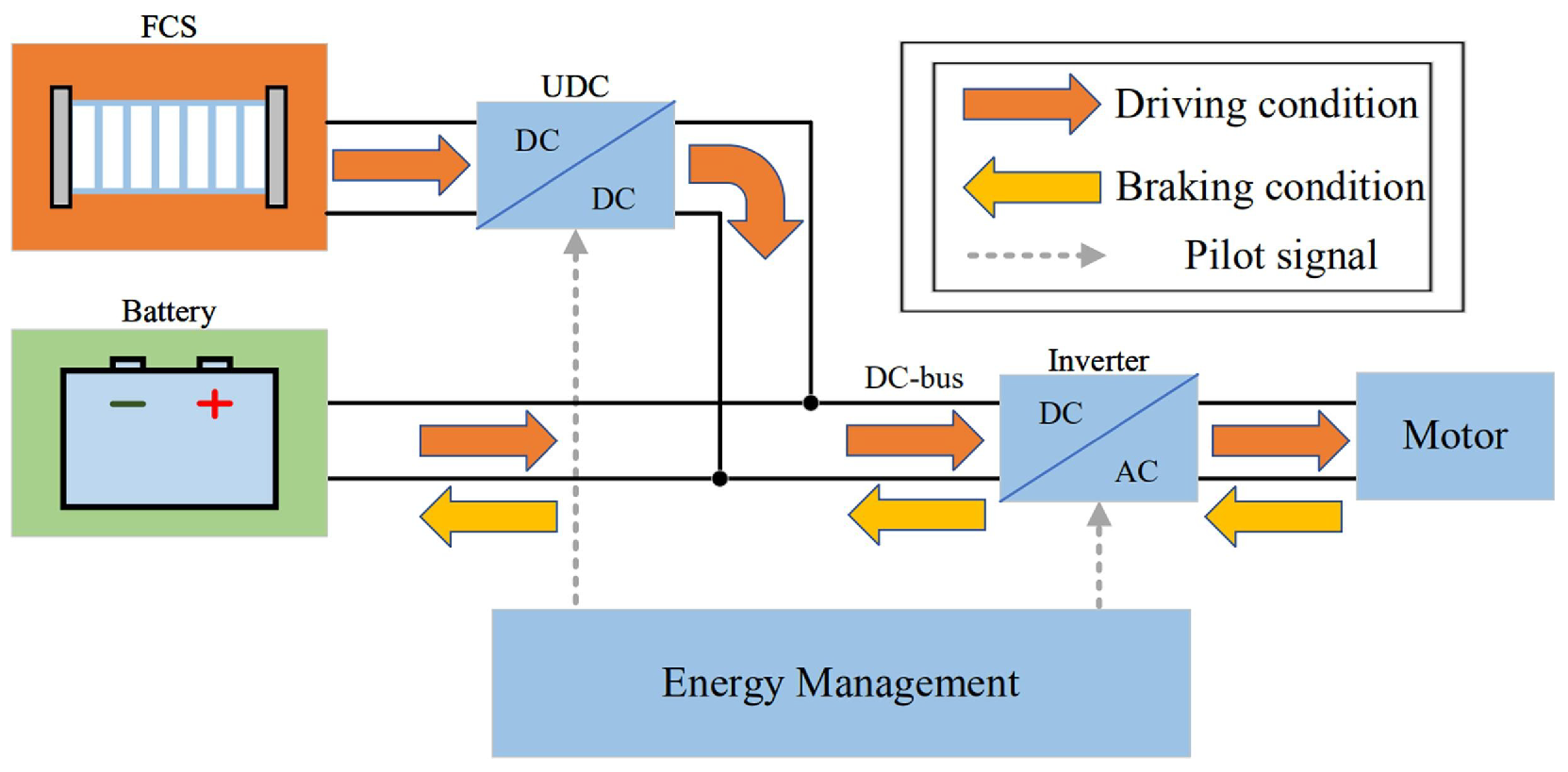
2. System Overview
- Fuel cell: A proton-exchange membrane fuel cell (PEMFC) that generates electrical power using hydrogen as fuel.
- Battery: Stores electrical energy and provides power during high demand or when the fuel cell is unavailable.
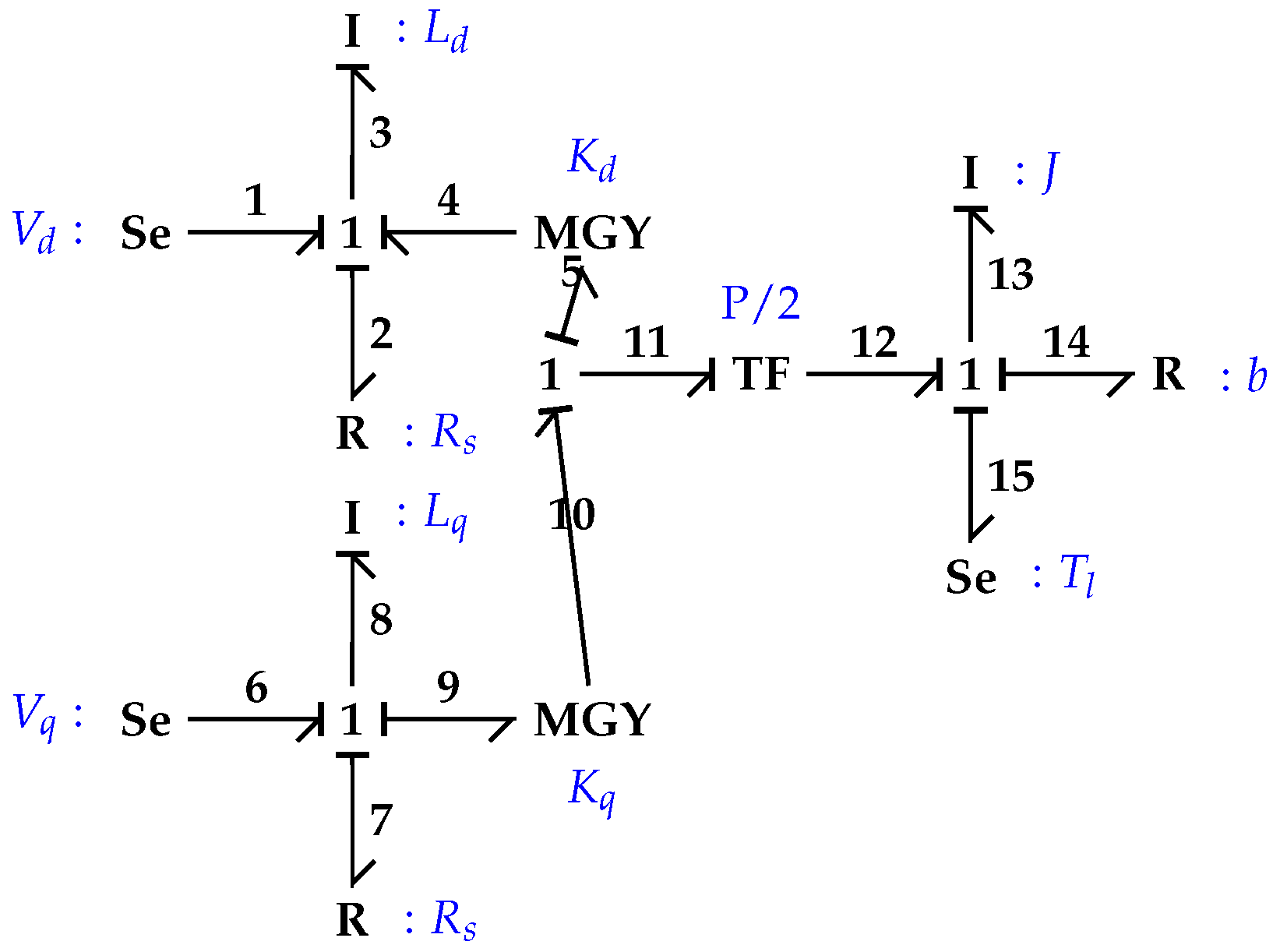
- Motor: A permanent magnet synchronous motor (PMSM) that drives wheels, ensuring high efficiency and torque control. A bond graph is implemented to find the dynamic equation of a PMSM [10].
- Vehicle model: The vehicle model of a rigid vehicle body with constant mass undergoing longitudinal motion.
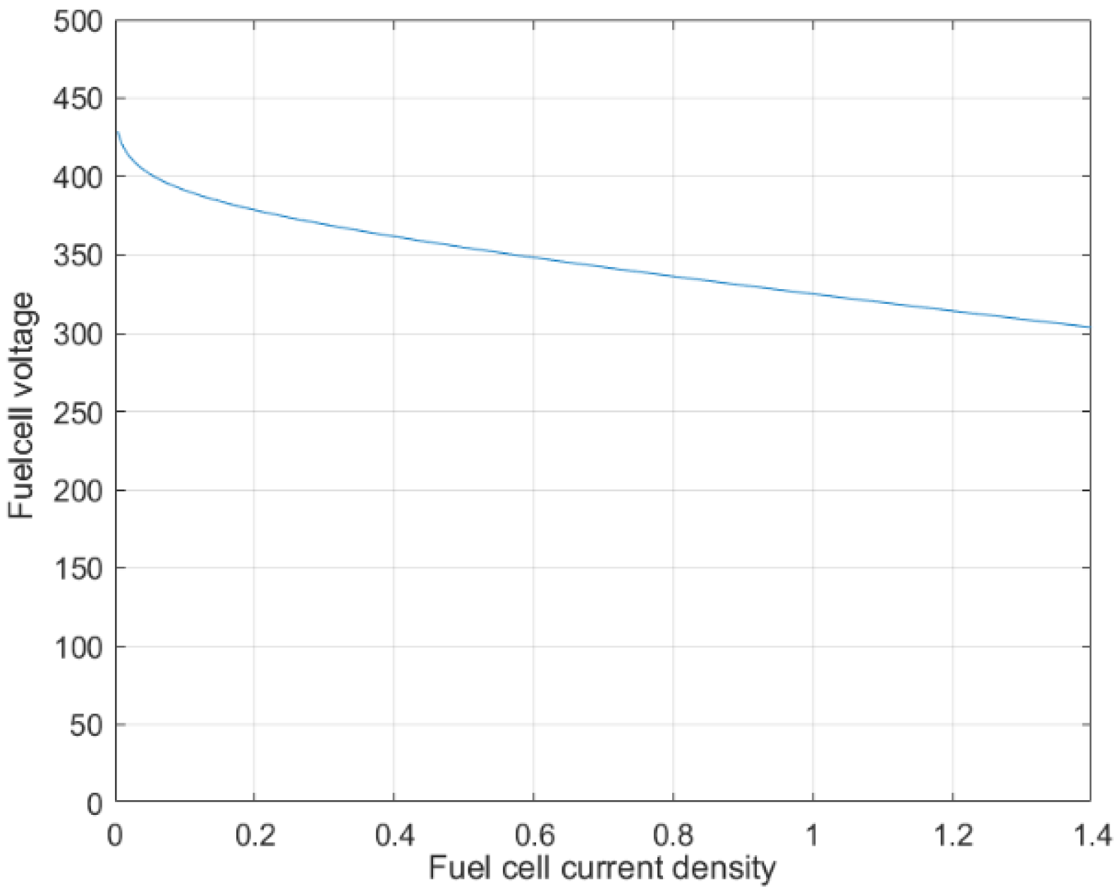
2.1. Fuel Cell
2.1.1. Open Circuit Voltage of the Fuel Cell
2.1.2. Irreversible Voltage Losses in the Fuel Cell
2.1.3. Activation Losses
2.1.4. Concentration Losses
2.1.5. Ohmic Losses
2.1.6. Reactant Flow Equations
2.1.7. Double-Layer Capacitance
2.1.8. State Space Model
2.2. Battery
- Series resistance:
- Battery open-circuit voltage:
- Resistance for the nth RC pair:
- Capacitance for the nth RC pair:
- is the terminal voltage of the battery.
- is the per-module battery current.
- represents the voltage drop across the n-th RC pair.
- The integration accounts for the transient response of the battery system.
- is the total battery capacity.
- The positive current () indicates battery discharge.
- The negative current () indicates battery charging.
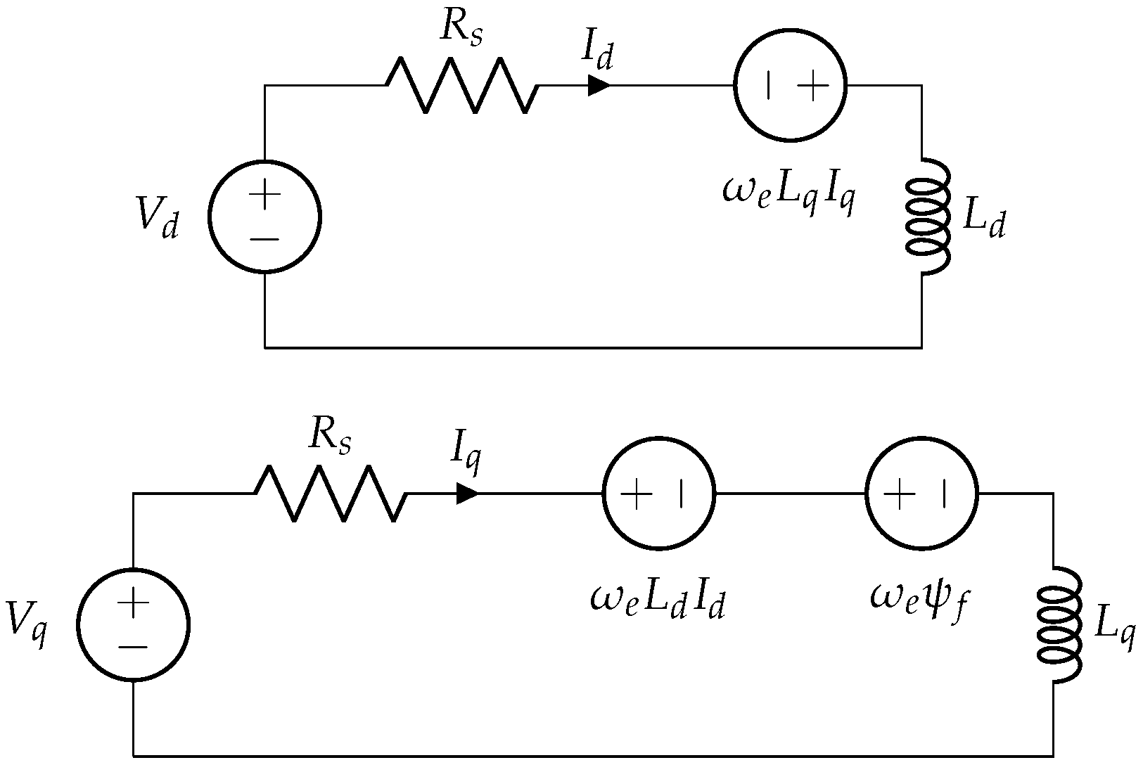
2.3. Motor
2.4. Vehicle Model
- is the total traction force required (N).
- m is the vehicle mass (kg).
- g is the acceleration due to gravity.
- is the rolling resistance coefficient, accounting for the friction between the tires and the road surface.
- is the road slope (degree), affecting the gravitational force component along the incline.
- is the aerodynamic drag coefficient, which quantifies the resistance due to airflow.
- A is the frontal windward area of the vehicle ().
- is the air density (kg/), influencing aerodynamic drag.
- V is the vehicle speed (m/s).
- a is the vehicle acceleration (m/).
- The first term, , accounts for rolling resistance, which is dependent on the vehicle weight and road-contact friction.
- The second term, , represents the aerodynamic drag, which increases with the velocity squared.
- The third term, , considers the gravitational force component acting along the inclined road.
- The last term, , denotes the inertial force, which is a function of the vehicle’s acceleration
- is the total power request (W).
- is the traction force (N).
3. Low-Level Controllers
3.1. Driver Controller
3.2. Motor Controller
3.3. Fuel Cell Controller
4. Ems/Higher-Level Controller
4.1. Mode Selector
- The driver’s power request ().
- The state of charge (SOC) of the battery.
4.2. Fuzzy Logic-Based EMS
4.2.1. Fuzzy Logic Structure
4.2.2. Fuzzy Rule Base and Decision Making
4.2.3. Defuzzification and Implementation
4.2.4. Power Transition Dynamics and Drive Conditions
4.2.5. Boundary Behavior and SOC Mode Switching
4.3. Robustness Against Model Uncertainty
4.3.1. Reference Generation and Motivation
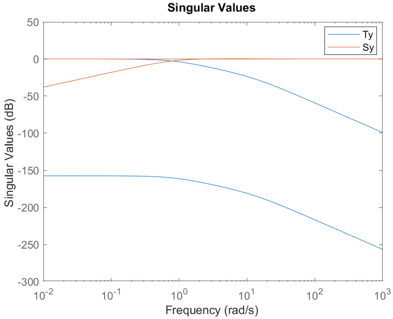
4.3.2. H-Infinity Control Architecture
4.3.3. H-Infinity Controller and Null Space Allocator Design
4.4. Interaction Between FLC and Controller
- FLC: Computes reference vector .
- controller: Tracks reference r by minimizing where , and .
- Plant: Receives from the controller and computes .
5. Results and Discussion
5.1. Fuzzy Logic Control Performance
5.2. Performance Analysis for UDDS Drive Cycle
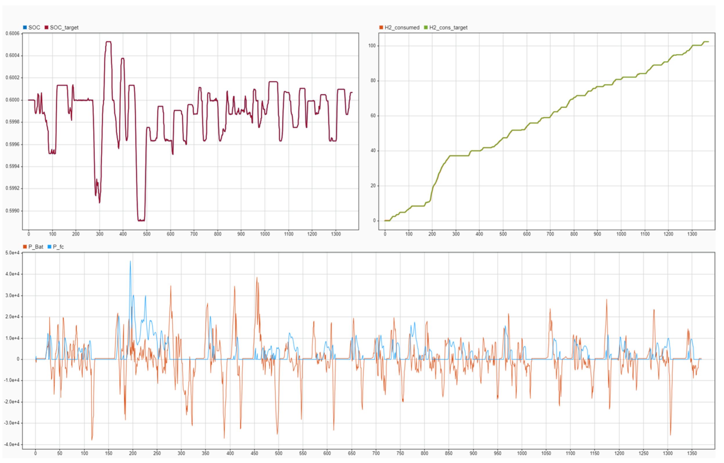
- Power split between and , showing how the controller allocates power between the fuel cell and battery during different driving conditions.
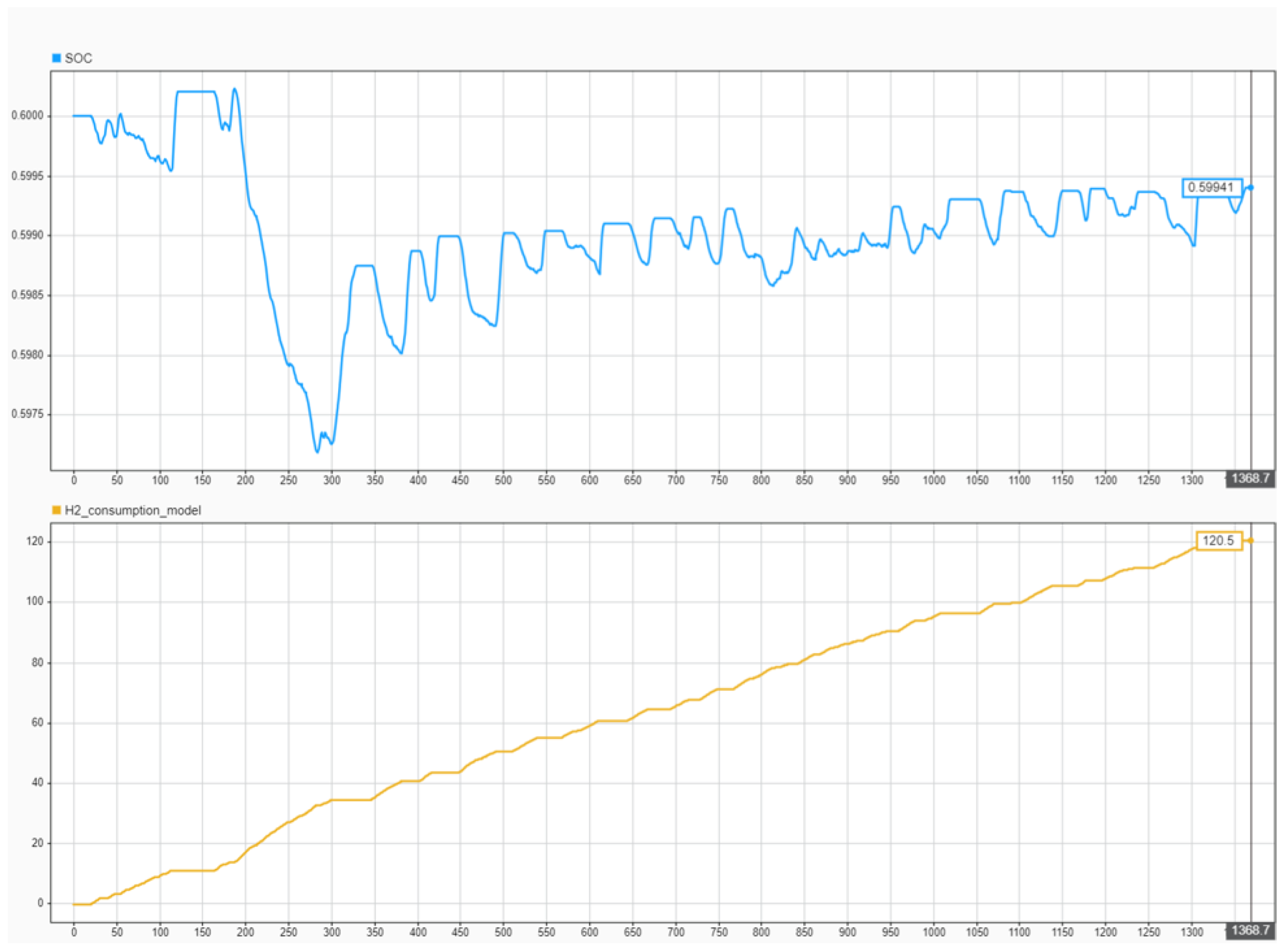
- SOC trajectory and hydrogen consumption trend, indicating whether the controller successfully regulates the SOC toward the target value while minimizing hydrogen usage.
5.3. Comparative Analysis: FLC vs. Dynamic Programming Benchmark
5.4. H-Infinity Controller and Performance
- Case 1: without Null-Space Allocator (Under-Actuated)
- Case 2: with Null-Space Allocator (Nominal Conditions)
- Case 3: with under Model Uncertainty
5.5. Discussion
6. Conclusions
Author Contributions
Funding
Data Availability Statement
Conflicts of Interest
References
- Djouahi, A.; Negrou, B.; Touggui, Y.; Samy, M. Optimal sizing and thermal control in a fuel cell hybrid electric vehicle via FC-HEV application. J. Braz. Soc. Mech. Sci. Eng. 2023, 45, 533. [Google Scholar] [CrossRef]
- Jensen, H.C.B.; Schaltz, E.; Koustrup, P.S.; Andreasen, S.J.; Kaer, S.K. Evaluation of Fuel-Cell Range Extender Impact on Hybrid Electrical Vehicle Performance. IEEE Trans. Veh. Technol. 2012, 62, 50–60. [Google Scholar] [CrossRef]
- Lachhab, I.; Krichen, L. An improved energy management strategy for FC/UC hybrid electric vehicles propelled by motor-wheels. Int. J. Hydrogen Energy 2014, 39, 571–581. [Google Scholar] [CrossRef]
- Zhou, J.; Du, P.; Liang, G.; Chang, H.; Liu, S. Hydrogen station location optimization coupling hydrogen sources and transportation along the expressway. Int. J. Hydrogen Energy 2024, 54, 1094–1109. [Google Scholar] [CrossRef]
- Silva, F.L.; Eckert, J.J.; Miranda, M.H.R.; da Silva, S.F.; Silva, L.C.A.; Dedini, F.G. A comparative analysis of optimized gear shifting controls for minimizing fuel consumption and engine emissions using neural networks, fuzzy logic, and rule-based approaches. Eng. Appl. Artif. Intell. 2024, 135, 108777. [Google Scholar] [CrossRef]
- Chen, J.; Wang, Q.; Su, B.; Shen, L.; Wang, Z. A Hybrid Power-Performance Adjustment Strategy for Clustered Multi-threading Architecture. In Proceedings of the 2016 IEEE 18th International Conference on High Performance Computing and Communications; IEEE 14th International Conference on Smart City; IEEE 2nd International Conference on Data Science and Systems (HPCC/SmartCity/DSS), Sydney, NSW, Australia, 12–14 December 2016; pp. 292–300. [Google Scholar] [CrossRef]
- Fletcher, T.; Thring, R.; Watkinson, M. An Energy Management Strategy to concurrently optimise fuel consumption & PEM fuel cell lifetime in a hybrid vehicle. Int. J. Hydrogen Energy 2016, 41, 21503–21515. [Google Scholar] [CrossRef]
- Gao, Z.; Wang, Y.; Ji, Z. Finite-time control of switched affine non-linear systems based on the Lie derivative and iteration technique. IET Control Theory Appl. 2019, 13, 3148–3154. [Google Scholar] [CrossRef]
- Glover, K.; Doyle, J.C. A state space approach to H∞ optimal control. In Three Decades of Mathematical System Theory: A Collection of Surveys at the Occasion of the 50th Birthday of Jan C. Willems; Nijmeijer, H., Schumacher, J.M., Eds.; Springer: Berlin/Heidelberg, Germany, 2005; pp. 179–218. [Google Scholar] [CrossRef]
- Karnopp, D.C.; Margolis, D.L.; Rosenberg, R.C. System Dynamics: Modeling, Simulation, and Control of Mechatronic Systems, 1st ed.; Wiley: Hoboken, NJ, USA, 2012. [Google Scholar] [CrossRef]
- Zhao, X.; Wang, L.; Zhou, Y.; Pan, B.; Wang, R.; Wang, L.; Yan, X. Energy management strategies for fuel cell hybrid electric vehicles: Classification, comparison, and outlook. Energy Convers. Manag. 2022, 270, 116179. [Google Scholar] [CrossRef]
- Larminie, J. Fuel Cell Systems Explained; Wiley: Hoboken, NJ, USA, 2003. [Google Scholar]
- Barać, B.; Krpan, M.; Capuder, T. Modelling of PEM Fuel Cell for Power System Dynamic Studies. IEEE Trans. Power Syst. 2023, 39, 3286–3298. [Google Scholar] [CrossRef]
- Ahmed, R.; Gazzarri, J.; Onori, S.; Habibi, S.; Jackey, R.; Rzemien, K.; Tjong, J.; Lesage, J. Model-Based Parameter Identification of Healthy and Aged Li-ion Batteries for Electric Vehicle Applications. Sae Int. J. Altern. Powertrains 2015, 4, 233–247. [Google Scholar] [CrossRef]
- Huria, T.; Ceraolo, M.; Gazzarri, J.; Jackey, R. High fidelity electrical model with thermal dependence for characterization and simulation of high power lithium battery cells. In Proceedings of the 2012 IEEE International Electric Vehicle Conference, Greenville, SC, USA, 4–8 March 2012; pp. 1–8. [Google Scholar] [CrossRef]
- Ba, X.; Gong, Z.; Guo, Y.; Zhang, C.; Zhu, J. Development of Equivalent Circuit Models of Permanent Magnet Synchronous Motors Considering Core Loss. Energies 2022, 15, 1995. [Google Scholar] [CrossRef]
- Parvathi, R.; Nisha, P. Modeling of Interior Permanent Magnet Synchronous Motor using Transient Simulation Techniques. Int. J. Innov. Sci. Eng. Technol. 2016, 3, 409–413. [Google Scholar]
- Lü, X.; Qian, S.; Zhai, X.; Wang, P.; Wu, T. Adaptive energy management strategy for FCHEV based on improved proximal policy optimization in deep reinforcement learning algorithm. Energy Convers. Manag. 2024, 321, 118977. [Google Scholar] [CrossRef]
- Zadeh, L.A. Fuzzy sets. Inf. Control 1965, 8, 338–353. [Google Scholar] [CrossRef]
- Filipozzi, L.; Assadian, F. Control of Over-Actuated Systems—From Practical to Theoretical Concepts with Application in Hybrid Powertrain Speed Control Development. In Proceedings of the 2022 IEEE Vehicle Power and Propulsion Conference (VPPC), Merced, CA, USA, 1–4 November 2022; pp. 1–6, ISSN 1938-8756. [Google Scholar] [CrossRef]
- Assadian, F.; Mallon, K.R. Robust Control: Youla Parameterization Approach; John Wiley & Sons: Hoboken, NJ, USA, 2022. [Google Scholar]


| Components | Parameters | Values |
|---|---|---|
| Vehicle | Mass | 2200 kg |
| Frontal area | 4 | |
| Air resistance coefficient | 0.3 | |
| Rolling radius | 0.35 m | |
| Rolling resistance coefficient | 0.013 | |
| Gravitational acceleration | 9.8 m/ | |
| Fuel cell | Maximum power | 106 kW |
| Efficiency | 0.55–0.6 | |
| No. of fuel cells | 436 | |
| Battery | Capacity | 102 Ah |
| Maximum discharge power | −78 kW | |
| Maximum charge power | 78 kW | |
| Motor | Maximum power | 300 kW |
| Maximum torque | 500 Nm | |
| Nominal speed | 5800 rpm | |
| Maximum speed | 21,000 rpm | |
| Efficiency | 1.00 |
| Mode | Power Request () | SOC Range (%) | Description |
|---|---|---|---|
| Regeneration Mode | Any | Regenerative braking mode where kinetic energy is converted to electrical energy and stored in the battery. | |
| Fuel Cell-Dominant Mode | 0–40 | Pure Fuel Cell Mode: The fuel cell solely meets the power request (). | |
| 0–40 | Hybrid Mode: The fuel cell operates at maximum power while the battery supplements the remaining demand (). | ||
| Hybrid Mode with SOC Regulation | Any | 40–70 | The system maintains SOC at a target level () by optimally splitting power between the fuel cell and battery using an FLC. |
| Battery Dominant Mode | Normal Conditions | 70–100 | Pure Battery Mode: The battery alone meets the power request (). |
| High-power request | 70–100 | Temporary Hybrid Mode: The battery provides maximum power while the fuel cell supplements additional demand (). |
| Driving Cycle | SOC Initial | Consumed [g] | SOC Final |
|---|---|---|---|
| UDDS | Pure FC | 165.3 | - |
| 40 | 120 | 40.66 | |
| 60 | 93 | 59.94 | |
| 70 | 85 | 69.60 | |
| US06 | Pure FC | 322.1 | - |
| 40 | 215.3 | 40.54 | |
| 60 | 152.2 | 59.01 | |
| 70 | 100.1 | 68.45 | |
| HWY | Pure FC | 177.9 | - |
| 40 | 141.9 | 40.18 | |
| 60 | 120.2 | 58.81 | |
| 70 | 110.8 | 68.42 | |
| NEDC | Pure FC | 166.5 | - |
| 40 | 128.1 | 40.34 | |
| 60 | 91.3 | 59.58 | |
| 70 | 85.4 | 69.28 | |
| WLTP | Pure FC | 362 | - |
| 40 | 238.1 | 40.40 | |
| 60 | 179.5 | 58.74 | |
| 70 | 151.2 | 67.98 |
| Drive Cycle | DP (g) | FLC (g) |
|---|---|---|
| UDDS | 56.00 | 93.00 |
| US06 | 122.75 | 152.24 |
| HWY | 102.40 | 120.20 |
| NEDC | 56.40 | 91.30 |
| WLTP | 156.40 | 179.5 |
Disclaimer/Publisher’s Note: The statements, opinions and data contained in all publications are solely those of the individual author(s) and contributor(s) and not of MDPI and/or the editor(s). MDPI and/or the editor(s) disclaim responsibility for any injury to people or property resulting from any ideas, methods, instructions or products referred to in the content. |
© 2025 by the authors. Licensee MDPI, Basel, Switzerland. This article is an open access article distributed under the terms and conditions of the Creative Commons Attribution (CC BY) license (https://creativecommons.org/licenses/by/4.0/).
Share and Cite
Yadav, S.; Assadian, F. Robust Energy Management of Fuel Cell Hybrid Electric Vehicles Using Fuzzy Logic Integrated with H-Infinity Control. Energies 2025, 18, 2107. https://doi.org/10.3390/en18082107
Yadav S, Assadian F. Robust Energy Management of Fuel Cell Hybrid Electric Vehicles Using Fuzzy Logic Integrated with H-Infinity Control. Energies. 2025; 18(8):2107. https://doi.org/10.3390/en18082107
Chicago/Turabian StyleYadav, Siddhesh, and Francis Assadian. 2025. "Robust Energy Management of Fuel Cell Hybrid Electric Vehicles Using Fuzzy Logic Integrated with H-Infinity Control" Energies 18, no. 8: 2107. https://doi.org/10.3390/en18082107
APA StyleYadav, S., & Assadian, F. (2025). Robust Energy Management of Fuel Cell Hybrid Electric Vehicles Using Fuzzy Logic Integrated with H-Infinity Control. Energies, 18(8), 2107. https://doi.org/10.3390/en18082107