Abstract
To fully utilize the reactive power resources of distributed photovoltaic (PV) systems, this study proposes a coordinated var-voltage control strategy for the main distribution network, incorporating the reactive power regulation capability of distributed PV. Firstly, the Automatic Voltage Control (AVC) tertiary and secondary voltage control methods and optimization models in the main and distribution networks area are analyzed, and the physical equivalence of the reactive power compensation equipment involved is carried out. In this study, a coordinated local var-voltage control method is proposed, which integrates AVC primary voltage control and divides the control scheme into feeder and station areas, respectively. Through the analysis of actual operation cases in a regional power grid, the results demonstrate a reduction in network loss by 171.14 kW through voltage adjustment, validating the effectiveness of the proposed strategy. This method fully leverages the reactive power regulation capability of distributed renewable energy sources, reduces the operational frequency of reactive power equipment in substations, and synergizes with the AVC system to achieve optimal power grid operation.
1. Introduction
With the rapid development of renewable energy, the proportion of distributed photovoltaic (PV) power generation on the load side is increasing year by year [1,2]. Its output power is significantly influenced by environmental factors such as solar irradiance, which consequently affects the stability of the regional power grid [3,4,5]. The var-voltage problem remains one of the key challenges that needs to be addressed. Considering the special power electronic structure of distributed PV, it has a certain reactive power regulation capability. By fully utilizing the reactive power output of PV systems to minimize the operational frequency of traditional reactive power equipment, the service life of such equipment can be extended. Additionally, this approach reduces the need for new reactive power equipment, thereby lowering network construction costs [6,7,8]. By leveraging the reactive power output of PV systems, the coordinated control of reactive power and voltage in the main distribution network through automatic voltage control (AVC) enhances grid operational flexibility, thereby contributing to grid stability [9,10,11].
In comparison to conventional reactive power devices, distributed PV systems are capable of providing reactive power support to the grid when required. The unique power electronic structure of PV inverters has prompted extensive theoretical research into their reactive power output capabilities [12,13]. Kabiri et al. investigated the reactive power–voltage relationship in feeders integrated with distributed PV systems, demonstrating that PV units significantly contribute to feeder voltage regulation [14]. Collins et al. demonstrated the capability of photovoltaic inverters to regulate voltage and reduce network losses using empirical data, addressing the challenges posed by the increasing penetration of residential distributed PV systems in Australia [15]. Rostami et al. proposed a strategy combining local controllers and distributed reactive power control to regulate voltage using key bus PV systems and other feeder-connected PV units [16]. Moondee et al. proposed a reactive power optimization approach for distributed PV systems using the Particle Swarm Optimization (PSO) algorithm in medium-voltage distribution networks. Their MATLAB simulation study demonstrated the ability of distributed PV systems to stabilize voltage and suppress power flow fluctuations [17]. An increasing number of scholars are dedicating their efforts to research reactive power control in PV systems. This trend fully demonstrates that distributed PV systems are not only capable of providing active power but, when their reactive power output is fully utilized, can also effectively regulate the voltage at grid-connected nodes.
Regarding the development of AVC, France, Italy, and other European countries have conducted research on hierarchical zoning-based automatic voltage control since the 1970s. A two-stage voltage control method was proposed by a German company, along with the development of a system that calculates control instructions using the optimal power flow method, thereby regulating the voltage of power plants [18,19]. The three-stage voltage control system developed in France has been more widely adopted, with subsequent research and improvements being more extensive. It is now utilized both domestically and internationally [20,21]. Thus, the three-stage voltage control method and the two-stage voltage control method are considered the most classic AVC methods. Qi et al. proposed integrating distributed PV systems into an AVC system utilizing multi-objective optimization based on voltage and power factor, demonstrating the method’s effectiveness through engineering case studies. This provides a feasible case foundation for the proposal of the method in this paper [22]. Liu et al. investigated the coordinated control method of PV inverters and static var compensators (SVC), significantly advancing the development of AVC systems. This coordination control method is relatively limited, and the reactive power output of the SVC is discrete, making its implementation process more complex [23]. Zhao et al. proposed an improved AVC strategy that incorporates distributed stations, addressing the limitations of traditional AVC systems focused solely on centralized stations. This strategy achieves reactive power allocation for multi-node grid access based on sensitivity analysis, effectively utilizing reactive power capacity despite its simplicity. However, this method controls the reactive power output of distributed power stations based on the node with the most severe voltage deviation as the control point without considering the overall integrity of the power grid [24]. Zhao et al. further considered the interconnection between regional and small county grids, proposing a two-level AVC system to develop a distributed AVC optimal control model for var-voltage curve regulation. While the overall integrity of the power grid is considered, the utilization of the reactive power capabilities of distributed energy resources has not been taken into account [25]. Liu et al. studied the AVC structure and control strategy for PV power stations and applied it in a centralized PV power station, but their research did not address the control of distributed photovoltaic systems [26]. As research progresses, the range of voltage levels covered by AVC systems expands, along with an increase in the number of linked reactive power sources. Based on previous research, the idea is to integrate distributed PV systems into the AVC system within a regional power grid. By making an appropriate AVC control strategy, the reactive power output capability of distributed PV can be utilized to regulate network voltage. This approach aims to enhance grid stability and efficiency while leveraging the potential of distributed energy resources.
Addressing the current scenario of a large number of distributed PV systems integrated into the distribution network and the limitations of traditional AVC systems, which cover a narrow range of voltage levels, this paper proposes a regional voltage control method that considers the reactive power regulation capability of distributed PV systems. This method is divided into three levels of AVC for the main grid and distribution network: tertiary and secondary reactive power and voltage control for the main and distribution grids and primary voltage control for the regional grid. In the primary voltage control, a two-stage reactive power control scheme is proposed to dispatch the reactive power of distributed PV distribution areas. Overall, under normal voltage and current conditions, the method aims to achieve optimal regional network loss.
This article is structured as follows: The first section provides an Introduction, summarizing current research trends and outlining the main objectives of this study. The second section introduces various voltage optimization control methods for both main and distribution networks. It begins with an explanation of the AVC strategy, followed by a discussion of the reactive power optimization mathematical models associated with tertiary and secondary control. This section also addresses the equivalence of physical models in the optimization process and concludes with an introduction to the optimization algorithm utilized in this study. The third section focuses on the local voltage–reactive power control method, specifically the primary voltage control strategy. It separately details the reactive power allocation methods for feeders and distribution transformers. Finally, the fourth section presents case studies that validate the proposed methods through real-world power grid scenarios.
2. Var-Voltage Optimization Models and Algorithms for Main and Distribution Networks
2.1. Theoretical Model of AVC Three-Stage Voltage Control
For distribution networks with a high penetration of distributed PV systems, which are prone to voltage fluctuations due to variations in PV and load outputs, a reactive power optimization model is established to coordinate distributed PV reactive power in the main and distribution networks. This process is based on the three-level voltage control framework of the AVC system.
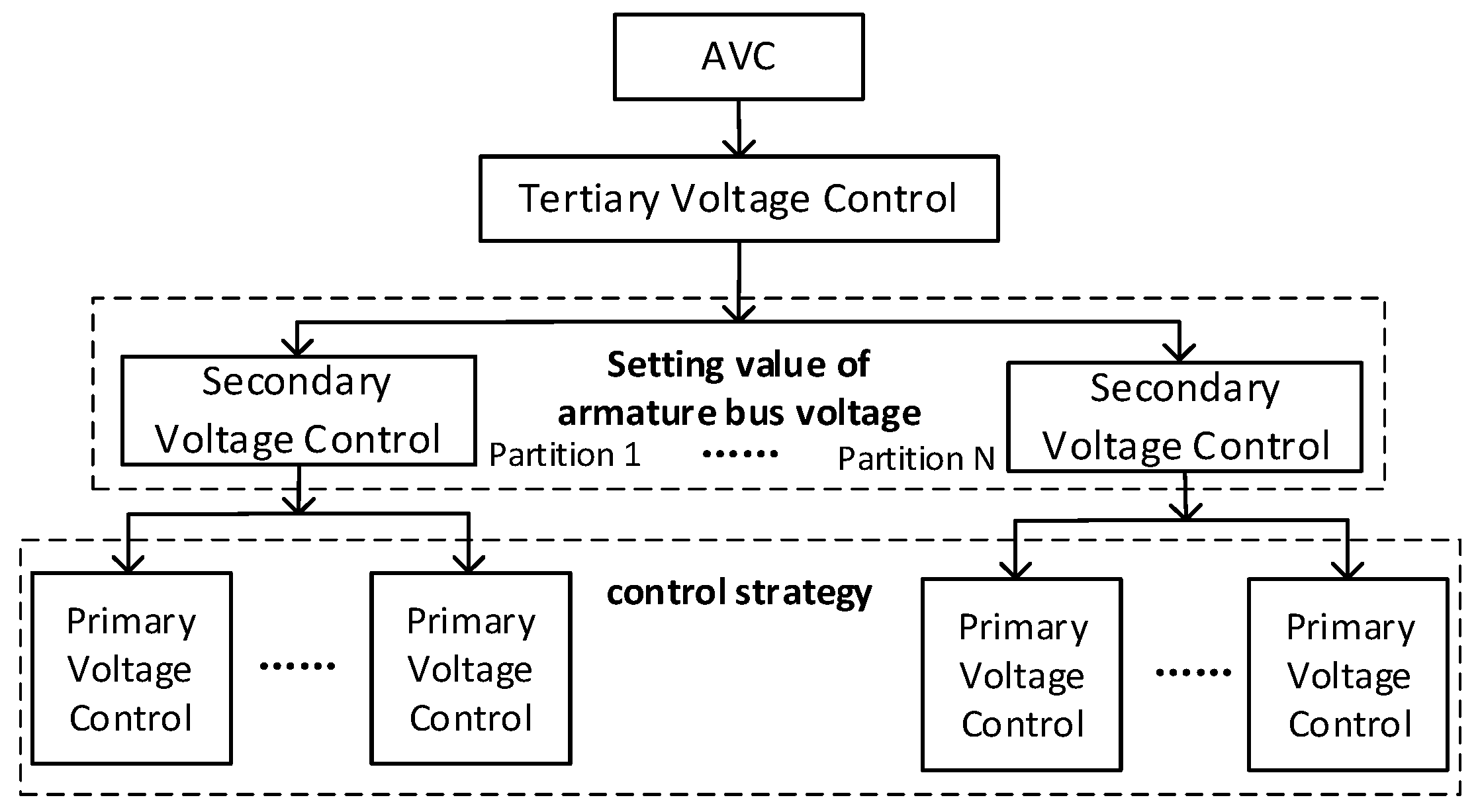
The AVC system collects real-time grid current information, analyzes the data, and processes them. By integrating automatic network partitioning, the system derives optimal calculation results and regulates the controlled units of the network to achieve optimal operation. The calculation process is executed sequentially, following the order of tertiary voltage control, secondary voltage control, and primary voltage control. The processes corresponding to these three levels, as illustrated in Figure 1, include regional global control, substation partition control, and local unit control, in that order [25,27].
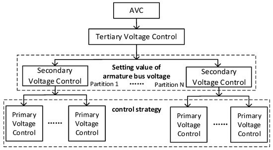
Figure 1.
AVC Control Block Diagram.
At the top level is the tertiary voltage control, also known as regional global control. It operates at an hourly level, aiming for global economic optimization. Reactive power optimization is employed to determine the set value of the armature bus voltage for each zone, which is then provided as a reference value to the secondary voltage control. The second level is the secondary voltage control, referred to as substation zone control. It operates on a minute-by-minute basis, maintaining the set value of the armature bus voltage in each zone as a reference. It generates reactive power requirements for the primary voltage control, which subsequently provides a reactive power reference value for the primary control. At the bottom level is the primary voltage control, also known as local control. The system utilizes locally collected current and switching data with a time resolution of seconds to control reactive power compensation devices, including On-Load Tap Changers (OLTCs), Synchronous Compensators (SCs), Static Var Generators (SVGs), and distributed renewable energy sources, thereby compensating for reactive power–voltage variations in the region.
2.2. Cooperative Reactive Power Optimization Model for Main and Distribution Networks
Cooperative reactive power optimization of the main and distribution networks primarily involves the overall optimization objective of three-level voltage control, typically applied to grids ranging from 220 kV to 35 kV. Renewable energy stations centrally connected to the grid at low voltage are integrated into low-voltage buses using an equivalent model, thereby establishing a reactive power optimization model for the main and distribution networks that incorporates distributed power sources in the regional distribution network. The optimal power flow calculation for reactive power optimization is performed to determine the target values for voltage optimization at all bus levels within the regional grid. Additionally, the reactive power optimization of the regional distribution network is incorporated, with the objective of achieving secondary voltage control.
2.2.1. Mathematical Models for Reactive Power Optimization
The global voltage–reactive power optimization calculation, as the highest level of the grid’s automatic voltage control system, is responsible for decision-making tasks, providing the system with an optimization scheme for the entire network. It aims to optimize the economic operation of the entire system, incorporates security indices, and provides the set reference values for busbar voltage optimization to support control decision-making [28]. The optimal power flow model is utilized for reactive power optimization calculations.
The optimal current reactive power optimization objective function is shown in (1).
where NL is the number of branches; Ploss is the active power network loss; Pij and Pji are the active power outflows from nodes i and j, respectively.
The equation constraints and inequality constraints satisfied are shown in (2) and (3), respectively.
where PG and QG are the active and reactive power of the power source; PD and QD are the active and reactive power of the load; Gij and Bij are the conductance and susceptance of the branch of nodes i and j; θij is the phase angle of the branch ij; QGmax and QGmin are the upper and lower limits of the reactive power output; Vmax and Vmin are the upper and lower limits of the voltage; tmax and tmin are the maximum and minimum values of the ratio of transformer with the on-load regulator tap; Ii,jmax is the maximum value of the safety current; NQG, NB, NT are the number of the reactive sources, the number of nodes, and the transformer gear, respectively. NL represents the set of nodes.
The reactive power sources mentioned above include reactive power equipment in substations at all levels, dispatched by the regional grid control center, as well as generators in power plants, renewable energy plants, and photovoltaic power stations under the jurisdiction of the control center. The strategy embedded in the mathematical model aims to identify the optimal operation method that minimizes active network losses across the entire network under var-voltage constraints.
For centralized grid-connected 110 kV renewable energy field stations within the regional grid, a coordinated secondary voltage control area is established, with the bus of the higher-level substation, which is pooled and connected to the grid, serving as the pivotal bus. Using the pivot bus voltage determined by global reactive power optimization as the target, adjustable reactive power regulation commands within the coordinated control area of 10 kV feeders are calculated and transmitted to the AVC substation for execution. Consequently, the secondary reactive power optimization mathematical model follows a similar approach, with the control objective of maintaining a constant regional bus voltage under tertiary voltage control and the control target being the 10 kV feeder reactive power optimization reference value.
2.2.2. Physical Equivalence Models for Optimization Equipment
- 1.
- Capacitors and Reactors
The capacitor reactive power of the substation needs to be considered in advance during the optimization process. Since capacitors and reactors are discrete regulation variables, directly incorporating them into the optimization model may compromise algorithm convergence and render them unsuitable for practical closed-loop control systems. Capacitors and reactors are controlled by serializing discrete device actions to derive an optimal strategy for reactive power and voltage distribution.
This is achieved by introducing a virtual regulator at the capacitor-connected bus, as illustrated in Figure 2. Similarly, for reactors, a virtual compensator can be substituted to enable continuous optimization.
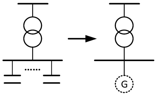
Figure 2.
Equivalent Modelling of Capacitors.
- 2.
- Centralized renewable energy stations
In the three-level voltage control reactive power optimization process, adjustable reactive power equipment (e.g., inverters and dynamic reactive power compensation devices) in centrally grid-connected renewable energy field stations operating at 35 kV to 110 kV should be included in the reactive power optimization framework.
Due to the large number of wind turbine generators (WTGs) and PV inverters in wind farms and PV plants, it is impractical to model each WTG and inverter individually in the dispatch center. Therefore, an equivalent model for the renewable energy field station and PV power station must be established and incorporated into the global reactive power optimization framework.
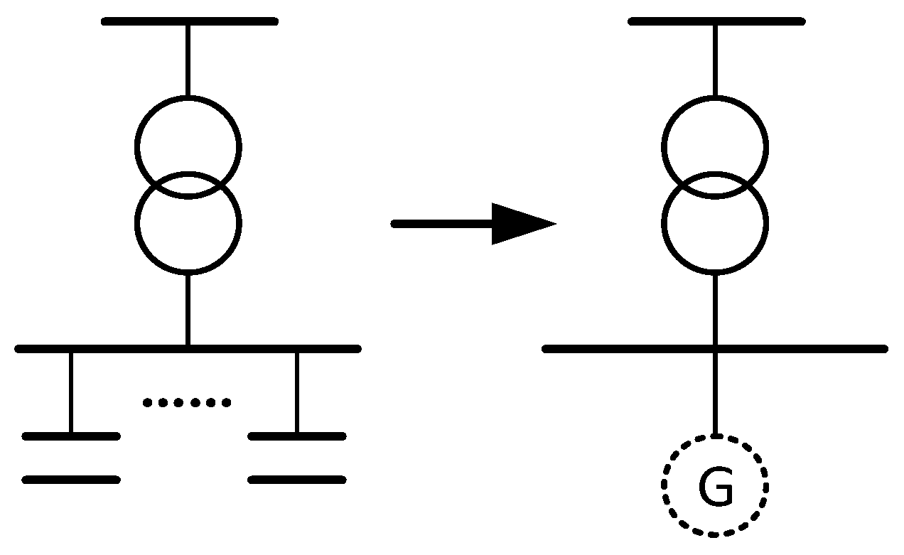
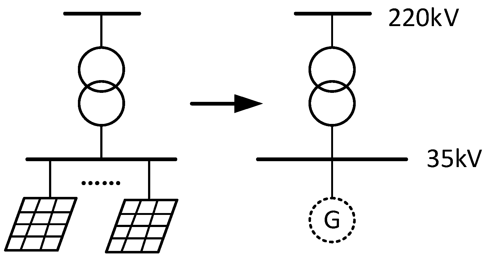
In a renewable energy field station, the dynamic reactive power compensation devices and PV arrays connected to the low-voltage side are controlled by the AVC substation within the PV power station. Consequently, an equivalent machine model for reactive power regulation is established on the 35 kV or 10 kV bus on the LV side of the renewable energy field station. This model is treated as a generator capable of providing additional reactive power during optimal power flow calculations for reactive power optimization, with the equivalence illustrated in Figure 3, using the PV field station as an example. The equivalence is based on the normal operating conditions of the PV system, and the reactive power margin of the PV system depends on the active power and total capacity at that moment, adhering to the Q–P curve.

Figure 3.
Equivalent modeling of PV stations.
- 3.
- Distributed renewable energy stations
The reactive power regulation capability of distributed energy sources is incorporated into the regional distribution network’s reactive power optimization process. Distributed energy sources are modeled as an equivalent machine capable of flexibly regulating both active and reactive power, as illustrated in Figure 4.
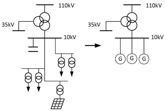
Figure 4.
Equivalent modeling of distributed energy.
2.3. Cross-Approximation Algorithm
2.3.1. Theory of Cross-Approximation Algorithms
The cross-approximation algorithm is a numerical method for solving large-scale coefficient linear systems [29]. The calculations are based on optimal power flow using the cross-approximation algorithm. Leveraging the weak coupling between active and reactive components inherent in power systems, the optimal power flow solution is obtained using active–reactive decoupled cross-approximation, grounded in the theory of convex and partial dyads.
By expressing the active and reactive relationship variables in terms of xp, xq, the description for the tidal current problem is shown in Equations (4) and (5).
where xp contains generator active PG and nodal voltage phase angle θ; xq includes the reactive power supply output QG, the nodal voltage magnitude V, and the adjustable transformer ratio t; PE and QE are the nodal active and reactive power flow equations, respectively; PI and QI are inequality constraints for the active and reactive components, respectively.
If the initial value of the above function is close to the optimal value, the assumption condition of partial convexity is satisfied. Then, equate Equations (4) and (5) to form (6) or (7) according to the conclusion of convex and partial dyads.
Corresponding the λq, μq, λp, μp of the above two equations to the dyadic variables near the solution node converts a large problem into two subproblems to solve, which greatly reduces the constraints’ solution limitations. Since the values of the dyadic variables at the solution node cannot be predicted, a common method is to solve the two subproblems of Equations (6) and (7) alternately until the same xp and xq are obtained for both of them, that is, the optimal value is found.
Considering the absence of reactive constraints in Equation (6) and active constraints in Equation (7), it is proposed to take the reactive variable as a known quantity in Equation (6) and the active variable as a known quantity in Equation (7). This, in turn, simplifies the two subproblems, as shown in Equations (8) and (9).
By solving these two sub-problems, the same values for xp and xq are ultimately calculated, which serve as the final solution.
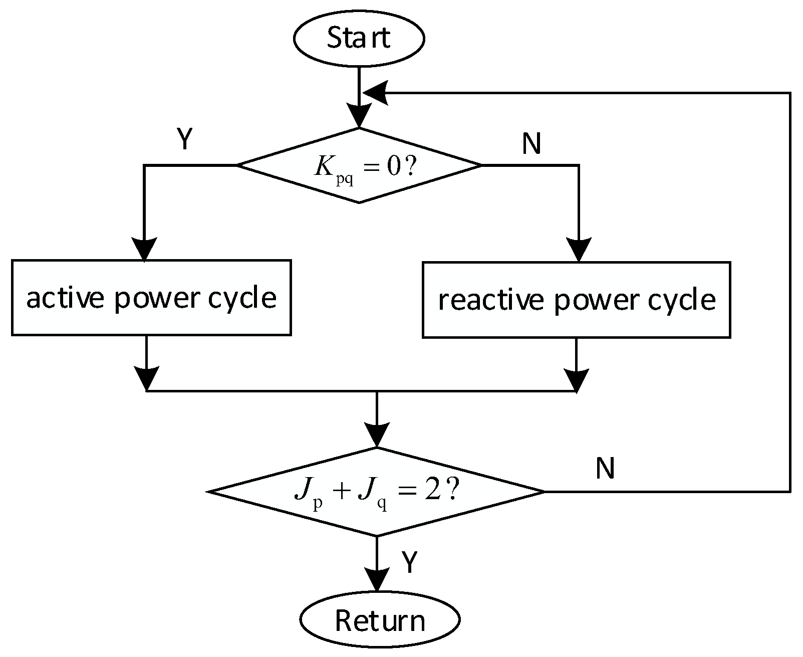
2.3.2. Flow of Cross-Approximation Algorithm
Figure 5 shows the computational flowchart of the cross-approximation algorithm. The first judgment box, Kpq, is the selection flag for active and reactive iteration. If its value is 0, then the iterative computation loop of the tactive sub-problem is carried out; if the value is 1, then the iterative loop of the reactive sub-problem is carried out. Jp and Jq in the second judgment box are the convergence flag bits of active and reactive powers, and the value of convergence is 1. When both sub-problems converge, if Jp = Jq = 1 and the sum of the two is 2, it indicates that the computation of optimal tidal current is completed, and the loop is exited afterward.
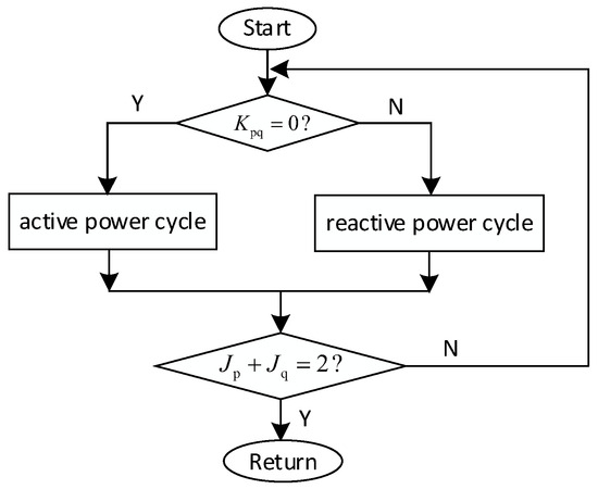
Figure 5.
Flowchart of the Cross-Approximation Algorithm.
The process computes the optimal power flow, leverages active–reactive decoupling, exhibits rapid convergence, and accurately accounts for various constraints. It demonstrates strong stability and has been successfully applied and refined in numerous engineering applications.
3. Local Var-Voltage Cooperative Control Method
At the regional distribution network level, the allocation of reactive power demand for primary voltage control is based on the two-stage objectives of tertiary and secondary voltage control reactive power optimization.
At the primary voltage control level, a two-stage decision-making method is proposed. In the first stage, the reactive power regulation strategy for each 10 kV feeder in the distribution network’s AVC is calculated. This is achieved by using the optimal 10 kV bus voltage value from the global reactive power optimization of the main distribution network as the target and leveraging the reactive power regulation capability of each 10 kV feeder provided by the distribution network’s AVC as the regulation mechanism. In the second stage, the distribution network’s AVC constructs a control model using the 10 kV feeder coordinated control area as the basis. The total reactive power setpoint of the feeder area’s root node, calculated by the local regulator AVC, serves as the target, while the voltage compliance of each loaded substation acts as a constraint. This enables the computation of reactive power regulation instructions for the new adjustable sectionalized energy sources within the 10 kV feeder’s coordinated control area. These instructions are then transmitted to the AVC substation for execution.
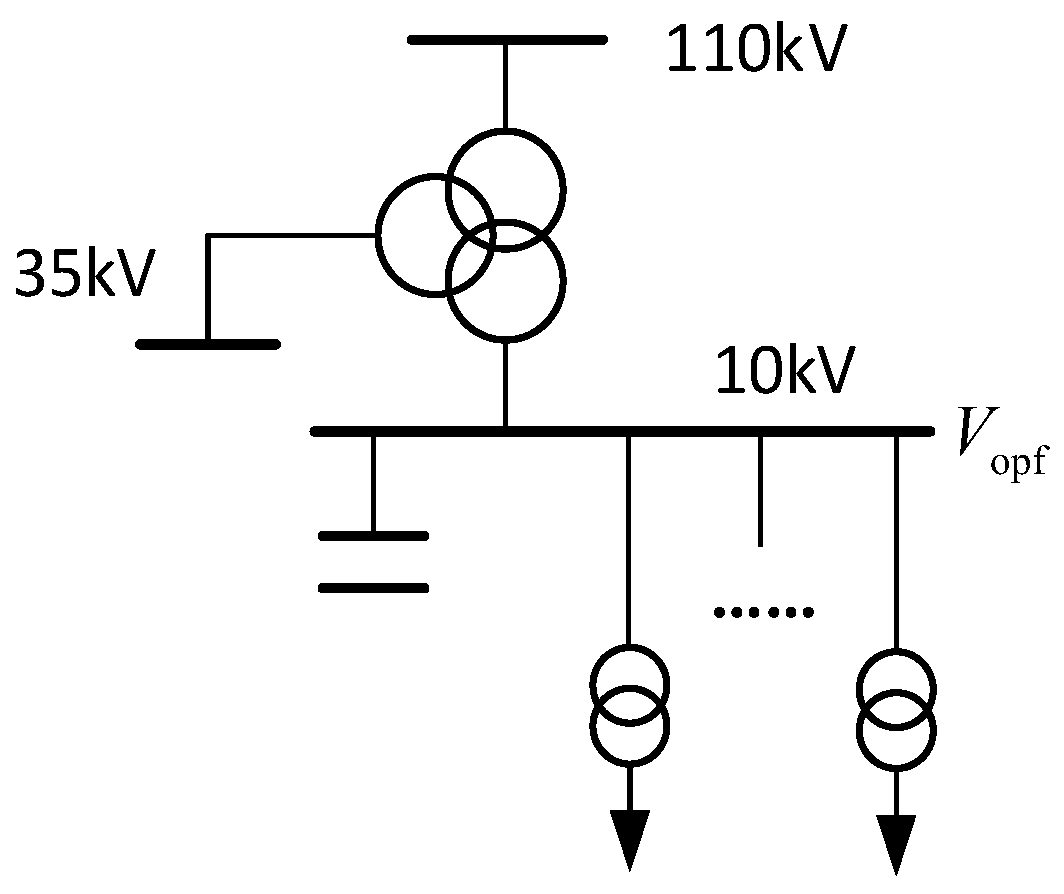
3.1. Reactive Power Control Program for 10 kV Feeder Lines
The first stage of decision-making focuses on the reactive power allocation for each feeder connected to the 10 kV bus, as illustrated in Figure 6. In order to meet the reference value of 10 kV bus voltage optimization Vopf issued by the superior AVC system, it is necessary to control the reactive power allocation of the feeders with reactive power regulation capability connected to the 10 kV bus (including the buses operating in parallel). The 10 kV feeder buses include the load profiles of the station transformers they are connected to, as well as adjustable reactive power resources, such as distributed photovoltaic systems and energy storage systems supported by the station transformers.

Figure 6.
Decision-making model for the first stage.
The active and reactive power outputs of each feeder group are obtained through the ground-based Energy Management System (EMS), and the reactive power threshold available from each station area at any given moment is calculated. The reactive power regulation range of each feeder is transmitted to the distribution network AVC via the station AVC substation, aggregated into the feeder (group) object, and used to determine the current reactive power upper limit Qmax and reactive power lower limit Qmin.
In order to determine the magnitude of reactive power to be supplied by each feeder carried by the 10 kV bus, quadratic programming is carried out for it, and a quadratic planning model is established, as shown in (10).
where Vj is the voltage detection value of the jth bus of 10 kV; Vopf,j is the voltage optimization value of the jth bus; Ωj is the set of feeders connected to the 10 kV bus; ΔQi is the reactive power adjustment amount of the feeder; Cvj is the var-voltage sensitivity of the jth bus; Wv and Wq are the weight values of the voltage target and reactive power equalization target, respectively; generally, the voltage target comes first and takes the values of 1.0 and 0.1, respectively; Riw is the reactive power adjustment equalization index of feeder i, which is defined as shown in (11).
where Qi is the reactive power injection value of feeder i; Qimax and Qimin are the upper and lower limits of reactive power regulation for this feeder, respectively.
The optimization constraints based on this model are shown in (12).
This method limits the 10 kV bus voltage and the reactive power regulation capability of the feeder group to the specified upper and lower limits.
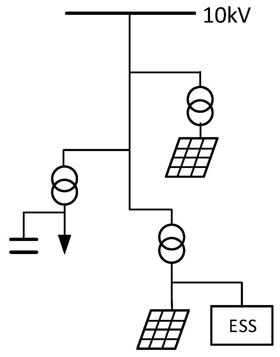
3.2. Reactive Power Control Program for Station Areas
The decision object in the second stage is the reactive power output of each 10 kV feeder at each station variable (group), as shown in Figure 7.

Figure 7.
Decision-making model for the second stage.
In the second stage of decision-making, the control target is the reactive power setpoint of the 10 kV feeder, determined during the first stage of decision-making. The control target is the reactive power injection of each 10 kV substation. The second stage focuses on the 10 kV feeder coordination and control area proposed in this study. Each area comprises one or more parallel-operating 10 kV feeders, along with the loads of the substations they serve. The reactive power resources primarily include distributed PV systems, energy storage systems (ESS), and conventional capacitors connected to the low-voltage side of the substation.
The current active and reactive power outputs of the 10 kV feeder (group) can be obtained from the local EMS. The current reactive power outputs of each substation (group) and the reactive power regulation capacity, i.e., the upper limit of reactive power and the lower limit of reactive power are calculated in real time by the AVC sub-station of the substation area and sent up.
In the second stage of decision-making, not only is the var-voltage compensation effect considered, but also the active network loss of the 10 kV feeder area. By solving the sensitivity Cl of the reactive power injection of the station transformer to the active network loss of the 10 kV feeder (group), the index of the influence of the reactive power regulation of the station area on the active network loss of the 10 kV feeder group can be obtained, so as to realize the reduction in the network loss through the reactive power regulation of the station area.
The quadratic programming model of a 10 kV feeder is constructed as shown in Equation (13).
where is the detected reactive power value of the root node of the 10 kV feeder; is the reactive power setpoint of the root node of the feeder, provided by the decision in the first stage; Ωj is the set of feeders connected to the 10 kV bus; ΔQi is the reactive power adjustment amount of the feeder; Cqj is the sensitivity of injected reactive power of the jth station area to the reactive power of the root node of the 10 kV feeder; is the current active network loss value of the 10 kV feeder group area; Clj is the sensitivity value of reactive power adjustment for active network loss in the ith 10 kV station area; Wq and Wl denote the weights of voltage target and reactive power equalization target, respectively, and, generally, the voltage target is taken as the first one, with the values of 1.0 and 0.1, respectively.
The constraints are shown in Equation (14).
where k is the number of the node of the 10 kV bus, and i is the station number. The total reactive power regulation capability of the 10 kV transformer is restricted to the specified upper and lower limits.
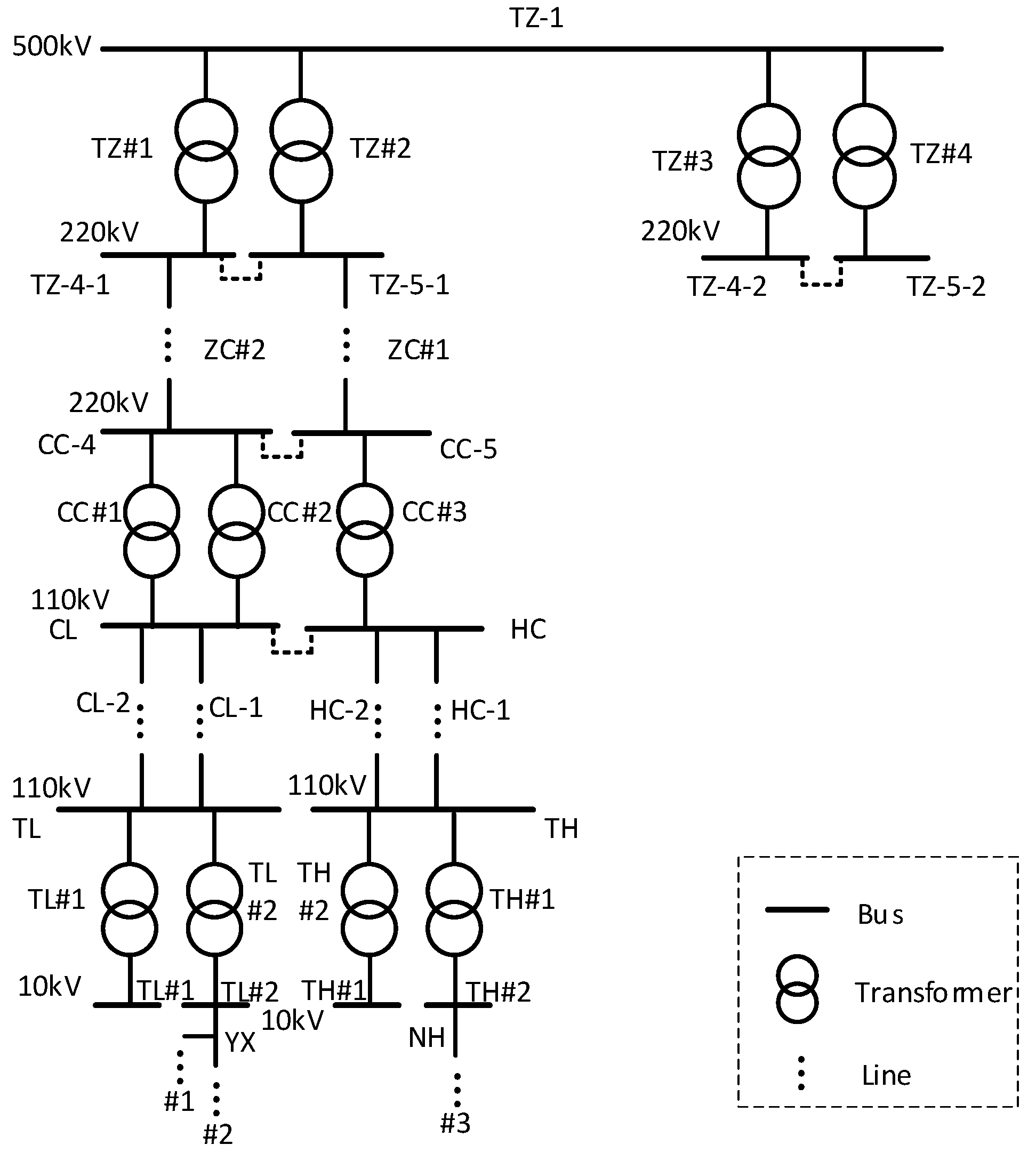
4. Example Analysis
The main distribution regional grid of a city containing distributed PV is selected for a three-level voltage reactive power optimization study, and the grid structure is shown in Figure 8. The grid includes four 500 kV substation main transformers, three 220 kV substation main transformers, four 110 kV substation main transformers, and several bus nodes. The 10 kV YX and NH lines serve as feeders connected to two and one distributed PV plants, respectively. These PV systems are capable of providing reactive power. The reactive power from these distributed PV systems can be utilized for local voltage control. All PV inverters comply with grid standards (IEEE 1547 [30] and IEC 61727 [31] and so on), featuring low-voltage ride-through (LVRT) and high-voltage ride-through (HVRT) capabilities, as well as protection functions. They operate within the specified voltage and frequency ranges.

Figure 8.
Structure of the regional power grid.
Operating data from a specific moment on a day in May 2024 are selected as a snapshot for analysis to establish an AVC control model for the regional distribution network. The active and reactive power values for feeders YX and NH are presented in Table 1. And the reactive power flowing from the grid to the load is defined as positive. On the YX feeder, the two photovoltaic (PV) stations are labeled #1 and #2, with reactive power margins of ±5 Mvar and ±6 Mvar, respectively, at the given time. On the NH feeder, the PV station is labeled #3, with a reactive power margin of ±10 Mvar. The PV inverters have a short response time, ranging from a few hundred milliseconds from receiving the AVC command to actual output adjustment. This response time has a minimal impact on grid stability. The power flow of the network at this moment is shown in Appendix A. The busbar voltage at this moment is measured, and the results are displayed in Table 2. The optimization algorithm involved is based on a self-developed calculation software, the TH2100 Grid Energy Management Platform, implemented in C++23.

Table 1.
The active and reactive power of feeders YX and NH.
Table 2.
Measured and optimized busbar voltages.
4.1. Tertiary and Secondary Voltage Optimization of Main and Distribution Networks
The cross-approximation algorithm is used to optimize the tertiary and secondary voltages, and the reference value of each busbar voltage of 10 kV and above is obtained by integrating economy and safety. The initial values for the cross-approximation calculation are selected as the bus voltage values from the previous time step. The calculated optimization results are shown in Table 3.
Table 3.
Network Ploss values before and after optimization.
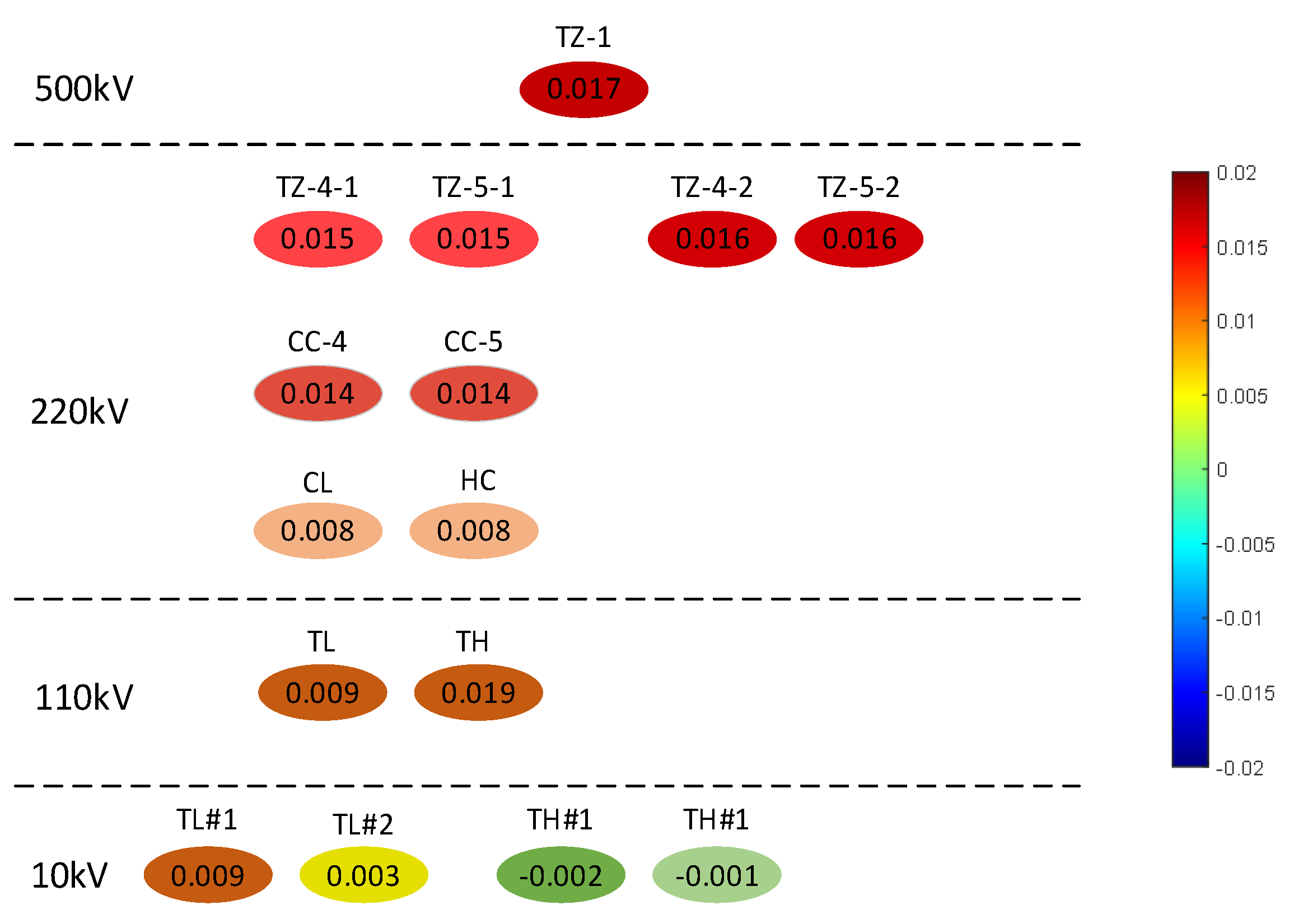
It can be seen that there is a slight difference between the optimized bus voltage values and the actual values. As seen in Table 3, the optimized network loss is reduced by 171.14 kW compared to the pre-optimized network loss. Figure 9 shows the per-unit value of voltage variation before and after optimization. It can be seen that through global reactive power optimization, the voltage value of the 500 kV busbar can be improved, which conforms to the trend of the whole network loss reduction. The voltage value resulting from the optimization is transmitted to the local reactive power control link as a voltage reference by AVC.
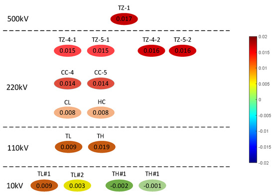
Figure 9.
Heat map of optimized voltage variation.
4.2. Primary Reactive Power Optimization in the Local Area
Consider the YX feeder carried by bus TL#2 and the NH feeder carried by bus TH#2 as the 10 kV feeders participating in the distribution network AVC control. Under the initial state, the root node voltage of the two buses and their power measurements are shown in Table 1. The YX feeder is connected to two distributed PV stations, designated as #1 and #2. The NH feeder is connected to a single distributed PV station labeled #3. The initial voltage, power, and power meter regulation capability of each station are shown in Table 4. U, P, and Q represent the measured values of voltage, active power, and reactive power, respectively. P margin and Q margin denote the ranges of active power variation and reactive power regulation, respectively. Both active and reactive power values are positive when power flows from the 10 kV bus to the load.
Table 4.
Voltage and power regulation capability for each station.
Based on the obtained optimized 10 kV bus voltage values, the voltage regulation amount for each feeder is obtained, as shown in Table 5. Based on the voltage value to be regulated, the reactive power adjustment amount for each group of feeders is solved using quadratic programming, as shown in Table 6.
Table 5.
Adjustment value of bus voltage.
Table 6.
Total reactive power regulation value for each feeder.
Through the total reactive power adjustment demand of each feeder, the quadratic programming is used to obtain the specific reactive power adjustment quantity issued to each substation, as well as the corresponding voltage adjustment quantity and target value, and the results are shown in Table 7.
Table 7.
Reactive power and voltage values of the station.
As indicated in Table 7, the required reactive power adjustments for station #1 and station #2 on feeder YX are −1.3244 kvar and −5.9764 kvar, respectively. For station #3 on feeder NH, the required reactive power adjustment is 10 kvar.
The reactive power output of each PV station is adjusted based on the planned reactive power adjustments, ensuring that the feeder reactive power aligns with the values calculated during the first stage of local optimization. This ensures that the busbar voltage under local control remains constant at the reference value specified by the secondary voltage control.
5. Conclusions
In this paper, a coordinated volt-var control method for the main and distribution networks is proposed, incorporating the reactive power regulation capability of load-side distributed PV systems. This method is summarized as follows:
- Coordinated optimization of the main and distribution networks is performed based on AVC tertiary and secondary voltage control. Tertiary control aims to minimize network losses across the entire system, optimizing and calculating reference values for bus voltages at all levels. Secondary voltage control optimizes the voltage values of buses with reactive power regulation capability, aiming to maintain the bus voltages at the optimized values determined in the previous stage. Reactive power optimization in the actual grid adjusts the voltage at each node, reducing network losses by 171.14 kW;
- Based on AVC primary voltage control (local control), the required reactive power adjustments for distributed PV resources in the station area are determined, and control commands are issued through the AVC system. This process is divided into two stages. In the first stage, the reactive power adjustment for each feeder is calculated using quadratic programming based on the bus voltage reference value. In the second stage, the total reactive power of each feeder root node is used as the target, with the voltage of each new energy substation serving as a constraint. The regulated reactive power adjustment commands for the adjustable distributed energy resources in the feeder area are calculated and transmitted to the AVC substation for execution;
- The proposed collaborative reactive power optimization method for main and distribution networks incorporates the global grid area, including 10 kV buses of regional grids, which are not addressed by traditional AVC systems. It also accounts for the reactive power regulation capability of centralized and distributed renewable energy field stations, reduces reliance on reactive power equipment, and enables integrated volt-var control across the main and distribution networks. However, the optimization algorithm utilized in this paper is relatively basic. The proposed optimization method can only maintain voltage optimization and has not yet achieved the maximization of distributed PV reactive power resources. The data selected are constrained by network and time limitations. In the future, more detailed research will be conducted to address these shortcomings.
Author Contributions
Methodology, Q.C.; software, H.W. (Haiyun Wang); validation, H.W. (Huayue Wei); investigation, H.W. (Haiyun Wang); resources, Z.Z. and H.W. (Huayue Wei); data curation, Q.C.; writing—original draft preparation, L.Z.; writing—review and editing, X.Y.; visualization, Z.Z.; supervision, X.C. All authors have read and agreed to the published version of the manuscript.
Funding
This research was funded by State Grid Beijing Electric Power Company, grant number 52022323000W. The APC was funded by State Grid Beijing Electric Power Company.
Data Availability Statement
The original contributions presented in this study are included in the article; further inquiries can be directed to the corresponding author.
Conflicts of Interest
Authors Haiyun Wang, Qian Chen, Zhijian Zhang, Huayue Wei were employed by the company State Grid Beijing Electric Power Company Electric Power Scientific Research Institute. The remaining authors declare that the research was conducted in the absence of any commercial or financial relationships that could be construed as a potential conflict of interest.
Appendix A
Table A1 presents the network power flow conditions at the optimization moment, including the specific values of active and reactive power on the high and low-voltage sides of each main transformer.
Table A1.
The power flow condition of the transformer.
Table A1.
The power flow condition of the transformer.
| Transformer Name | P/MW | Q/Mvar |
|---|---|---|
| TZ1 (high-voltage side) | 352.9135 | 1.6961 |
| TZ1 (low-voltage side) | 5.5673 | −0.0907 |
| TZ2 (high-voltage side) | 341.4900 | 47.9024 |
| TZ2 (low-voltage side) | 6.2065 | 110.0793 |
| TZ3 (high-voltage side) | 98.1261 | 25.8188 |
| TZ3 (low-voltage side) | 10.2178 | 50.8118 |
| TZ4 (high-voltage side) | 96.2783 | 14.5067 |
| TZ4 (low-voltage side) | 10.5796 | 55.5427 |
| CC1 (high-voltage side) | 35.5843 | 6.4662 |
| CC1 (low-voltage side) | −8.9728 | 1.7594 |
| CC2 (high-voltage side) | 36.1985 | 6.1547 |
| CC2 (low-voltage side) | −0.5269 | −2.6389 |
| CC3 (high-voltage side) | 40.1640 | 6.7231 |
| CC3 (low-voltage side) | −1.3727 | −3.0861 |
| TL1 (high-voltage side) | 2.3035 | 4.8457 |
| TL1 (low-voltage side) | −1.1741 | −1.8530 |
| TL2 (high-voltage side) | 7.3293 | 4.6137 |
| TL2 (low-voltage side) | −4.2407 | −1.8078 |
| TH1 (high-voltage side) | 10.0225 | 5.5012 |
| TH1 (low-voltage side) | 4.2400 | 1.8100 |
| TH2 (high-voltage side) | 10.4686 | 6.9329 |
| TH2 (low-voltage side) | 5.2301 | 3.1800 |
References
- Gulzar, M.M.; Iqbal, A.; Sibtain, D.; Khalid, M. An innovative converterless solar PV control strategy for a grid connected hybrid PV/wind/fuel-cell system coupled with battery energy storage. IEEE Access 2023, 11, 23245–23259. [Google Scholar] [CrossRef]
- Huang, N.; Zhao, X.; Guo, Y.; Cai, G.; Wang, R. Distribution network expansion planning considering a distributed hydrogen-thermal storage system based on photovoltaic development of the Whole County of China. Energy 2023, 278, 127761. [Google Scholar] [CrossRef]
- Shafiullah, M.; Ahmed, S.D.; Al-Sulaiman, F.A. Grid integration challenges and solution strategies for solar PV systems: A review. IEEE Access 2022, 10, 52233–52257. [Google Scholar] [CrossRef]
- Subramanian, K.; Loganathan, A.K. Voltage stability analysis of smart distribution grids with PV systems using fuzzy logic controller with firefly optimisation algorithm. Int. J. Eng. Syst. Model. Simul. 2023, 14, 125–140. [Google Scholar] [CrossRef]
- Gui, Y.; Nainar, K.; Bendtsen, J.D.; Diewald, N.; Iov, F.; Yang, Y.; Blaabjerg, F.; Xue, Y.; Liu, J.; Hong, T.; et al. Voltage support with PV inverters in low-voltage distribution networks: An overview. IEEE J. Emerg. Sel. Top. Power Electron. 2023, 12, 1503–1522. [Google Scholar] [CrossRef]
- Wang, X.; Wang, L.; Kang, W.; Li, T.; Zhou, H.; Hu, X.; Sun, K. Distributed Nodal Voltage Regulation Method for Low-Voltage Distribution Networks by Sharing PV System Reactive Power. Energies 2022, 16, 357. [Google Scholar] [CrossRef]
- Ibrahim, S.; Cramer, A.; Liu, X.; Liao, Y. PV inverter reactive power control for chance-constrained distribution system performance optimisation. IET Gener. Transm. Distrib. 2018, 12, 1089–1098. [Google Scholar] [CrossRef]
- Zhang, H.; Shen, J.; Wang, G. Day-ahead stochastic optimal dispatch of LCC-HVDC interconnected power system considering flexibility improvement measures of sending system. Int. J. Electr. Power Energy Syst. 2022, 138, 107937. [Google Scholar] [CrossRef]
- Jiao, W.; Chen, J.; Wu, Q.; Li, C.; Zhou, B.; Huang, S. Distributed coordinated voltage control for distribution networks with DG and OLTC based on MPC and gradient projection. IEEE Trans. Power Syst. 2021, 37, 680–690. [Google Scholar] [CrossRef]
- Dimitropoulos, D.; Wang, X.; Blaabjerg, F. Stability impacts of an alternate voltage controller (avc) on wind turbines with different grid strengths. Energies 2023, 16, 1440. [Google Scholar] [CrossRef]
- Duan, J.; Shi, D.; Diao, R.; Li, H.; Wang, Z.; Zhang, B.; Bian, D.; Yi, Z. Deep-reinforcement-learning-based autonomous voltage control for power grid operations. IEEE Trans. Power Syst. 2019, 35, 814–817. [Google Scholar] [CrossRef]
- Nour, A.M.; Hatata, A.Y.; Helal, A.A.; El-Saadawi, M.M. Review on voltage-violation mitigation techniques of distribution networks with distributed rooftop PV systems. IET Gener. Transm. Distrib. 2020, 14, 349–361. [Google Scholar] [CrossRef]
- Wang, Z.; Wang, Y.; Liu, G.; Zhao, Y.; Cheng, Q.; Wang, C. Fast distributed voltage control for PV generation clusters based on approximate newton method. IEEE Trans. Sustain. Energy 2020, 12, 612–622. [Google Scholar] [CrossRef]
- Khan, M.A.; Haque, A.; Kurukuru, V.S.B. Reliability analysis of a solar inverter during reactive power injection. In Proceedings of the 2020 IEEE International Conference on Power Electronics, Drives and Energy Systems (PEDES), Jaipur, India, 16–19 December 2020; IEEE: Piscataway, NJ, USA, 2020; pp. 1–6. [Google Scholar]
- Collins, L.; Ward, J.K. Real and reactive power control of distributed PV inverters for overvoltage prevention and increased renewable generation hosting capacity. Renew. Energy 2015, 81, 464–471. [Google Scholar] [CrossRef]
- Rostami, S.M.; Hamzeh, M.; Nazaripouya, H. Distributed Cooperative Reactive Power Control of PV Systems with Dynamic Leader. IEEE Trans. Ind. Inform. 2024, 20, 8972–8982. [Google Scholar] [CrossRef]
- Moondee, W.; Srirattanawichaikul, W. Reactive power management of MV distribution grid with inverter-based PV distributed generations using PSO algorithm. In Proceedings of the IECON 2019-45th Annual Conference of the IEEE Industrial Electronics Society, Lisbon, Portugal, 14–17 October 2019; IEEE: Piscataway, NJ, USA, 2019; Volume 1, pp. 2239–2244. [Google Scholar]
- Graf, F.R. Real time application of an optimal power flow algorithm for reactive power allocation of the RWE energy control center. In Proceedings of the IEE Colloquium on International Practices in Reactive Power Control, London, UK, 7 April 1993; IET: London, UK, 1993; pp. 7/1–7/4. [Google Scholar]
- Lefebvre, H.; Fragnier, D.; Boussion, J.Y.; Mallet, P.; Bulot, M. Secondary coordinated voltage control system: Feedback of EDF. In Proceedings of the 2000 Power Engineering Society Summer Meeting (Cat. No. 00CH37134), Seattle, WA, USA, 16–20 July 2000; IEEE: Piscataway, NJ, USA, 2000; Volume 1, pp. 290–295. [Google Scholar]
- Paul, J.P.; Leost, J.Y.; Tesseron, J.M. Survey of the secondary voltage control in France: Present realization and investigations. IEEE Trans. Power Syst. 1987, 2, 505–511. [Google Scholar] [CrossRef]
- Lee, K.Y.; Park, Y.M.; Ortiz, J.L. A united approach to optimal real and reactive power dispatch. IEEE Trans. Power Appar. Syst. 1985, PAS-104, 1147–1153. [Google Scholar] [CrossRef]
- Qi, P.; Yang, X.; Zhuo, G. Design of three level voltage control system in distribution network with the connection of many distributed photovoltaic power plants. Power Syst. Prot. Control 2014, 42, 48–64. [Google Scholar]
- Liu, Y.; Zhang, L.; Zhao, D.; Wang, D.; Zhang, H. Study on control characteristic of grid-connected solar photovoltaic plant based on simulation. In Proceedings of the 2015 5th International Conference on Electric Utility Deregulation and Restructuring and Power Technologies (DRPT), Changsha, China, 26–29 November 2015; IEEE: Piscataway, NJ, USA, 2015; pp. 1954–1958. [Google Scholar]
- Zhao, Y.N.; Liu, Q.H.; Song, S.Y.; Mao, W. An improved AVC strategy applied in distributed wind power system. IOP Conf. Ser. Earth Environ. Sci. 2016, 40, 012064. [Google Scholar] [CrossRef]
- Xia, Y.; Su, Z.; Song, M.; Pan, W.; Zhao, Q.; Yu, P.; Cheng, Y. Researches on control strategy of distributed AVC for district grids. In Proceedings of the 2017 IEEE Conference on Energy Internet and Energy System Integration (EI2), Beijing, China, 26–28 November 2017; IEEE: Piscataway, NJ, USA, 2017; pp. 1–4. [Google Scholar]
- Liu, S.; Wei, H.C. Application of AGC/AVC in Photovoltaic Power Station. Appl. Mech. Mater. 2014, 614, 151–154. [Google Scholar] [CrossRef]
- Zhang, H.; Xiao, G.; Liu, Z.; Zhou, Y. Impedance-Based Stability Analysis and On-Site Stability Evaluation of Three-Phase Active Voltage Conditioner (AVC) Embedded System. IEEE Trans. Power Electron. 2023, 38, 16061–16071. [Google Scholar] [CrossRef]
- Zheng, W.; Wu, W.; Zhang, B.; Sun, H.; Liu, Y. A fully distributed reactive power optimization and control method for active distribution networks. IEEE Trans. Smart Grid 2015, 7, 1021–1033. [Google Scholar] [CrossRef]
- Kishore Kumar, N.; Schneider, J. Literature survey on low rank approximation of matrices. Linear Multilinear Algebra 2017, 65, 2212–2244. [Google Scholar] [CrossRef]
- IEEE Std 1547; IEEE Standard for Interconnection and Interoperability of Distributed Energy Resources with Associated Electric Power Systems Interfaces. IEEE: Piscataway, NJ, USA, 2018.
- IEC 61727; Photovoltaic (PV) Systems—Characteristics of the Utility Interface. International Electrotechnical Commission: Geneva, Switzerland, 2004.

Disclaimer/Publisher’s Note: The statements, opinions and data contained in all publications are solely those of the individual author(s) and contributor(s) and not of MDPI and/or the editor(s). MDPI and/or the editor(s) disclaim responsibility for any injury to people or property resulting from any ideas, methods, instructions or products referred to in the content. |
© 2025 by the authors. Licensee MDPI, Basel, Switzerland. This article is an open access article distributed under the terms and conditions of the Creative Commons Attribution (CC BY) license (https://creativecommons.org/licenses/by/4.0/).