Abstract
In order to improve the current dynamic performance of induction motor (IM) drive systems, an internal model current decoupling control strategy is proposed to suppress the stator’s internal coupling effect. First, the IM mathematical model in the complex frequency domain is established, and the expressions of the coupling terms are derived. Then, according to the zero-pole distribution diagram and Bode plots, the design details for the structure and parameters of the internal model controller are presented in a continuous domain, and the impact of stator inductance mismatch on decoupling performance is analyzed. In addition to considering sampling and control delays, the IM mathematical model is established in the discrete domain, and the principle of the controller parameter is presented. Finally, the experimental results prove that the proposed internal model current decoupling control strategy can effectively improve the dynamic performance of IMs. Compared with the traditional feedforward current decoupling control strategy, the proposed method has superior decoupling performance under the operating conditions of low switching frequency. At the same time, a better steady-state performance is obtained by the proposed internal model control strategy.
1. Introduction
Induction motors (IMs) have advantages such as high efficiency, high torque output capability, and high reliability [1,2] and are widely used in industrial fields such as high-speed railways and electric vehicles [3,4]. Various control strategies for induction motors have also been proposed, including constant voltage frequency ratio control [5], vector control [6], direct torque control [7], and model prediction control [8]. Among them, vector control based on rotor flux orientation can achieve independent control of flux and torque, providing IMs with the speed regulation characteristics of DC motors [9], so it is currently the most mature and widely used motor control technology. However, after Clarke and Park’s transformation, there is a cross-coupling term in the mathematical model of the IM, which leads to an incomplete linear relationship between voltage and current in the d–q axis. In cases of high speed or parameter mismatch, the dynamic performance of the control system will deteriorate [10].
Feedforward decoupling compensates for the output voltage by adding a decoupling term to the reference of the stator current; this decoupling principle is simple, easy to implement, and widely used in engineering [11]. However, the cross-coupling in IMs is caused by the actual stator current, and the inconsistency between the exact value and the reference value may cause incomplete decoupling. In addition, the decoupling effect is poor under the conditions of low carrier ratio and parameter mismatch. In the literature [12], the state equation is transformed and a diagonalization matrix is constructed, so the linearization of the current control equation is achieved. According to the zero pole shift theory, the literature [13] introduces complex vector decoupling in the PI controller, improving decoupling performance in high-speed intervals. The literature [14] analyzes the impact of carrier ratio reduction on coupling effects; to improve the decoupling performance under a low carrier ratio, the delay compensation is introduced into the complex vector decoupling controller. In [15], a compensation angle is added to compensate for the angle delay, and a decoupling algorithm combining model predictive control is proposed to compensate for the time delay. However, the above methods rely on the accuracy of speed measurement and parameters, so the coupling effect cannot be decoupled completely.
The literature [16] considers voltage coupling an uncertain disturbance and adopts a disturbance observer (DOB) decoupling method. Although DOB decoupling is superior to diagonalization decoupling under inaccurate parameters, the decoupling performance is affected by nonlinear factors in the inverter. In [17], a sliding mode observer is adopted to estimate the stator current and feed it back to the input, achieving the decoupling of the d-axis and q-axis currents and solving the problem of poor robustness in feedforward decoupling. However, current oscillation occurs when the motor operates under high-speed conditions. The literature [18] proposes a current decoupling method based on an extended state observer (ESO), which obtains comprehensive observations and compensates for cross-coupling and disturbances caused by other factors through ESO to achieve decoupling. However, an increase in ESO bandwidth will reduce the stability of the control system. The literature [19] adopts an improved neural network algorithm for decoupling controllers, which improves the dynamic response speed, but the computational burden of the algorithm is too high.
Internal model decoupling is a mature control method developed from process control, which separates uncertain factors from the controlled object model [20]. It can dynamically track the reference and eliminate the influence of uncertain interference without a completely accurate model. Compared with other decoupling methods, internal model decoupling has the advantages of simple tuning and easy adjustment, and higher robustness can be obtained. This paper studies the parameter design methods of the internal model current decoupling controller in a continuous domain (s-domain). Then, to improve the decoupling performance under low switching frequency, the internal model current decoupling controller is modified in a discrete domain (z-domain). Finally, the experimental verifications are completed. The chapters are organized as follows: In Section 2, the d–q axis cross-coupling characteristic is analyzed based on the mathematical model of the IM. In Section 3, a current decoupling controller based on the internal model principle is proposed. In Section 4, the experimental results are presented. Finally, the conclusion is drawn in Section 5.
2. The Mathematical Model and Coupling Effect Analysis of the IM
This section first establishes the mathematical model of the induction motor, and on this basis, the expression of the complex vector transfer function is derived, and its coupling effect is analyzed.
2.1. Model of Induction Motor
Assuming that the magnetic potential generated by the stator and rotor in the air gap is sinusoidally distributed and ignoring the effects of ferromagnetic saturation, eddy currents, and teeth slots, the flux linkage and voltage equations of the squirrel-cage induction motor in the d–q coordinate system are expressed as follows [21]:
In the above two equations, ψsd and ψsq represent the stator flux linkage in the d-axis and q-axis, respectively, ψrd and ψrq represent the rotor flux linkage in the d-axis and q-axis, respectively, isd and isq represent the stator current in the d-axis and q-axis respectively, ird and irq represent the rotor current in the d-axis and q-axis, respectively, usd and usq represent the stator voltage in the d-axis and q-axis, respectively, urd and urq represent the rotor voltage in the d-axis and q-axis, respectively, Ls represents the stator inductance, Lm represents the excitation inductance, Lr represents the rotor inductance, Rs represents the stator resistance, Rr represents the rotor resistance, p represents the differential operator, ωe represents the synchronous angular frequency, and ωr represents the rotor electrical angular frequency.
In the d–q coordinate system, ψrq is equal to zero, and the rotor flux linkage ψr is equal to ψrd. According to Equations (1) and (2), the relationship between ψr and isd is obtained as follows:
where Tr is the rotor time constant, which is equal to Lr/Rr.
The spatial vectors are defined as follows:
where j represents the imaginary component, and us, ur, ψs, ψr, is, and ir donate spatial vectors of state voltage, rotor voltage, stator flux linkage, rotor flux linkage, stator current and rotor current, respectively. Then, the flux linkage equation of Formula (1) and the voltage equation of Formula (2) can, respectively, be expressed in the form of spatial vectors.
2.2. Coupling Effect Analysis
According to Equations (5) and (6), in the d–q coordinate system, the s-domain transfer functions of rotor flux linkage and stator voltage can be obtained as follows:
where s represents the complex frequency domain operator, ψs(s), Is(s), and Us(s) are the s-domain expressions of rotor flux, stator current, and stator voltage vectors, respectively, magnetic leakage coefficient σ = 1 − L2m/(LrLs), and stator equivalent resistance .
Substituting Equation (7) into Equation (8), the transfer function Gm_f(s) from the stator voltage us to the stator current is of the IM can be obtained as follows:
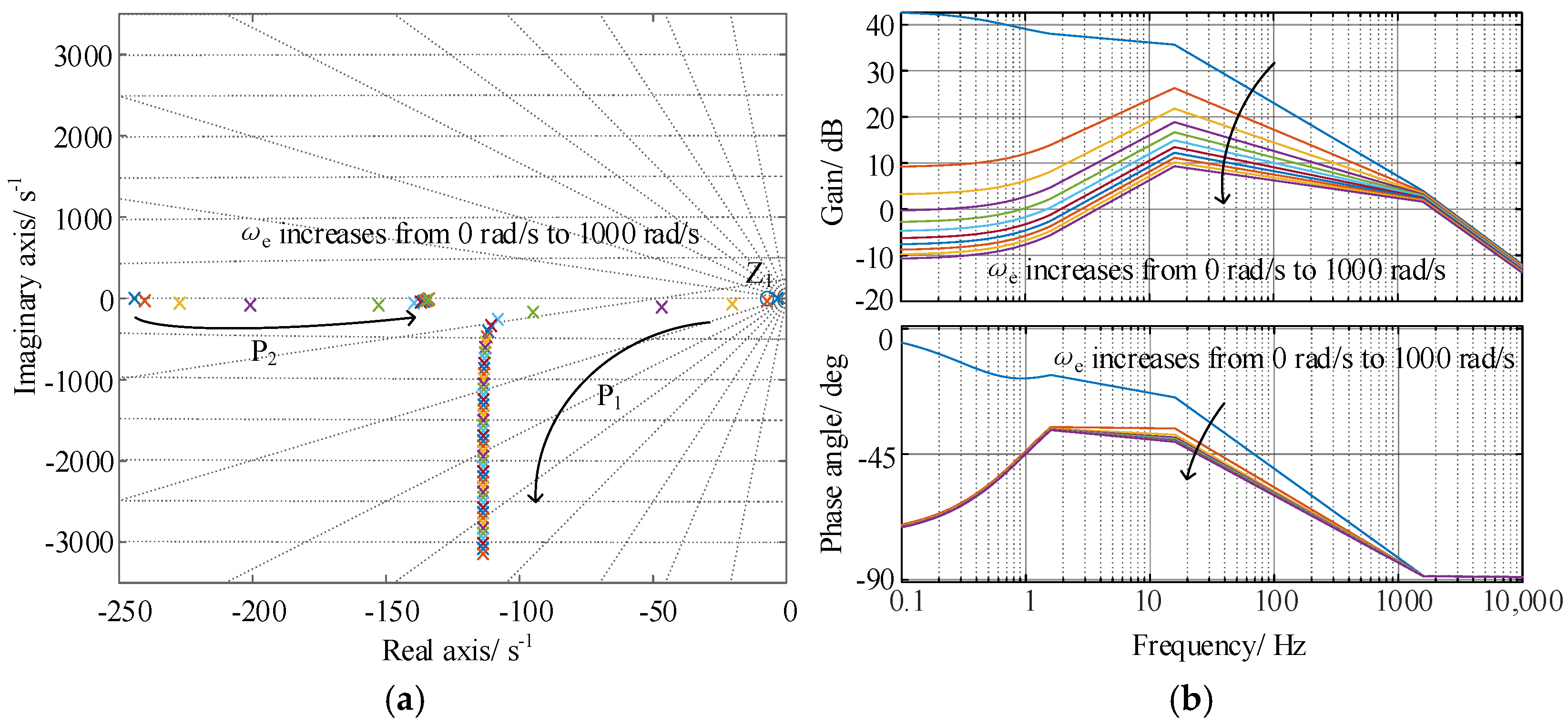
The parameters of the IM and inverter used in the theoretical analysis, simulation, and experiment are presented in Table 1. According to Equation (9), when the synchronous speed ωe rises from 0 to 1000 rad/s, the distribution of zeros and poles and the frequency characteristics are plotted in Figure 1. When ωe = 0 rad/s, Gm_f(s) has a pair of zeros, Z1, and poles, P1, that can cancel each other out, as well as a pole, P2, far from the imaginary axis. As the synchronous speed ωe increases, the imaginary axis component of pole P1 gradually increases, presenting a coupled and increasingly underdamped state, which leads to an increase in oscillations during the dynamic process.

Table 1.
Parameters of IMs and controllers.
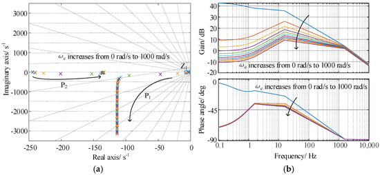
Figure 1.
Distribution of poles and zeros of Gm_f(s) when fe rises from 0 to 500 Hz. (a) Zero-pole distribution diagram. (b) Bode plots.
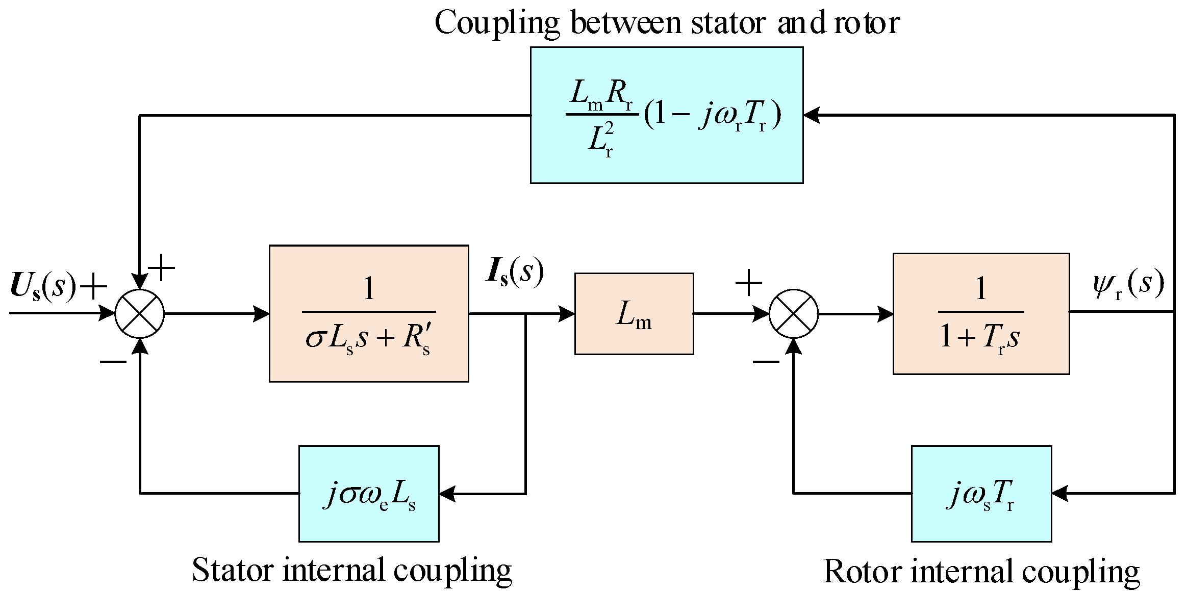
From Equations (7) and (8), the space vector structure diagram of the induction motor in the s-domain can be obtained, as shown in Figure 2.
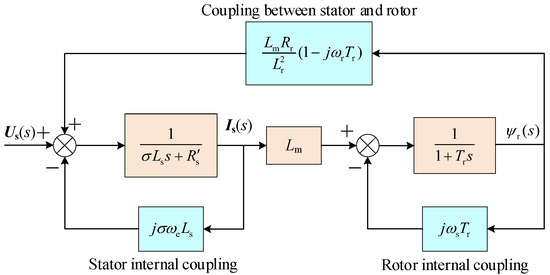
Figure 2.
Diagram of induction motor in s-domain.
The degree of current cross-coupling is determined by the imaginary component of the transfer function Gm_f(s). According to Figure 2, the coupling of the IM includes the following three parts:
- (1)
- Stator internal coupling : This is generated by the rotating coordinate transformationl the coupling degree is directly proportional to the synchronous angular frequency ωe and the stator current Is(s). Under the condition of high speed and large current, this coupling term has a significant impact on system performance;
- (2)
- The coupling term between the stator and rotor : This term is directly proportional to the rotor angular frequency ωr, and the coupling between the stator and rotor increases as the speed increases. According to Equation (7), the rotor flux ψr(s) lags behind the stator current Is, and this part of the coupling component can be regarded as an external disturbance to the system, which is considered as electromotive force Es(s);
- (3)
- Rotor internal coupling : Its magnitude depends on the slip frequency ωs, and the rotor flux ψr(s), and is related to the rotor time constant Tr. ωs is usually small, so this term has little effect on the dynamic performance of the IM. When the motor operates with no load and zero speed, there is no internal coupling in the rotor.
3. Internal Model Current Decoupling Controller for IM
Current coupling is considered an external disturbance, based on the theory of internal model control; the internal model current controller is first designed in the s-domain, then is discretized to reflect the characteristics of digital control, and the parameter optimization of the current decoupling controller is designed in the z-domain.
3.1. Design of Internal Model Current Decoupling Controller in Continuous Domain
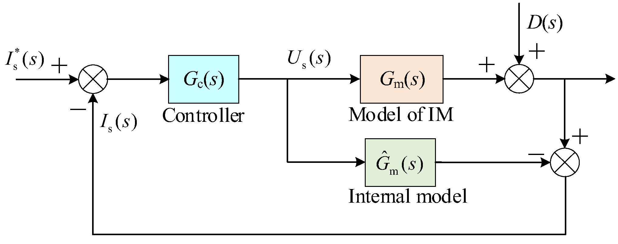
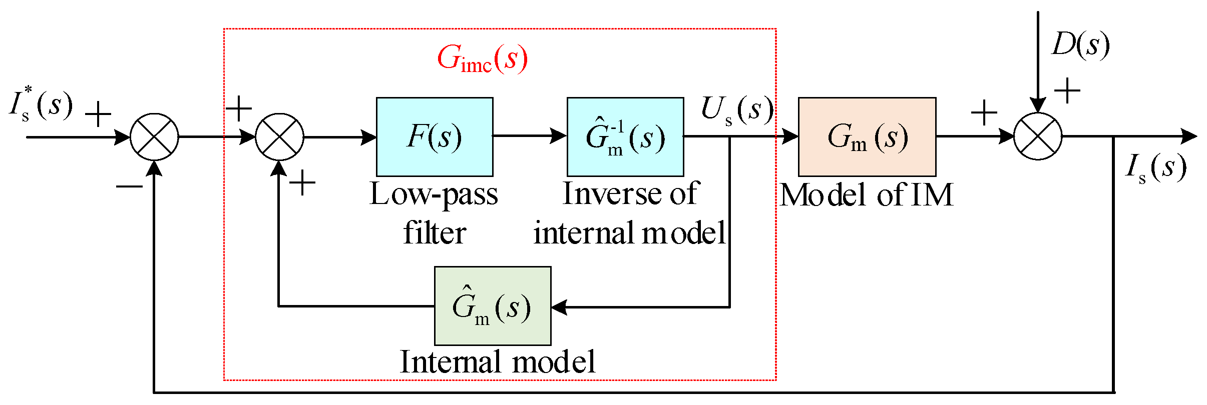
As shown in Figure 3, an s-domain current control system IM is designed based on the internal model control principle, where (s) represents the reference of the stator current, D(s) represents the current disturbance caused by coupling, Is(s) represents the actual stator current, Gm(s) is the first term of Equation (8), Ĝm(s) is the internal model, and Gc(s) is the controller to be designed.
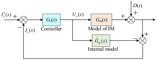
Figure 3.
Schematic diagram of internal model current control system in s-domain.
According to Figure 3, the Is(s) can be expressed as follows:
when , if , will be obtained. Therefore, if the model of the IM is accurate, it can overcome the interference and achieve zero-error tracking. From Equation (10), it can be obtained that , where symbol “ˆ” denotes the estimated value. It can be seen that the differential item occurs in Ĝm(s), a low-pass filter F(s) is introduced in the control loop, and its transfer function is defined as follows:
At this time, the transfer function of is expressed as follows:
The equivalent structure of the internal model control system is shown in Figure 4.
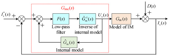
Figure 4.
Equivalent structure diagram of internal model control system.
According to Figure 4, the expression of the internal model current controller Gimc(s) is as follows:
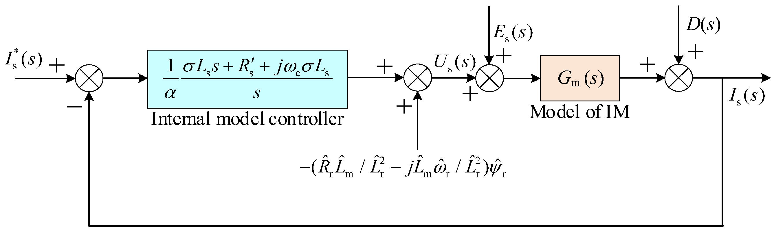
and the back electromotive force compensation term are introduced into the current loop. The complete structure of the s-domain internal model current control system is shown in Figure 5.
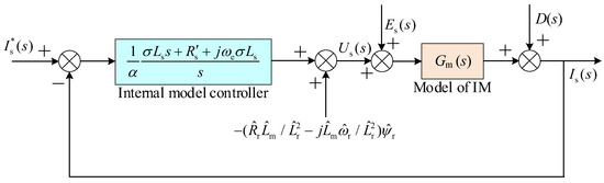
Figure 5.
Block diagram of current loop controlled by internal-model system.
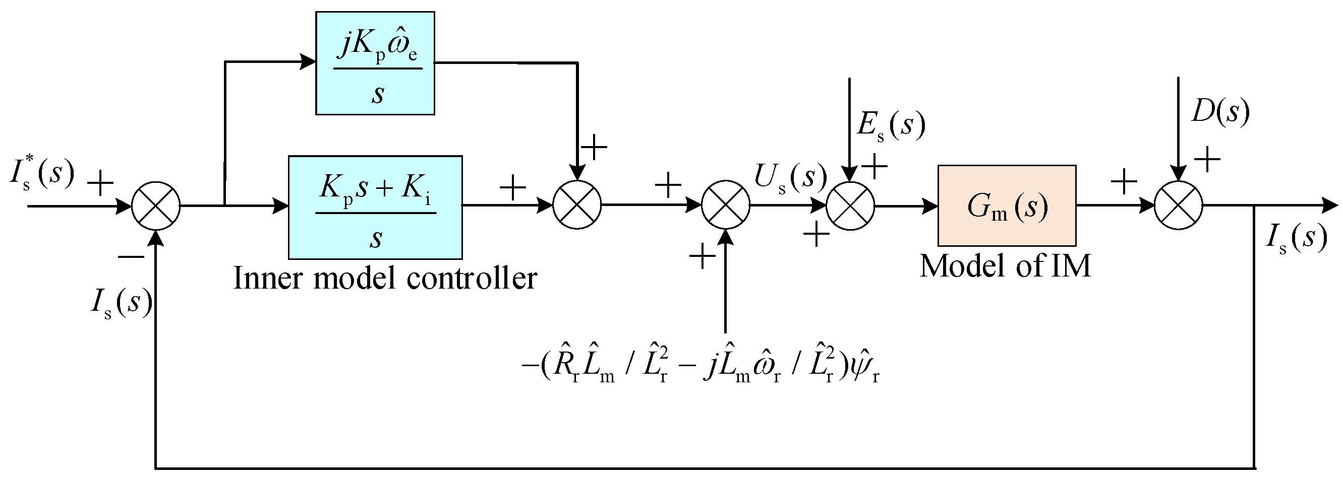
As shown in Figure 6, when , the internal model current controller can be regarded as a PI controller, Kp + Ki/s, with an added cross-decoupling term, jKp/s, and a back-EMF compensation term, . Combined with Figure 4, the cross-decoupling term in Figure 6 can eliminate the stator’s internal coupling, and the back-EMF compensation term can eliminate the influence of the coupling between the stator and rotor. Since the slip frequency is usually small, the influence of the rotor internal coupling can be ignored. Therefore, in the s-domain, the internal model current controller can completely decouple the d-axis and q-axis currents when the switching frequency is high.
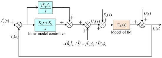
Figure 6.
Another form of internal-model decoupling.
When the internal model current controller is used, the current open-loop transfer function is expressed as (14). When the parameter is accurate, Go(s) is equal to ωb/s, and the system has no coupling, which verifies the above analysis.
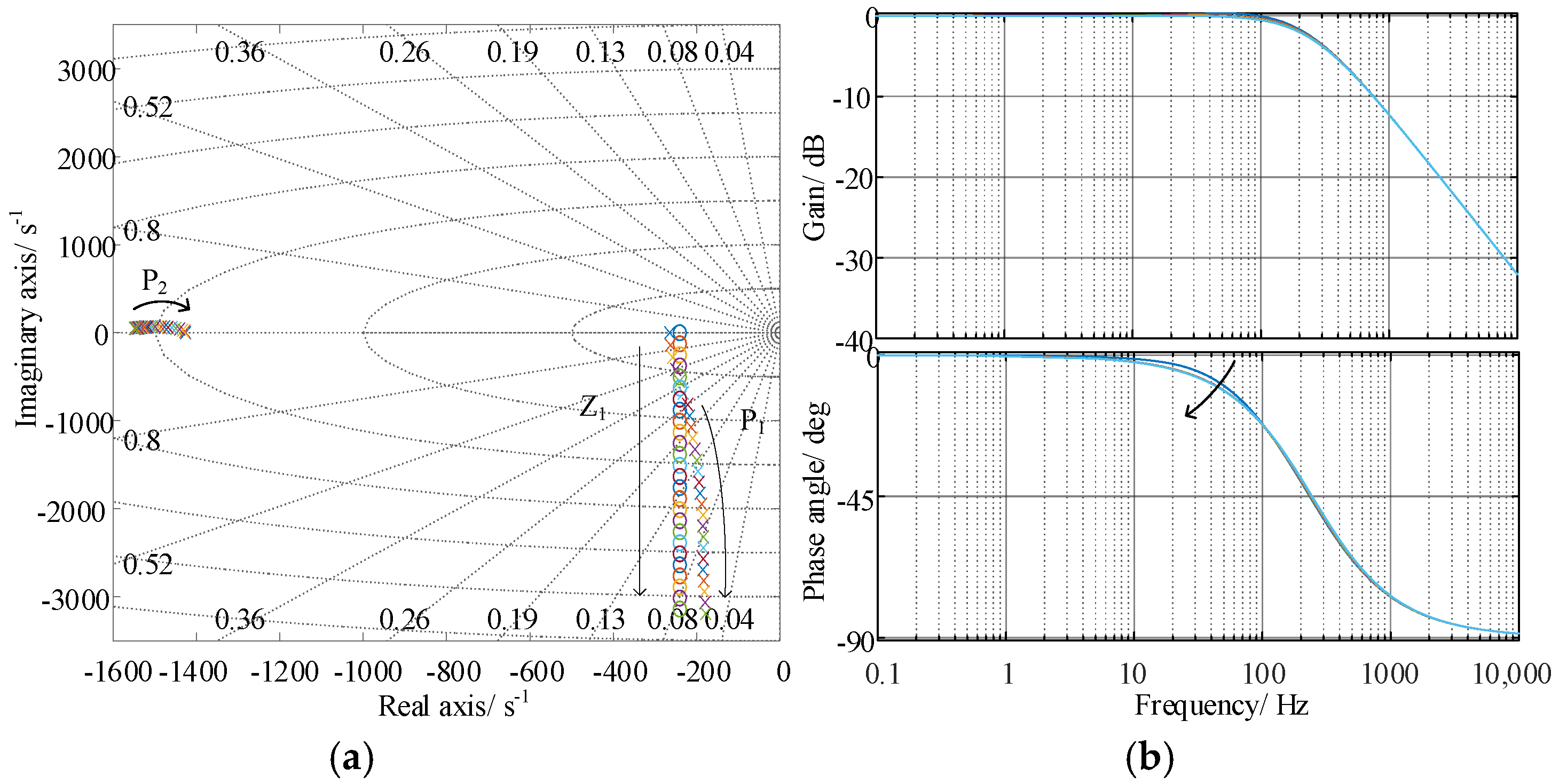
When synchronous speed ωe varies within the range of [0 rad/s, 1000π rad/s], and the internal model controller parameters are accurate, the zero-pole distribution diagram of the current closed-loop transfer function is drawn and shown in Figure 7. It can be seen that due to the cross-decoupling term , the internal model controller generates a zero Z1 at the same position as the pole P1, eliminating the internal coupling of the stator caused by the rotation coordinate transformation. The positions of Z1 and P1 are completely coincident, so the internal model controller can eliminate the increase in current control coupling and the decrease in system stability at high synchronous speed, and complete decoupling is achieved.
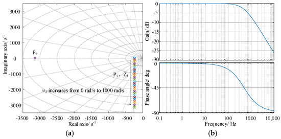
Figure 7.
The pole-zero distribution diagram and Bode plots of the internal model system. (a) Closed-loop zero-pole distribution diagram. (b) Closed-loop Bode plots.
When , the zero and pole distribution of the current closed-loop transfer function under the internal model controller is shown in Figure 8a. Compared with Figure 7a, as the synchronous speed ωe increases, there is a slight position deviation between the zero Z1 and pole P1. However, according to the Bode plots shown in Figure 8b, the mismatch of the stator inductance parameter has little impact on the cut-off frequency and phase, which illustrates that a slight position deviation can be ignored and the zero Z1 can significantly weaken the impact of the pole P1 on dynamic performance. Therefore, the proposed internal model control scheme has good decoupling performance. Meanwhile, it is insensitive to stator leakage inductance.
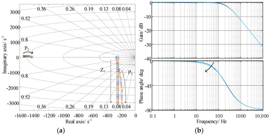
Figure 8.
Pole-zero distribution diagram and Bode plots under . (a) Closed-loop zero-pole distribution diagram. (b) Closed-loop Bode plots.
3.2. Design of Internal Model Current Decoupling Controller in Discrete Domain
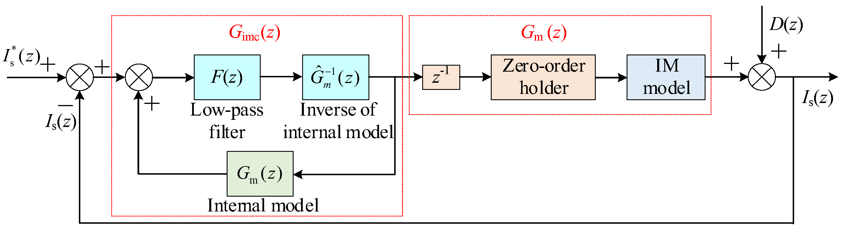
When the switching frequency is low, the current internal model controller should be designed in the discrete domain (z-domain). The z-domain equivalent structure diagram of the internal model control system is shown in Figure 9, where z−1 represents the model of the sampling and control delay, and the zero-order holder represents the model of the inverter.
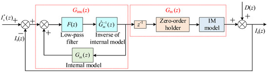
Figure 9.
Equivalent structure diagram of internal model control system in z-domain.
F(z) is used to reduce the high-frequency oscillation; its z-domain transfer function is expressed as follows:
where k is the coefficient of F(z), and Ts is the switching period.
The s-domain transfer function Gzoh(s) of the zero-order holder is expressed as follows:
Considering the sampling delay and zero-order holder, the Gm(s) is discretized, the transfer function of Gm(z) is obtained as follows:
The transfer function of Gimc(z) is derived as follows:
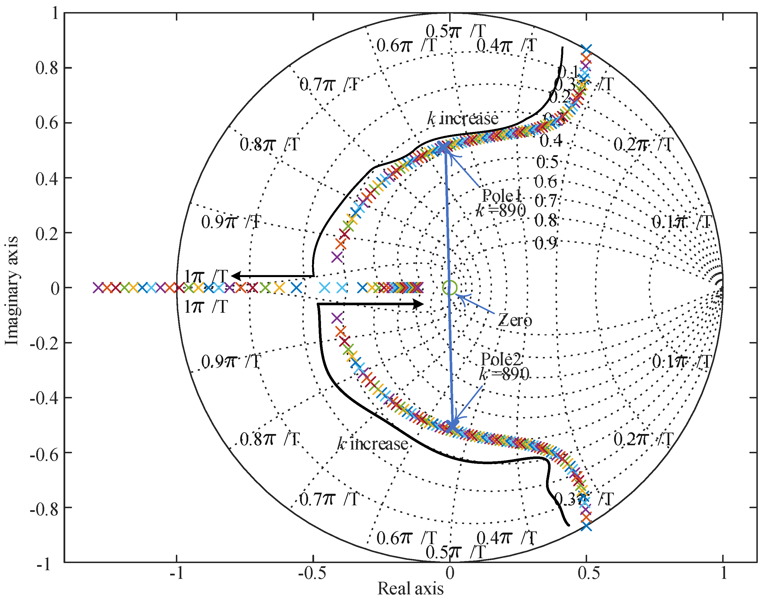
It can be seen that no item in Gclose(z) contains ωe. When k varies within the range of [0, 2000], the zero-pole distribution diagram of the current closed-loop transfer function is shown in Figure 10. There are two poles and one zero, and the zero is located at the center of the unit circle. As k increases, the two conjugate poles move to the left while approaching the real axis. According to the discrete-time control theory, as the distance between the pole and the center of the unit circle decreases, the dynamic response becomes faster. As the z-domain conjugate poles shift to the left, the imaginary part of the corresponding s-domain conjugate poles increases, leading to an increase in oscillations during the dynamic process. In Figure 10, when k is greater than 890, the distance between the pole and the center of the unit circle decreases marginally, so k is determined as 890 in this paper.
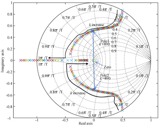
Figure 10.
Migration of poles/zeros of digital control system according to increase in k.
4. Experimental Results
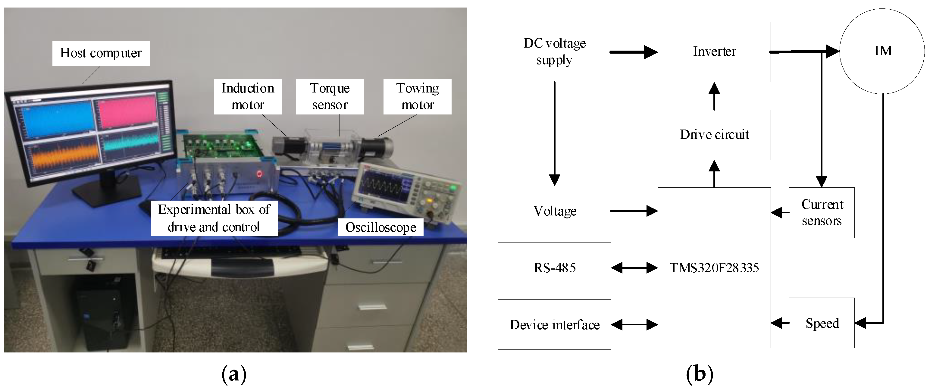
The experimental images and structure diagram used in this paper are shown in Figure 11. The experimental system mainly consists of four parts: an induction motor towing platform, an experimental box of drive and control, a cSPACE upper computer, and related sensors. The parameters of the induction motor have been listed in Table 1. The sensors used in the experimental system mainly include a torque sensor (type: WTQ1050D, bandwidth: 6 kHz, Nanli Measurement and Control Equipment Co., Ltd., Donguan, China), a hall current sensor (type: ACS711ELCTR-25AB-T, Allegro MicroSystems, Worcester, MA, USA), and photoelectric incremental encoders (type: TS5700N8501, Tamagawa, Tokyo, Japan) with a wire count of 2500PPR. The control algorithm is implemented by the digital signal processor (type: TMS320F28335, Texas instruments, Dallas, TX, USA), and the adopted numerical integration algorithm is the forward Euler method. The driving system is mainly composed of six driving chips (type: IRS923STRPBF, Infineon, Munich, Germany). In addition, the experimental box includes a Power module, RS-485 bus, USB to serial port, torque signal amplifier, etc.
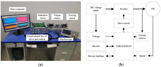
Figure 11.
The experimental setup. (a) Platform overview. (b) Platform block.
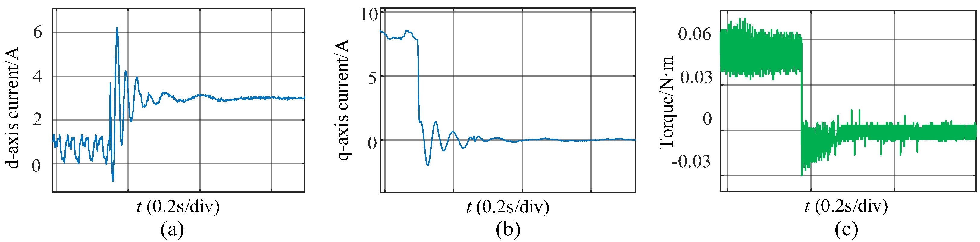
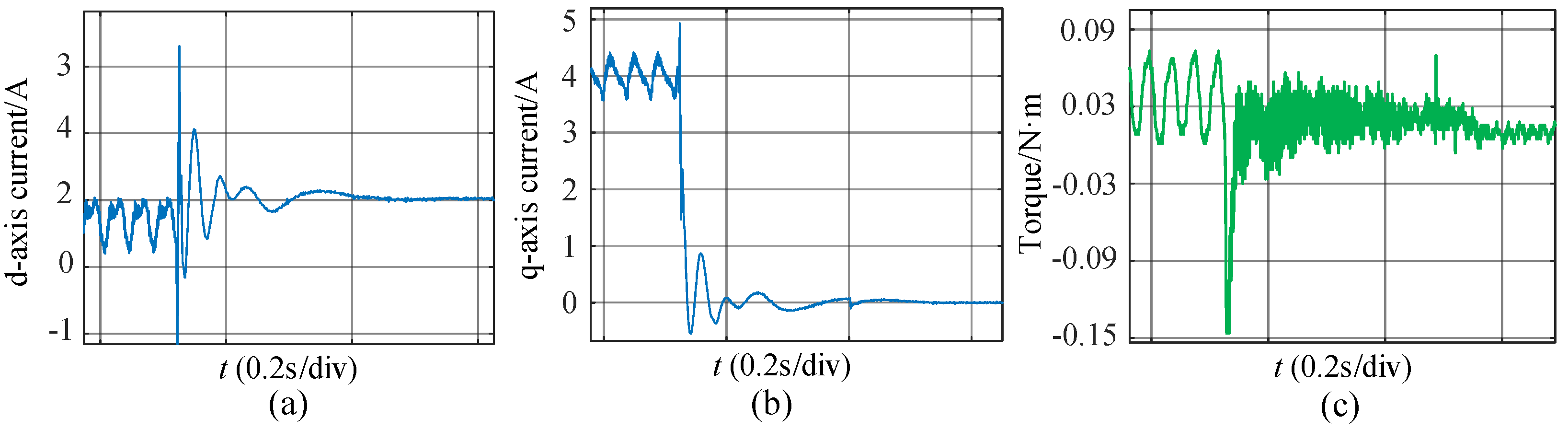
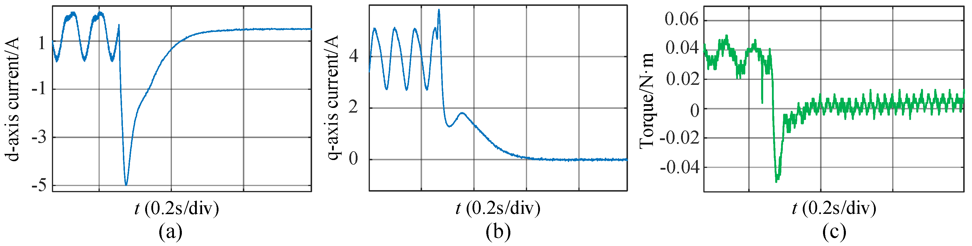
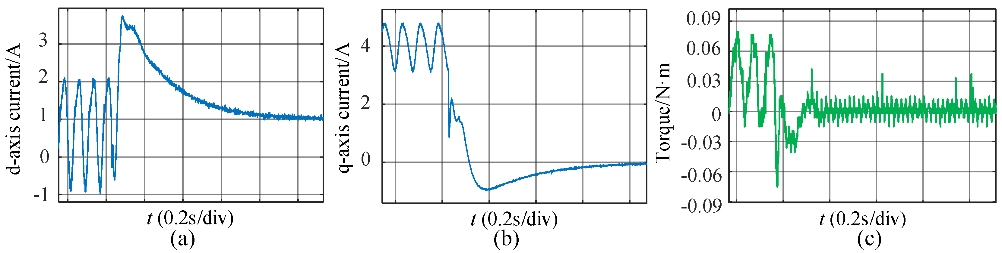
The PWM frequency is set to 15 kHz, the reference of the speed is 2500 rpm, and the IM operates with no load. The references of id and iq are set as 1 A and 8 A, respectively. When the IM operates in a steady state, the references of id and iq are step-changed to 3 A and 0 A at different times. The dynamic experimental waveforms of torque, id and iq, under three different control methods are shown in Figure 12, Figure 13, and Figure 14, respectively.
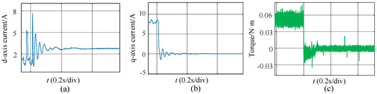
Figure 12.
The dynamic experimental waveforms under PI current controller without decoupling compensation. (a) d-axis current. (b) q-axis current. (c) Electromagnetic torque.

Figure 13.
The dynamic experimental waveforms under PI current controller with the feedforward decoupling. (a) d-axis current. (b) q-axis current. (c) Electromagnetic torque.
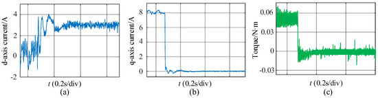
Figure 14.
The dynamic experimental waveforms under the proposed internal model current controller. (a) d-axis current. (b) q-axis current. (c) Electromagnetic torque.
Figure 12 shows the d-axis and q-axis current and torque responses when using a PI current controller without decoupling compensation. From Figure 13a,b, it can be observed that the d-axis and q-axis current exhibit oscillatory decay, with the d-axis current oscillating peak exceeding 7 A and the q-axis current oscillating peak reaching −2 A, which indicates a strong d–q axis cross-coupling. Figure 13 shows the feedforward decoupling dynamic response under the same conditions. Compared with no decoupling shown in Figure 12, the peak value of d-axis current oscillation during feedforward decoupling in Figure 13a has decreased but still exceeds 6 A. The electromagnetic torque of Figure 13c exhibits negative overshoot due to cross-coupling, with a peak overshoot of approximately 0.03 N·m. Figure 14 shows the experimental waveform when using the proposed internal model current controller. Due to the presence of cross-integration terms, it can be observed that the overshoot of the d-axis stator current and q-axis stator current relative to the references are significantly reduced, the peak value of the d-axis stator current oscillation is below 4 A, and the peak value of electromagnetic torque overshoot in Figure 15c is only 0.015 N·m, which is about 50% lower than that with no decoupling and feedforward decoupling.
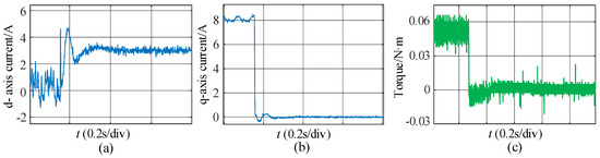
Figure 15.
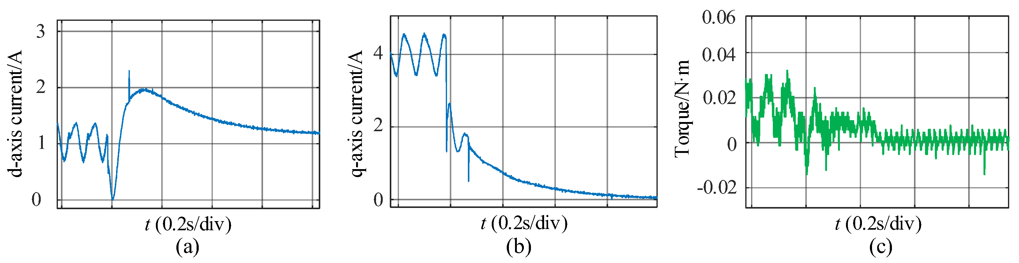
The dynamic experimental waveforms under the proposed internal model current controller when . (a) d-axis current. (b) q-axis current. (c) Electromagnetic torque.
Due to the fact that the motor parameter involved in the cross-decoupling term in the internal model current controller is stator leakage inductance, Figure 15 shows the decoupling effect of the internal model current controller under . Compared to experimental waveforms in Figure 14 without parameter mismatch, the dynamic responses of the d-axis stator current, the q-axis current, and electromagnetic torque have little variation, and the experimental results are consistent with the theoretical analysis. Therefore, the proposed internal model control scheme has the ability to suppress the effects of the stator inductance mismatch.
Next, the effectiveness of the designed internal model current controller in the z-domain will be verified. The switching frequency is reduced to 2 kHz, the reference of the speed is 500 rpm, and the IM operates with no load. The references of id and iq are set as 1 A and 4 A, respectively. When the IM operates at a steady state, the reference of iq is step-changed to 0A. The dynamic experimental waveforms of torque, id and iq, under four different control methods are shown in Figure 16, Figure 17, Figure 18, and Figure 19, respectively.
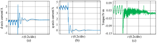
Figure 16.
The dynamic experimental waveforms under the PI current controller with low switching frequency and decoupling compensation. (a) d-axis current. (b) q-axis current. (c) Electromagnetic torque.
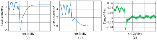
Figure 17.
The dynamic experimental waveforms under the PI current controller with low switching frequency and feedforward decoupling. (a) d-axis current. (b) q-axis current. (c) Electromagnetic torque.
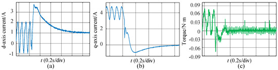
Figure 18.
The dynamic experimental waveforms with low switching frequency under the proposed internal model current decoupling controller in the s-domain. (a) d-axis current. (b) q-axis current. (c) Electromagnetic torque.
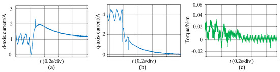
Figure 19.
The dynamic experimental waveforms with low switching frequency under the proposed internal model current decoupling controller in the z-domain. (a) d-axis current. (b) q-axis current. (c) Electromagnetic torque.
Figure 16 shows the d-axis and q-axis current and torque responses when using a PI current controller without decoupling compensation. Compared with Figure 12, due to a low switching frequency, the ripple of the d-axis current increases, and with the sudden change in the q-axis stator current, id exhibits attenuation oscillation. As a result, an overshoot of −0.15 N·m occurs in electromagnetic torque, as shown in Figure 16c. Figure 17 shows the feedforward decoupling dynamic response under the same conditions. Compared with no decoupling shown in Figure 16, the d-axis stator current no longer decays and oscillates, but there is an impulse of −5A. The overshoot of electromagnetic torque is −0.05 N·m, which is less than that of decoupling. Figure 18 shows the dynamic experimental waveforms under the designed internal model current decoupling controller in the s-domain; the overshoot of the d-axis stator current is 3.6 A, and the dynamic performance of the electromagnetic torque is weaker than that of feedforward decoupling, which indicates that the designed internal model current decoupling controller in the s-domain does not have excellent dynamic performance at low switching frequency. Figure 19 shows the dynamic experimental waveforms under the designed internal model current decoupling controller in the z-domain; the overshoot of the d-axis stator current is limited, the electromagnetic torque variation in Figure 19c is smoother, and the overshoot is significantly limited to only −0.01 N·m. Therefore, the theoretical analysis in Part 3.2 of Section 3 is correct.
Then, the steady state under the designed internal model current controller in the z-domain is compared with the traditional PI current controller with feedforward decoupling. The switching frequency is reduced to 2 kHz, the reference of the speed is 1500 rpm, the IM operates with the load of 5 N·m, and the reference of id is set as 5 A. The steady-state waveforms and FFT analysis results are shown in Figure 20 and Figure 21.
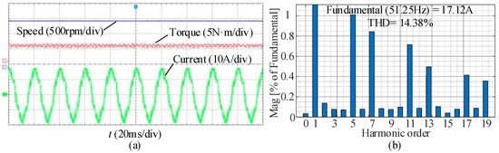
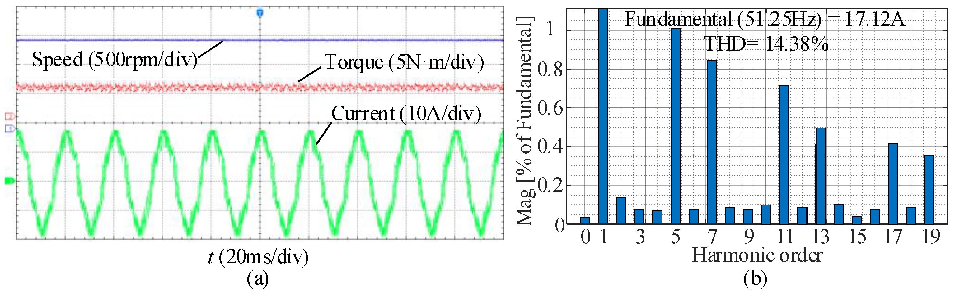
Figure 20.
The steady-state experimental waveforms and FFT analysis results under the traditional PI current controller with feedforward decoupling. (a) Waveforms. (b) FFT analysis results.
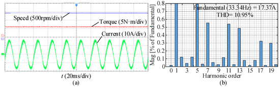
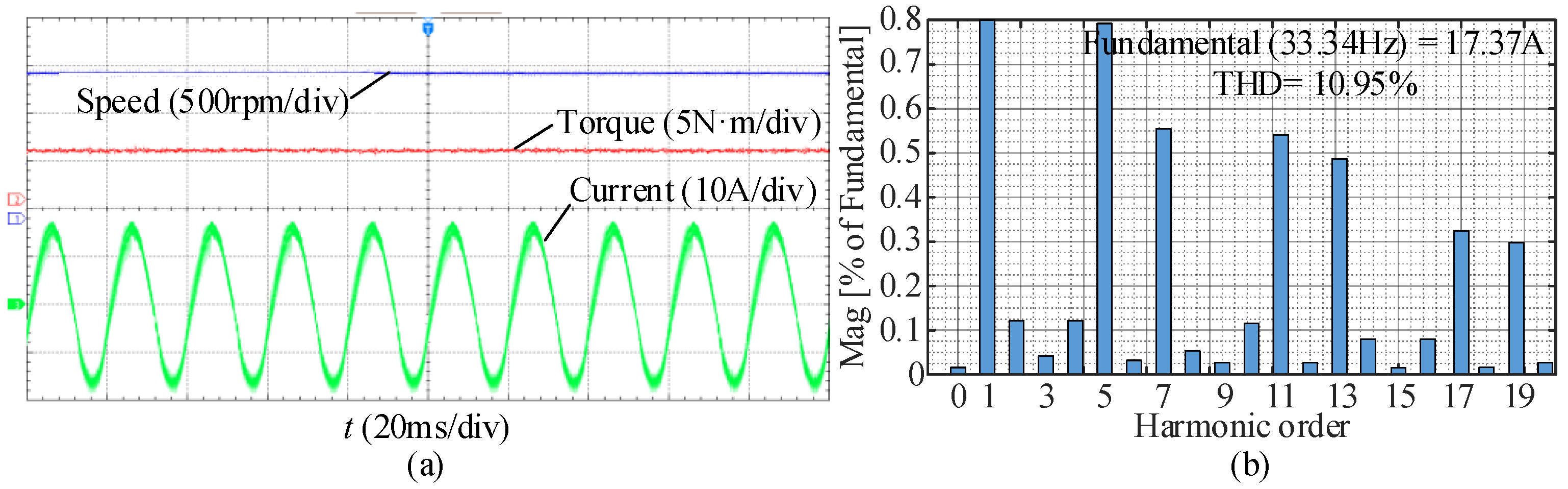
Figure 21.
The steady-state experimental waveforms and FFT analysis results under the proposed internal model current decoupling controller in the z-domain. (a) Waveforms. (b) FFT analysis results.
Since the switching frequency is low, in Figure 20, the ripple of the torque under the traditional PI current controller is great, and the THD of the current is 14.38%. Since the proposed internal model current decoupling controller in the z-domain can compensate for control delay caused by low switching frequency, in Figure 21, the torque ripple and the current harmonic distortion are less than those under the traditional PI current controller, so a better steady-state performance can be obtained by the proposed control method.
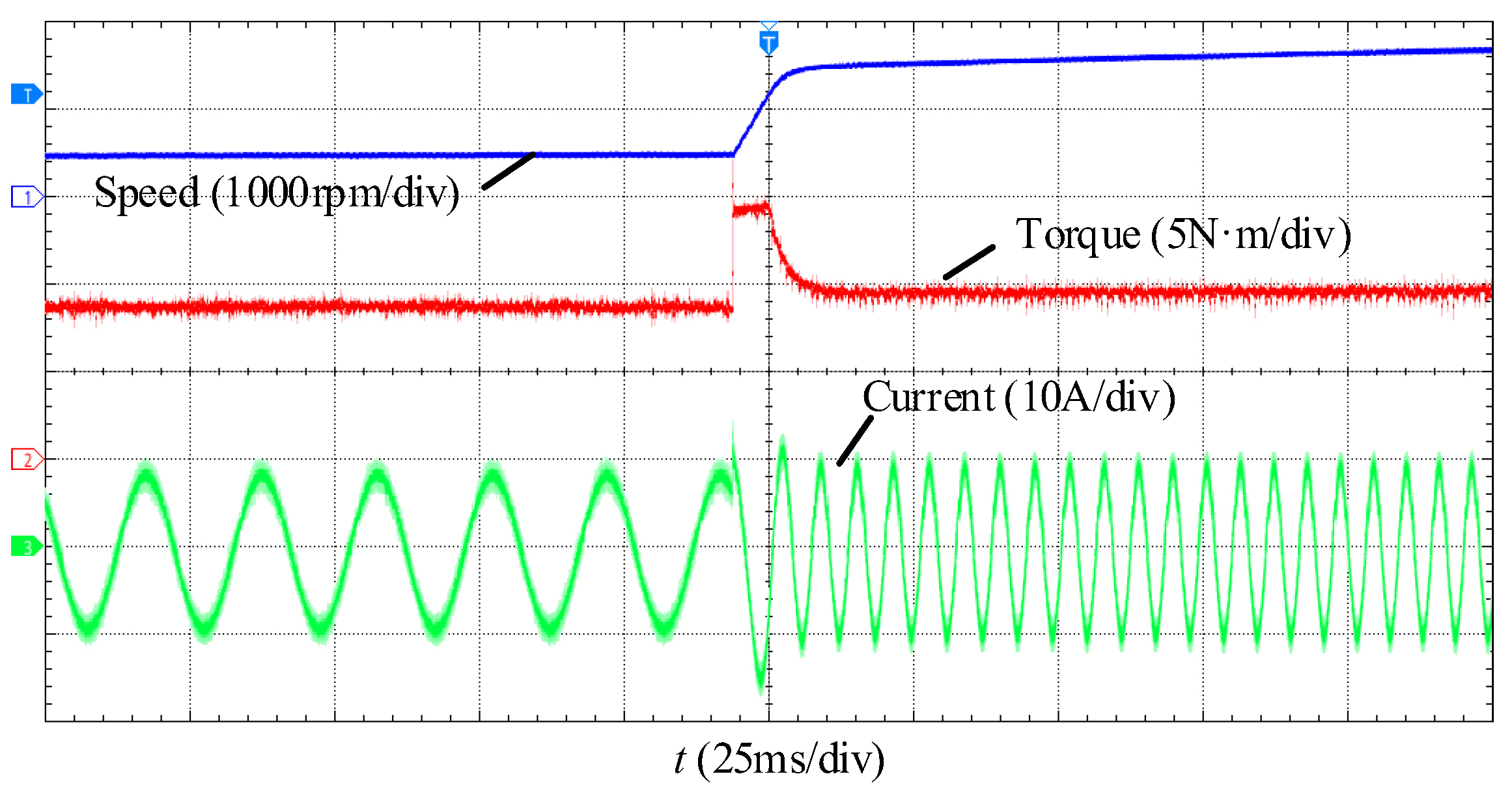
To further verify the effectiveness of the proposed internal model control method under speed increasing, the dynamic experimental waveforms when the speed changes from 400 rpm to 1600 rpm with a load of 8 N·m are shown in Figure 22. The acceleration time is shorter than 15 ms, and no overshoot or oscillation occurs in the dynamic process, which shows that good dynamic performance can be obtained by the proposed internal model control method.
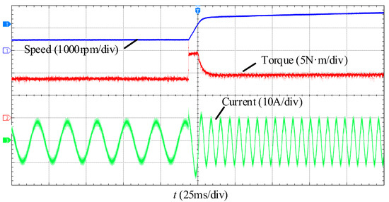
Figure 22.
Dynamic experimental waveforms when the speed changes from 400 rpm to 1600 rpm.
5. Conclusions
This paper proposes an internal model current decoupling control strategy to suppress the stator internal coupling effect; the coupling characteristic of IMs is analyzed, and the design details for the structure and parameters of the internal model controller are presented in continuous and discrete domains, respectively. Finally, its feasibility and effectiveness have been proven by the experimental results, and the following conclusions are formed:
- (1)
- There is a complex pole in the IM mathematical model: as the synchronous speed increases, the imaginary axis component of the complex pole increases, resulting in an increasing oscillation during the dynamic process;
- (2)
- The internal model controller generates a zero at the same position as the complex pole, eliminating the stator’s internal coupling. Meanwhile, it is insensitive to stator leakage inductance;
- (3)
- Considering sampling and control delay, an internal model controller is designed in a discrete domain, the parameter is determined according to the phase of the pole and the distance between the pole and the center of the unit circle. A good dynamic performance can be obtained under the switching frequency of 2 kHz.
Author Contributions
Conceptualization, Q.X. (Qiuyue Xie); Methodology, Q.X. (Qiwei Xu); Validation, Q.X. (Qiwei Xu); Investigation, Y.T.; Data curation, Y.T.; Writing—original draft, Q.X. (Qiuyue Xie) and Y.T.; Writing—review & editing, Q.X. (Qiwei Xu) and T.Y.; Supervision, T.Y.; Project administration, Q.X. (Qiuyue Xie); Funding acquisition, T.Y. All authors have read and agreed to the published version of the manuscript.
Funding
This research was funded by [Hunan Institute of Engineering, National key research and development plan] grant number [2022YFB3403202], [Hunan Institute of Engineering, Department of Education outstanding youth project of Hunan Provincial] grant number [23B0702], [Wenzhou basic scientific research project] grant number [S20240002], [Wenzhou major scientific and technological innovation projects] grant number [ZG2024034] and [Doctoral Research Foundation of Chongqing Industry Polytechnic College] grant number [2022GZYBSZK1-04].
Data Availability Statement
The original contributions presented in the study are included in the article, further inquiries can be directed to the corresponding author.
Conflicts of Interest
The authors declare no conflict of interest.
References
- Liao, W.; Tong, Y.; Huang, S.; Liang, G.; Feng, C.; Wu, X.; Huang, S. A Carrier Self-Synchronization Method for Distributed Control Units in Multithree-Phase Permanent Magnet Synchronous Motor. IEEE Trans. Ind. Electron. 2024, 72, 4353–4363. [Google Scholar] [CrossRef]
- Onsal, M.; Demir, Y.; Aydin, M. Impact of Asymmetric and Symmetric Overhangs on Torque Quality and Axial Magnetic Force Computations in Surface Mounted PM Synchronous Motors. IEEE Trans. Magn. 2021, 58, 8201505. [Google Scholar] [CrossRef]
- Dong, Z.; Song, Z.; Wang, W.; Liu, C. Improved Zero-Sequence Current Hysteresis Control-Based Space Vector Modulation for Open-End Winding PMSM Drives With Common DC Bus. IEEE Trans. Ind. Electron. 2023, 70, 10755–10760. [Google Scholar] [CrossRef]
- Zhang, Y.; Xu, S.; Song, Y.; Qi, W.; Guo, Q.; Li, X.; Kong, L.; Chen, J. Real-Time Global Optimal Energy Management Strategy for Connected PHEVs Based on Traffic Flow Information. IEEE Trans. Intell. Transp. Syst. 2024, 25, 20032–20042. [Google Scholar] [CrossRef]
- Dong, Z.; Huang, R.; Liu, S.; Liu, C. Analysis of Winding-Connection Sequence in Multiphase Series-End Winding Motor Drives for Leg-Current Stress Reduction. IEEE Trans. Ind. Inform. 2025, 21, 1635–1644. [Google Scholar] [CrossRef]
- Arandhakar, S.; Jayaram, N.; Shankar, Y.R.; Gaurav; Kishore, P.S.V.; Halder, S. Emerging Intelligent Bidirectional Charging Strategy Based on Recurrent Neural Network Accosting EMI and Temperature Effects for Electric Vehicle. IEEE Access 2022, 10, 121741–121761. [Google Scholar] [CrossRef]
- Montoya-Acevedo, D.; Gil-González, W.; Montoya, O.D.; Restrepo, C.; González-Castaño, C. Adaptive Speed Control for a DC Motor Using DC/DC Converters: An Inverse Optimal Control Approach. IEEE Access 2024, 12, 154503–154513. [Google Scholar] [CrossRef]
- Xu, Q.; Wang, Y.; Miao, Y.; Zhang, X. A Double Vector Model Predictive Torque Control Method Based on Geometrical Solution for SPMSM Drive in Full Modulation Range. IEEE Trans. Ind. Electron. 2024, 1–11. [Google Scholar] [CrossRef]
- Dong, Z.; Liu, Y.; Zhang, B.; Liu, C. Half Open-End Winding Topology Based Nine-Leg VSI for Asymmetrical Six-Phase PMSM Drives. IEEE Trans. Power Electron. 2023, 38, 11399–11410. [Google Scholar] [CrossRef]
- Zhang, Q.; Fan, Y.; Mao, C. A Gain Design Method for a Linear Extended State Observers to Improve Robustness of Deadbeat Control. IEEE Trans. Energy Convers. 2020, 35, 2231–2239. [Google Scholar] [CrossRef]
- Dong, N.; Li, M.; Chang, X.; Zhang, W.; Yang, H.; Zhao, R. Robust Power Decoupling Based on Feedforward Decoupling and Extended State Observers for Virtual Synchronous Generator in Weak Grid. IEEE J. Emerg. Sel. Top. Power Electron. 2023, 11, 576–587. [Google Scholar] [CrossRef]
- Song, P.; Liu, Y.; Liu, T.; Wang, H.; Wang, L. A Novel Suppression Method for Low-Order Harmonics Causing Resonance of Induction Motor. Machines 2022, 10, 1206. [Google Scholar] [CrossRef]
- Liu, X.; Hou, M.; Wang, X. Complex Vector Analysis and 2DOF Internal Model Decoupling Control for Toroidal Motor. IEEE Trans. Appl. Supercond. 2021, 31, 1–5. [Google Scholar] [CrossRef]
- Sun, X.; Wu, C.; Wang, J. Adaptive Compensation Flux Observer of Permanent Magnet Synchronous Motors at Low Carrier Ratio. IEEE Trans. Energy Convers. 2021, 36, 2747–2760. [Google Scholar] [CrossRef]
- Wu, X.; Zhu, Z.-Q.; Freire, N.M.A. High Frequency Signal Injection Sensorless Control of Finite-Control-Set Model Predictive Control With Deadbeat Solution. IEEE Trans. Ind. Appl. 2022, 58, 3685–3695. [Google Scholar] [CrossRef]
- Wang, F.; He, L. FPGA-Based Predictive Speed Control for PMSM System Using Integral Sliding-Mode Disturbance Observer. IEEE Trans. Ind. Electron. 2021, 68, 972–981. [Google Scholar] [CrossRef]
- Wang, S.; Wang, H.; Tang, C.; Wang, L.; Zhu, Y.; Liu, H.; Wang, S. Sensorless Control Strategy for Permanent Magnet Synchronous Motor Based on Adaptive Non-Singular Fast Terminal Sliding Mode Observer. IEEE Trans. Appl. Supercond. 2024, 34, 5208905. [Google Scholar] [CrossRef]
- Zhang, X.; Xu, Q.; Miao, Y.; Wu, X.; Wang, Y.; Yi, L. An Improved Generalized Extended State Observer for Current Harmonic Compensation in Dual Three-Phase PMSMs. IEEE Trans. Power Electron. 2025, 40, 7136–7149. [Google Scholar] [CrossRef]
- Novak, M.; Xie, H.; Dragicevic, T.; Wang, F.; Rodriguez, J.; Blaabjerg, F. Optimal Cost Function Parameter Design in Predictive Torque Control (PTC) Using Artificial Neural Networks (ANN). IEEE Trans. Ind. Electron. 2021, 68, 7309–7319. [Google Scholar] [CrossRef]
- Kim, D.-J.; Hong, D.-K.; Choi, J.-H.; Chun, Y.-D.; Woo, B.-C.; Koo, D.-H. An Analytical Approach for a High Speed and High Efficiency Induction Motor Considering Magnetic and Mechanical Problems. IEEE Trans. Magn. 2013, 49, 2319–2322. [Google Scholar] [CrossRef]
- Miao, Y.; Liao, W.; Huang, S.; Liu, P.; Wu, X.; Song, P.; Li, G. DC-Link Current Minimization Scheme for IM Drive System Fed by Bidirectional DC Chopper-Based CSI. IEEE Trans. Transp. Electrif. 2023, 9, 2839–2850. [Google Scholar] [CrossRef]


Disclaimer/Publisher’s Note: The statements, opinions and data contained in all publications are solely those of the individual author(s) and contributor(s) and not of MDPI and/or the editor(s). MDPI and/or the editor(s) disclaim responsibility for any injury to people or property resulting from any ideas, methods, instructions or products referred to in the content. |
© 2025 by the authors. Licensee MDPI, Basel, Switzerland. This article is an open access article distributed under the terms and conditions of the Creative Commons Attribution (CC BY) license (https://creativecommons.org/licenses/by/4.0/).