


Abstract
As the share of wind and photovoltaic generation in power systems increases, renewable generation and storage are increasingly participating in bidding in electricity markets. However, fluctuations in renewable output, uncertain market prices, and intertemporal coupling in storage operation complicate bidding and increase operating risks. This study develops an electricity energy market simulation framework covering medium- and long-term trading and spot-market trading. The Win or Learn Fast policy hill-climbing (WoLF-PHC) algorithm is used to model multi-agent bidding, accounting for contract settlement, deviation assessment, operating characteristics of conventional units, and constraints on the storage state of charge. Joint renewable-storage operation and independent participation are compared in terms of policy convergence, participant operating profit, consumer procurement cost, renewable utilization, and storage operation. The case study supports the effectiveness of the framework and shows that market participants can develop stable bidding policies. Compared with independent participation, joint operation coordinates energy internally between renewable plants and storage facilities, improving system operating performance while reducing consumer procurement costs and promoting renewable utilization.
1. Introduction
Global decarbonization and the development of modern power systems continue to drive growth in installed wind and photovoltaic (PV) capacity. The generation mix is shifting from controllable fossil-fuel resources toward coordinated operation of diverse energy resources [1,2]. Meanwhile, electricity-market reform in China has expanded trading from medium- and long-term contracts to spot and ancillary-service markets, strengthening the role of price signals in resource allocation. Renewable producers have consequently evolved from passive recipients of guaranteed purchases into market participants that compete and bear responsibility for deviations. Energy storage has also become integral to market operation and value formation because it can shift energy over time and respond rapidly [3,4]. Effective coordination between contracts and real-time markets is therefore essential for balancing short-term operating efficiency, risk management, and long-term investment incentives [5].
Renewable output is stochastic and variable, and forecast errors create differences between scheduled and actual generation. These differences can trigger imbalance settlement, deviation penalties, and revenue losses. Supply–demand conditions, strategic behavior, and policy changes further amplify price uncertainty [6,7]. As variable generation increases, systems require more balancing of resources and operating flexibility, making balancing markets increasingly important [8]. Resource endowments, weather, and electricity prices also cause revenue risk for renewable producers to span multiple time scales [9]. Storage can mitigate renewable deviations through charging and discharging. However, its operation is constrained by power ratings, state of charge (SOC), conversion efficiency, cycle life, and intertemporal energy balance. Changing market conditions also require a trade-off between flexibility and operating cost [10]. Coordinating forecast errors, price risk, physical constraints, and strategic behavior under incomplete information is central to participant profitability and system efficiency [11].
Existing bidding methods address these challenges through mathematical optimization, game-theoretic analysis, price forecasting, and intelligent decision-making. Stochastic programming represents output and price uncertainty through scenarios; robust optimization controls adverse-scenario risk through uncertainty sets; and bilevel programming captures the nested relationship between participant bids and market clearing [12,13,14]. Although mathematically explicit, these methods commonly require assumed probability distributions, complete information, or an exact market model, and may suffer from scenario proliferation and non-convexity. Traditional electricity-market studies have also examined market power and its influence on strategic bidding [15]. Cooperative, non-cooperative, Stackelberg, and evolutionary games provide systematic tools for representing strategic interactions among participants [13,14,16]. Price forecasts supply external information for bidding and have progressed from statistical and machine-learning models to deep learning, with increasing emphasis on common datasets, benchmarks, and evaluation protocols [17,18,19,20]. Forecast accuracy, however, does not necessarily yield optimal bids. Single-agent reinforcement learning updates policies directly from environmental feedback but generally treats other participants as part of the environment, inadequately representing the non-stationarity created when multiple learning agents act simultaneously [21,22].
Electricity markets inherently involve participants with different objectives, information, and constraints, making multi-agent methods well suited to their distributed decision structure. Early studies modeled generating units, distributed resources, storage, and consumers as interacting autonomous agents and used distributed algorithms for task allocation, information exchange, and market coordination [23]. Agent-based market simulations further showed that learning rules and risk preferences alter competition and market outcomes, so bidding models must explicitly represent interactions among participants [24]. Multi-agent reinforcement learning formalizes states, actions, rewards, and inter-agent coupling within a Markov game, enabling participants to update their policies from local observations, clearing outcomes, and profit feedback. Centralized training with decentralized execution can use joint information during training to improve stability while relying only on locally available information during actual decisions. This provides a general framework for partial observability, credit assignment, growth in the joint action space, and equilibrium selection [25].
Multi-agent research on strategic generator bidding initially focused on competitive equilibria and policy learning in day-ahead markets. Du et al. (2021) modeled generators as learning agents and used multi-agent deterministic policy gradients to approximate day-ahead Nash equilibrium under partial observability [26]. Their results supported the feasibility of interactive learning for strategic bidding. Subsequent work developed participant-specific bidding frameworks whose state spaces include historical clearing information, market conditions, and rival behavior, thereby producing more adaptive bid policies [27]. To address market-rule changes and limited training samples, Wu et al. (2022) transferred policy knowledge from a source market to a target market [28]. This approach shortened training and improved decisions under new rules. Collectively, these studies show that multi-agent methods can incorporate competitors’ evolving strategies into continual learning rather than treating other participants as a fixed environment.
As renewable and storage participation has deepened, multi-agent bidding research has expanded beyond competition among homogeneous generators. It now covers coordinated operation across renewable resources, storage systems, and multiple markets. Studies of storage participation in energy and frequency-regulation markets model wind power, conventional generation, and storage as distinct agents. Their joint state space represents charging and discharging power, regulation capacity, and intertemporal state of charge, thereby capturing how storage allocates flexibility among services [10]. Multi-agent models for joint wind-thermal-storage bidding account for renewable deviations, conventional-unit costs, and rapid storage response. These models coordinate competition across energy and regulation markets [29]. Two-stage models also combine day-ahead price forecasts informed by carbon, green-certificate, and fuel prices with multi-agent bidding decisions. This approach links the behavior of wind, hydropower, thermal generation, and purchasers directly to market objectives [30].
Unlike metaheuristic global optimization algorithms, such as the Musical Chairs Algorithm (MCA) and the Star-Nosed Mole Optimizer (SNMO) [31,32], multi-agent methods such as the Win or Learn Fast policy hill-climbing (WoLF-PHC) algorithm do not directly solve optimization problems for storage sizing. Instead, they evaluate the market returns of renewable plants at a given storage capacity by analyzing bidding decisions and profits. In retail markets, multi-agent reinforcement learning can combine consumers’ price perceptions with demand response to represent bilateral bidding between retailers and consumers [33]. Evolutionary games combined with Q-learning and swarm intelligence can describe limited information and strategy evolution in end-user demand-response bids [34]. In coupled electricity, carbon, and green-certificate markets, agents can adapt their transactions simultaneously, revealing how price linkages and policy mechanisms affect profits and energy choices [35]. Continuous double-auction studies place agents on both the supply and demand sides to simulate bilateral bidding and network-constrained clearing [36]. For decentralized renewable-energy trading, evolutionary-game studies further reveal dynamic strategy adjustment as the competitive environment changes [37].
Overall, multi-agent algorithms can represent bidding competition among renewable generators, storage systems, thermal generators, hydropower generators, and consumers in a common market. They update bids iteratively from repeated clearing outcomes. Each generator selects a piecewise bid curve, and market clearing determines its awarded quantity and the market-clearing price (MCP). The generator then calculates its return from revenue from electricity sales, generation cost, contract settlement, and deviation charges. Higher-return bids consequently become more likely to be selected again. Two gaps remain in simulation-based analyses of electricity energy market bidding decisions. The first concerns a closed-loop framework linking bidding, clearing, operation, and settlement, including medium- and long-term contract settlement through contracts for difference (CfDs), K-recovery, and deviation assessment. The second concerns the analysis of bidding strategies and returns within a unified electricity energy market simulation framework.
To address these gaps, this study develops an electricity energy market simulation framework covering medium- and long-term and spot markets. It investigates strategic bidding and operational performance when renewable generation and storage participate across multiple market time scales. The main contributions are as follows:
- (1)
- This study develops a coordinated electricity energy market simulation framework linking medium- and long-term trading with spot-market operation. Monthly and weekly trading are integrated with day-ahead, intraday, and real-time stages. Decomposition of contract energy, CfD settlement, real-time deviation assessment, and the periodic K-recovery mechanism link contract performance across these markets. Thermal-unit start-up, shutdown, and ramping limits, uncertainty in renewable output, and storage state-of-charge constraints are incorporated into a closed loop of bidding, clearing, operation, and settlement. A heterogeneous WoLF-PHC multi-agent bidding model represents thermal-power, hydropower, wind-storage, photovoltaic-storage, and demand-side participants as independent agents. Action spaces are defined for non-decreasing piecewise bids and load adjustments, and rewards combine spot-market returns, CfD settlement, K-recovery, deviation smoothing, and storage value. WoLF-PHC adjusts policies slowly when winning and quickly when losing, allowing participants to adapt their bids competitively and linking market simulation with bidding decisions.
- (2)
- This study establishes a multidimensional evaluation framework covering algorithmic, electricity energy market, and physical operating performance. Under identical input data, medium- and long-term strategies, and training conditions, it compares joint renewable-storage operation and independent participation. Evaluation covers training convergence, operating profit, consumer procurement cost, contract performance, renewable curtailment, and storage operation. The case study shows that joint operation can increase profit and reduce curtailment by coordinating renewable output with storage charging and discharging, balancing system economics and consumer cost.
The remainder of this study is organized as follows. Section 2 introduces the multi-timescale electricity-market structure and formulates bidding and clearing models for generation, medium- and long-term trading, and real-time trading. Section 3 develops the WoLF-PHC multi-agent bidding model, including the state spaces, action spaces, reward functions, and solution procedure for demand- and generation-side agents. Section 4 evaluates training stability, economic performance, and renewable integration through a case study, participation-mode comparisons, and storage energy–power sensitivity analyses. Section 5 summarizes the main findings, limitations, and directions for future work.
2. Market Structure and Market Participant Bidding Model
Modern electricity energy markets span medium- and long-term trading and day-ahead, intraday, and real-time operation. Medium- and long-term markets cover annual, monthly, and weekly transactions; forward contracts are concluded through bilateral negotiation or centralized bidding to lock in energy and prices, mitigate exposure risk, and stabilize generators’ baseline revenues. In the day-ahead spot market, generators submit piecewise price–quantity bids, and joint security-constrained unit commitment and security-constrained economic dispatch determine generation schedules and locational marginal prices. The intraday market updates day-ahead deviations on a rolling basis, while the real-time market performs final balancing every 15 (or 5) min. Real-time price fluctuations reflect system scarcity and reward flexible resources. These four layers provide the broader market context. To focus on electricity energy market simulation using artificial intelligence, the proposed model adopts a basic centralized pool framework without transmission constraints [38]. Clearing is represented as a uniform-price auction, allowing analysis of participants’ intertemporal bidding strategies and coordinated returns.
2.1. Analysis of Market Structure
The electricity energy market architecture developed in this study comprises monthly and weekly medium- and long-term markets, day-ahead and intraday spot markets, and a real-time market operating at 15 min intervals. This architecture supports analysis of electricity-market participants’ bidding decisions across multiple time scales.
The medium- and long-term market is centered on monthly contracts, supplemented by weekly transactions. Generators and consumers enter financially settled energy contracts through centralized bidding, with a one-month contract period. This market layer locks in baseline prices and supply for most electricity, mitigates spot-price risk, and stabilizes expected generator revenue. Medium- and long-term contracts typically cover 70–90% of total consumer demand.
The day-ahead market uses next-day load and renewable-output forecasts. Participants submit hourly bids, which are mapped to 96 15 min intervals for joint clearing to determine awarded energy, prices, and baseline operating schedules. Forecast renewable output enters the agent state and informs bidding and scheduled delivery. Storage schedules account for SOC and charging and discharging constraints across intervals. Day-ahead bid prices and bid-block capacity boundaries are frozen at gate closure.
At each hour, the intraday stage updates the remaining operating schedule using revised load and renewable-output forecasts. Participants select available capacity and charging or discharging intentions according to updated forecasts and actual equipment states. These decisions adjust the day-ahead schedule within physical limits and provide dispatchable limits and reference values for terminal energy for real-time execution. Intraday operation neither resubmits prices nor introduces a separate energy-settlement layer.
The real-time market performs rolling optimization at 15 min intervals using ultra-short-term load and renewable-output forecasts and actual unit operating states. Actual output is revealed after action selection and enters feedback rebalancing as the available power for the current interval. Physical clearing and storage charging and discharging address forecast errors. Remaining surplus energy is counted as curtailment, while delivery below the published real-time schedule is assessed as a shortfall. Revenues and penalties enter agent rewards, allowing policies to learn trade-offs among forecast errors, storage states, and market prices.
Contract-energy decomposition and deviation settlement couple the two market layers. The market operator decomposes medium- and long-term contract energy progressively into 15 min intervals, producing a reference contract quantity (MWh) for each participant and interval. Deviation settlement compares real-time cleared output with this reference quantity and applies a prescribed penalty coefficient to the deviation. This mechanism encourages truthful contract declarations and contract performance.
Renewable-output uncertainty is represented using separate forecast and actual-output series. Forecast output enters the agent state and informs bidding and scheduled delivery, whereas actual output sets the real-time availability limit for clearing and settlement. Storage charging and discharging first balance the forecast error within each plant; remaining surplus energy is treated as renewable curtailment, and delivery shortfalls are included in deviation assessment. The resulting revenue and penalties enter the agent reward, allowing the bidding policy to learn the trade-off among forecast error, storage state, and market price.
To constrain favorable price-difference gains arising from contract deviations, this study introduces a periodic K-recovery mechanism based on the 2024 continuous trial-operation plan for the southern Hebei electricity spot market [39]. The plan was issued by the Hebei Provincial Development and Reform Commission and specifies allowable-range parameters of 90 and 110 and an adjustment factor of 1.05. The simulation adopts this regulatory approach and these parameter values, defines performance as actual energy divided by contract energy, and adapts the accumulation window. This study defines one cycle as 24 h, or 96 15 min intervals, and calculates the performance rate as cumulative actual settled energy divided by cumulative contract energy. The allowable band is 90–110%. When the rate is below 90% and the contract price exceeds the cycle-average real-time price, the favorable price-difference revenue associated with the under-delivered energy is recovered using a multiplier of 1.05. When the rate exceeds 110% and the cycle-average real-time price exceeds the contract price, excess-contract revenue is recovered using the same multiplier. No recovery is applied when performance remains within the band or the price difference is unfavorable. During training, the interval increment in cumulative K-recovery amount provides feedback; final settlement uses the cumulative K-recovery amount at the end of the cycle.
This multi-timescale architecture coordinates medium- and long-term risk hedging with short-term flexibility through market organization and economic signals. It is particularly suitable for power systems with high shares of renewable generation. The resulting multi-timescale electricity energy market architecture is illustrated in Figure 1.
Figure 1.
Electricity energy market architecture.
2.2. Market Participant Bidding Model
The participant bidding models represent the decisions and profit objectives of each actor across the market layers. First, generation-side units submit piecewise bids to maximize profit. The centralized bidding and marginal-clearing model for the medium- and long-term market then determines energy contracts. Finally, economic dispatch subject to unit operating constraints is introduced in the day-ahead, intraday, and real-time stages to determine schedules and actual output that maintain system balance.
2.2.1. Generation-Side Unit Bidding Model
Generation-side participants include thermal, hydropower, wind, photovoltaic, and storage units. Each unit bids to maximize its own profit, and the generic objective function is expressed as follows:
where is the net revenue of generating unit i, is its energy-market revenue, and is its cost.
Generation cost is a primary determinant of generation-side bidding. Because cost structures differ substantially across technologies, this section formulates representative cost models for thermal power, hydropower, and renewable plants equipped with storage.
- (1)
- Thermal unit:
- (2)
- Hydropower unit:
Only fixed operation and maintenance costs are considered for hydropower. Subscript h denotes a hydropower unit; t and t + 1 denote consecutive dispatch intervals. The interval duration is Δt (h), and T denotes the end of the complete scheduling horizon. To represent intertemporal water-use constraints, effective head and unit efficiency are approximated as constant over the horizon. An equivalent conversion coefficient links power output to turbine flow, subject to the following water balance:
Here, Ch,t and Ch,tfix are interval generation cost and fixed operation and maintenance cost (CNY), respectively. Ph,t is hydropower output (MW), and κh is the equivalent conversion coefficient [MW/(m3/s)]. Vh,t is reservoir volume at the interval start (m3), bounded by Vhmin and Vhmax. Ih,t, qh,t, and sh,t denote inflow, turbine flow, and spillage (m3/s), respectively; qhmax is the maximum turbine flow. Vhini and Vhtar denote initial volume and the minimum terminal reserve. The factor 3600 converts hours to seconds. Initial volume and terminal reserve jointly limit water available for generation; intraday and real-time optimization inherit actual reservoir volume.
- (3)
- Renewable plant (wind or photovoltaic generation plus storage):
Charging cost : when storage charges at power for duration , the charged energy is (MWh). Charging cost includes the variable storage-use cost and the energy-loss cost caused by charging inefficiency:
where
is the variable operating cost of the energy-storage system (CNY/MWh), including depreciation, operation, and maintenance costs; is the charging efficiency (), defined as the ratio of energy stored in the battery to charging input energy; is the market electricity price during charging (CNY/MWh); this term represents the additional procurement cost caused by charging losses; is the charging energy loss (MWh).
The charging-cost function can therefore be written as:
where is the energy effectively stored in the battery.
Discharging cost : when storage discharges at power for duration , the delivered energy is . Because the discharging efficiency is , the battery must release (MWh). The discharging cost comprises the variable storage-use cost and the cost associated with discharge losses:
where is the market electricity price during discharge (CNY/MWh), and is the energy loss during discharge (MWh).
2.2.2. Medium- and Long-Term Market Clearing Model
The medium- and long-term market primarily trades energy contracts through centralized bidding and marginal clearing. The monthly and weekly markets are modeled as one-sided procurement auctions. Each generator submits a three-block supply bid, while consumer demand is fixed. The clearing objective minimizes the sum of procurement cost and the load-shedding slack penalty:
Objective function:
where is the set of generators, is the set of consumers; is generator j’s submitted bid (CNY/MWh); is its cleared contract energy (MWh); is the load-shedding penalty coefficient; and is the load-shedding slack variable.
Constraints:
- (1)
- Energy-balance constraint:
- (2)
- Bid-block quantity constraint: the awarded quantity in each bid block cannot exceed the declared capacity of that block.
- (3)
- Total-energy constraint: each participant’s total cleared contract energy cannot exceed its declared quantity limit.
- (4)
- Clearing price: under the single-node uniform marginal-clearing mechanism, the market-clearing price (MCP) is the dual variable of the energy-balance constraint. It represents the incremental optimal procurement cost associated with a 1-MWh increase in market demand. When supply is sufficient and the shortage slack variable is zero, the MCP equals the price of the marginal accepted bid block. When the declared supply is insufficient and the shortage slack variable is positive, the MCP is set by the shortage-penalty price.
2.2.3. Day-Ahead Market Clearing Model
The medium- and long-term stage is denoted by LT; DA, ID, and RT denote day-ahead, intraday, and real-time stages, respectively. Day-ahead clearing uses next-day load and renewable-output forecasts and maps participants’ frozen hourly piecewise bids to 96 15 min intervals. It jointly determines unit commitment, awarded output, and storage charging and discharging schedules. Decomposed contract energy serves as the settlement position. Clearing minimizes bid cost, thermal minimum-output operating and start-up/shutdown costs, storage-use cost, and supply-demand slack penalties.
Objective function: superscript s denotes a spot-market stage, taking DA, ID, or RT. JDA is the full-day objective (CNY), and TDA contains all 96 next-day dispatch intervals. The interval objective and its cost components are defined consistently across stages:
The terms A, B, and C are the rates of bid cost, thermal minimum-output operating cost, and associated storage-use cost (CNY/h), respectively. S is interval start-up/shutdown cost (CNY), and L is measured in CNY. G denotes generators; Gth denotes thermal units, and K denotes storage associated with renewable plants. Indices j, g, k, and b denote generators, thermal units, storage-owning plants, and bid blocks, respectively. The bid-hour mapping h(t) is distinct from the hydropower-unit index h. The frozen block price ρj,β,h(t) is in CNY/MWh, and the awarded block output P is in MW. Thermal bid blocks represent increments above minimum technical output. Bg is minimum-output operating cost (CNY/h); u, y, and z are binary online, start-up, and shutdown variables. Cgstart and Cgstop are event costs (CNY). Variables l and x represent supply shortage and forced system surplus (MW), with penalties πshort and πexcess (CNY/MWh). Here, Δt = 0.25 h. Shared constraints below omit stage superscripts and retain these definitions.
Constraints:
- (1)
- System power balance:
Here, Pj,t denotes thermal or hydropower generation, or net renewable-plant delivery (MW), and Dt is the corresponding stage’s load forecast (MW). Associated storage charging is deducted from plant net delivery and is not added again to system load.
- (2)
- Bid-block output and declared-capacity constraints:
Here, is declared block capacity (MW). Thermal blocks represent increments above minimum output; other participants’ blocks represent delivery capacity. Pjmin is minimum thermal output (MW). The set difference G\Gth contains all non-thermal generators.
- (3)
- Unit-output and water-volume limits:
Here, Pgmax and Phmax are rated thermal and hydropower output limits (MW), respectively. Other symbols retain their definitions and are distinguished by unit indices. Thermal output depends on commitment status; hydropower also satisfies Equations (3)–(6).
- (4)
- Ramping between consecutive intervals:
Superscripts up and down denote upward and downward changes. Rgup, Rgdown, Rhup, and Rhdown are nonnegative thermal and hydropower ramp rates (MW/h). Sgup and Sgdown are allowable thermal start-up and shutdown power changes (MW). The first interval inherits actual output and commitment from the preceding interval. Start-up and shutdown allowances are treated separately from normal online ramping.
- (5)
- Thermal commitment logic and minimum up/down times:
Here, Ug and Dg are the minimum up and down times divided by Δt and rounded upward to interval counts. The summation index r denotes an interval, rather than the rolling origin used later. Known start-up/shutdown histories supply states preceding the scheduling origin. Units whose initial continuous online or offline duration is insufficient retain their original status for the remaining mandatory intervals.
- (6)
- Associated storage and renewable-plant constraints:
Storage energy is updated by adding efficiently stored charging energy and subtracting discharge energy adjusted for discharge efficiency. SOC is stored energy divided by rated energy capacity and is expressed as a ratio or percentage. SOCmin and SOCmax are its bounds; Pchmax and Pdismax are charging and discharging limits (MW). The binary variable v permits charging when equal to 1 and discharging when equal to 0. RE denotes forecast available renewable power, with a hat indicating a forecast. Pcurt denotes ordinary curtailment, and Pgrid,max is the plant grid-delivery limit, all in MW. Associated storage charges are only from its own renewable plant, cannot purchase grid electricity, and cannot charge and discharge simultaneously.
- (7)
- Day-ahead initial and terminal storage conditions:
Here, Ekini is the initial storage energy at the start of the complete operating day (MWh). Equal initial and terminal energy prevents day-ahead profit from being obtained by depleting inventory. Clearing determines day-ahead energy awards, commitment, and intertemporal energy schedules. With integer decisions fixed, day-ahead prices are derived from power-balance dual values and adjusted by Δt. Supply–demand slack triggers a fallback rule based on accepted bids.
2.2.4. Intraday Market Clearing Model
At each hour, intraday operation reoptimizes all remaining intervals through day-end using updated load and renewable-output forecasts. Frozen day-ahead bids remain in force, without separate intraday energy settlement. The resulting physical adjustment schedule provides dispatchable-power limits and storage-energy references for real-time operation.
Objective function:
Here, τ is the current rolling origin, and TID(τ) contains all remaining dispatch intervals before day-end. JID(τ) is the intraday objective (CNY). Interval costs follow Equation (17), with updated forecasts and initial states. The auxiliary variable dID bounds absolute terminal-energy deviation from the storage target (MWh); μk is a positive penalty coefficient (CNY/MWh).
Constraints: intraday clearing inherits power balance, bid-capacity, unit-output, ramping, commitment, and storage constraints in Equations (21)–(33), using updated forecasts. Hydropower inherits actual reservoir volume under Equations (3)–(6). At the rolling origin, executed states replace day-ahead forecast states:
Superscript actual denotes executed states. Ek,τactual and Vh,τactual are actual storage energy and reservoir volume at the rolling origin; Pj,τ−1actual is preceding actual output. Thermal commitment and continuous online/offline durations are also inherited. Subsequent commitment may be adjusted within physical limits, with day-ahead commitment serving as a reference.
The strict day-ahead terminal-energy equality in Equation (34) is replaced during rolling optimization by:
Here, Ektar is the full-day terminal-energy target (MWh), equal to initial day-ahead energy. Equation (37) bounds the auxiliary variable below by the absolute energy difference. Its positive penalty coefficient makes it equal that difference at optimality. This soft terminal target encourages inventory recovery. Charging and discharging are additionally limited by dispatchable fractions selected in the current operating decision:
Here, αchID and αdisID are selected charging and discharging fractions, both dimensionless and between 0 and 1. Thermal operating decisions limit dispatchable increments above minimum technical output; hydropower decisions limit dispatchable output. These limits must accommodate actual initial output and downward-ramping capability. Intraday schedules do not change frozen day-ahead financial positions.
2.2.5. Real-Time Market Clearing Model
Real-time operation optimizes a rolling window at 15 min execution intervals using ultra-short-term forecasts and current equipment states, executing only the first interval. Actual load and renewable output are revealed after operating-action selection. Feedback balancing under the same physical constraints then determines actual delivered energy. Frozen bids remain in force, and intraday decisions additionally constrain dispatchable power.
Objective function:
Here, JRT(τ) is the real-time objective (CNY), and TRT(τ) contains intervals in the current rolling window. The auxiliary variable dRT bounds absolute terminal-energy deviation from the intraday reference (MWh). Other symbols and cost components retain their definitions. Real-time operation uses Equations (21)–(33), initialized with the latest actual states as in Equation (36). After action selection, actual values replace load and renewable forecasts for the first interval; subsequent intervals retain forecasts. The terminal storage reference is taken from the intraday schedule:
Here, H is the current real-time window endpoint. Ek,HRT and Ek,HID denote optimized real-time and reference intraday energy at that endpoint, respectively (MWh). Charging and discharging are subject to hierarchical intraday and real-time dispatchable limits in the form of Equation (38). Intraday commitment may initialize the real-time solution, while real-time commitment remains subject to initial states, minimum durations, and ramping constraints.
Supply-shortage and forced-surplus slack variables maintain feasibility under extreme conditions. Ordinary renewable curtailment is accounted for separately in Equations (32) and (33). Normally, uniform marginal prices are derived from power-balance dual values after integer decisions are fixed. If rolling optimization uses supply-demand slack, the highest valid accepted bid provides fallback pricing, preventing slack-penalty coefficients from directly setting market prices. Actual delivery enters real-time difference settlement; intraday operation has no separate energy cash flow. Delivery-shortfall penalties and periodic K-recovery are calculated separately.
3. Market Bidding Model and Multi-Agent Reinforcement-Learning Approach
Electricity markets are complex systems of heterogeneous generators, consumers, and storage operators. Each participant makes independent profit-oriented decisions and interacts strategically under renewable uncertainty and coordination across multiple time scales, producing high-dimensional, dynamic, and non-stationary behavior. Conventional centralized optimization assumes complete information; Nash-equilibrium analysis faces the curse of dimensionality; and single-agent reinforcement learning struggles with a non-stationary environment. Multi-agent reinforcement learning instead represents the market as a distributed system in which participants learn adaptive bidding policies from local observations and approach an equilibrium, making it well suited to strategic market interactions.
3.1. Multi-Agent Reinforcement-Learning Market Bidding Model
To integrate multi-agent reinforcement learning with market bidding, the operating constraints of thermal power, hydropower, renewable generation, and storage are embedded in the environment response to agent actions. The state space, action space, and reward functions of the resulting multi-agent model are defined below. Figure 2 shows how the heterogeneous agents interact with the market environment through states, actions, clearing outcomes, and rewards.
Figure 2.
Agent architecture.
3.1.1. Demand-Side Agent Bidding Model
A demand-side participant, such as an electricity retailer or large consumer, is modeled as an agent that minimizes procurement cost. Consumers do not learn medium- and long-term strategies. In the spot market, they select hourly day-ahead load-adjustment ratios. Intraday and real-time operation maintain energy balance over the remaining horizon using updated forecasts and executed purchases.
- (1)
- State Space
Consumers submit quantities rather than prices. The day-ahead state combines the bid hour with a cumulative load-shifting pressure level. Its state set and elements are defined as:
Here, SuDA is the consumer day-ahead state set; TDA = {0, …, 23} is the set of bid hours, with h denoting one hour. Lu = {0, 1, 2} contains cumulative load-shifting pressure levels. The level lu,h indicates cumulative downward adjustment, approximate balance, or cumulative upward adjustment, respectively. The state su,hDA combines h and lu,h. Subscript u denotes the consumer, superscript DA denotes day-ahead operation, and × denotes the Cartesian product. The discrete day-ahead state set therefore contains 24 × 3 = 72 combinations.
The pressure level compares cumulative scheduled energy shifting with remaining adjustable energy, representing the difficulty of restoring full-day consumption balance. During execution, the cumulative deviation of actual purchases from baseline demand continues to be recorded:
where is consumer baseline load, is actual purchased power, and is cumulative under-purchase through interval t. To represent the difficulty of eliminating this cumulative deviation over the remaining horizon, the required average correction ratio for the next interval is defined as
The denominator in Equation (42) is the remaining baseline consumption from the next interval through the end of the horizon. Equations (41) and (42) describe the executed cumulative deviation and its relative magnitude. At day-ahead submission, cumulative energy shifting before the current hour is divided by adjustable energy in the current and subsequent intervals. Pressure below −1/3, between −1/3 and 1/3 inclusive, and above 1/3 is assigned to levels 0, 1, and 2, respectively. Each hour, the consumer chooses a feasible load adjustment from −5% to 5% at one-percentage-point intervals. The final hour eliminates remaining energy shifting. Intraday and real-time operation retain the day-ahead shifting schedule, with remaining-energy feasibility corrections when necessary, rather than learning a separate consumer bidding policy.
- (2)
- Action Space
Day-ahead submission: the action is the adjustment ratio relative to baseline demand, with 11 candidate levels from −5% to 5% in one-percentage-point increments. Before selection, candidates that prevent full-day balance from being restored within remaining adjustment limits are removed. The final-hour adjustment is determined by remaining energy. Actual procurement costs and deviation feedback evaluate the day-ahead submission policy.
- (3)
- Immediate Reward
The consumer day-ahead policy is evaluated using actual procurement expenditure and unserved-energy feedback:
Consumer purchases are positive. Cbuy denotes procurement expenditure calculated from medium- and long-term, day-ahead, and real-time energy differences. Unserved energy is denoted by qunserved, with λu = 1500 CNY/MWh. The day-ahead policy receives hourly sums of executed rewards. Consumer compensation surcharges enter the final settlement bill.
3.1.2. Generation-Side Agent Bidding Model
Each generator is modeled as an agent that maximizes its profit in every trading cycle. By interacting with the market environment, including other generators, consumers, and the system operator, the generator learns to select an optimal bid curve.
- (1)
- State Space
Generator states combine stage-specific decision times with participant characteristics. Medium- and long-term states reflect contracting progress. Day-ahead states use information available before bid freezing: load and renewable forecasts, initial equipment states, and historical contract performance. Intraday and real-time states update with revised forecasts and executed outcomes. Each stage uses only information available at its decision time.
For the medium- and long-term market, the state set is the Cartesian product of trading-time and contracting-progress sets:
Here, SiLT is generator i’s medium- and long-term state set; TLT is the trading-time set, and w denotes the trading week. Ki contains contracting-progress levels, with k denoting a level. The state siLT combines w and k. Subscript i denotes the generator, superscript LT denotes the medium- and long-term stage, and × denotes the Cartesian product.
Contract-signing progress k has seven levels. Level 0 denotes no contract; levels 1 and 2 denote partial and complete contracting of bid block 1; levels 3 and 4 apply to bid block 2; and levels 5 and 6 apply to bid block 3. The total number of medium- and long-term market states is therefore .
For the day-ahead, intraday, and real-time stages, state sets and their elements are written consistently as:
Here, Sis is generator i’s state set in stage s; Ts is that stage’s decision-time set, and τ is a decision time. Ξis contains participant features; ξi,τs is the discrete feature vector at τ. The state si,τs combines τ and that vector. Stage s takes DA, ID, or RT. Day-ahead and intraday decisions are hourly, while real-time decisions occur at 15 min intervals. Table 1 lists participant feature vectors, and Table 2 defines their symbols and discretization.
Table 1.
Participant state-feature vectors by market stage.
Table 2.
State-feature definitions and discretization.
- (2)
- Action Space
In the medium- and long-term and day-ahead stages, a generator’s action is a non-decreasing three-block stepwise bid curve. Block capacities are fixed, while prices are adjustable. Each block’s admissible range is discretized into M price points, which are combined in non-decreasing order to form the bid-curve set.
Medium- and long-term market: let the minimum bid be , the maximum bid be , and the discretization step be . The number of valid price points is . With non-decreasing bid blocks, the number of distinct bid curves is:
Day-ahead market: spot-market bid prices are discretized at the specified step and combined into non-decreasing three-block curves. The action-space size is:
Every action satisfies , and each bid block has a predetermined declared quantity (MWh).
Intraday and real-time actions select dispatchable power using updated forecasts and equipment states. Thermal and hydropower participants choose among 50%, 75%, and 100% dispatchable fractions. For thermal units, these fractions apply to increments above minimum technical output. Associated storage has five actions: hold, half-power charging, full-power charging, half-power discharging, and full-power discharging. Frozen day-ahead bid curves remain in use during intraday and real-time operation. Real-time dispatchable ranges depend jointly on intraday schedules and current physical conditions.
- (3)
- Immediate Reward
Generators receive rewards from stage-specific settlement and execution outcomes. Medium- and long-term rewards reflect contracting returns; spot-stage rewards reflect actual delivery, operating costs, and contract-performance feedback.
Medium- and long-term market:
Here, MCP is the medium- and long-term clearing price, E is awarded energy in the corresponding block, and C is its cost function. The reward evaluates participants’ contracting decisions at this stage.
Spot stages: day-ahead, intraday, and real-time policies are evaluated from actual execution. Each 15 min reward equals energy-settlement revenue minus operating cost, delivery-shortfall penalties, and incremental K-recovery feedback. Terminal storage-energy deviation is included at cycle-end:
Here, RE denotes energy-settlement revenue, C denotes operating cost, and Fshort denotes the delivery-shortfall penalty. ΔK is the interval increment in cumulative K-recovery, with βk = 0.3. Terminal-energy deviation is measured against the day-ahead terminal target and penalized only at cycle-end, with κE = 600 CNY/MWh. Thermal operating cost includes fuel, fixed online cost, and start-up/shutdown expenses. Renewable-storage cost includes plant fixed expenses and storage charging and discharging costs.
Energy-settlement revenue comprises contract cash flow, the day-ahead difference relative to contracts, and the actual-delivery difference relative to the day-ahead schedule:
Here, CLT is contract cash flow. Quantities qLT, qDA, and qact denote decomposed contract energy, day-ahead awarded energy, and actual delivered energy (MWh), respectively. Prices λDA and λRT are day-ahead and real-time settlement prices. Intraday adjustments enter real-time difference settlement through actual delivery. Day-ahead and intraday rewards aggregate executed rewards over the corresponding hour; real-time rewards use the corresponding 15 min interval. Thermal compensation and full periodic K-recovery are accounted for separately in final financial bills.
is cumulative K-recovery amount:
where and are cumulative actual settled energy and cumulative contract energy through interval t, respectively (MWh). and are the cumulative average real-time price and medium- and long-term contract price, respectively (CNY/MWh). is the cumulative contract-performance rate. The lower and upper limits are m = 0.90 and n = 1.10, and k = 1.05 is the recovery multiplier. is the incremental K-recovery feedback in the current interval. Recovery is not triggered when the performance rate is outside the limits but the price difference is unfavorable.
3.2. WoLF-PHC Multi-Agent Reinforcement-Learning Algorithm
WoLF-PHC is a Q-learning-based multi-agent reinforcement-learning algorithm with policy hill climbing. It maintains a current policy and an average policy , and changes the learning rate according to whether the agent is winning or losing relative to the average policy . When the current policy has a higher expected value, the agent uses the smaller learning rate . Otherwise, it adapts more rapidly using the larger rate , where .
- (1)
- The WoLF-PHC variables and their initial values are summarized in Table 3.Table 3. Variable definitions and initial values.
Stage-specific policy initialization: medium- and long-term generator learning and spot-market learning maintain separate Q-values, current policies, average policies, and state-visit counts. Consumers learn at the day-ahead submission layer. Spot-market generators maintain separate day-ahead, intraday, and real-time policies, updated at the corresponding decision times within the same training round. Q-values and visit counts start at zero; current and average policies are uniform over feasible actions. In Table 3, n denotes the training round. The 2000 rounds for the three spot stages belong to the same operating-training sequence. Day-ahead and intraday discounting uses 0.9 per hour; the 15 min real-time discount is the fourth root of 0.9.
Operating-boundary initialization: each round loads decomposed contracts, day-ahead load and renewable forecasts, and initial equipment states. Thermal initialization includes output, commitment, and continuous online/offline duration. Hydropower initialization includes output, available water inventory, and volume limits. Storage initialization includes energy, SOC, and power limits. Historical contract performance informs day-ahead states. After the full-day schedule is formed, intraday and real-time operation inherit executed states and revise subsequent schedules as forecasts update. Unit states, water inventory, and storage energy are updated continuously.
Each training round loads medium- and long-term contract inputs, freezes day-ahead bids, and executes intraday rolling adjustment and real-time feedback balancing. At their decision times, participants select bid curves, quantities, or operating actions. Actual delivery generates settlement and operating feedback for Q-value, average-policy, and current-policy updates.
- (2)
- Iterative procedure:
All participants use the same WoLF-PHC update framework with their own stage-specific states, feasible actions, and rewards. Each round follows the steps below until the prescribed training-round limit is reached.
Step 1: Choose the action
During medium- and long-term and day-ahead bidding, generators sample non-decreasing three-block curves from their current state-dependent policies. Consumers select day-ahead load-adjustment ratios. During intraday and real-time operation, generators choose dispatchable power or charging/discharging actions using updated forecasts, actual equipment states, and reference energy. Actual renewable output is revealed after action selection.
Step 2: Environmental interaction and rewards
Day-ahead clearing determines the full-day schedule from frozen bids and equipment constraints. Intraday rolling clearing revises remaining schedules using updated forecasts. Real-time operating actions use ultra-short-term forecasts; current actual output is then revealed for balancing. Actual delivery determines energy revenue, operating costs, and contract-performance feedback for stage-specific policy updates. Intraday changes enter real-time difference settlement through actual delivery. Equipment states, water inventory, and storage energy then advance to the next decision time, completing the state–action–clearing and execution–reward–next-state learning sequence.
Step 3: Updating the Q value
The agent uses its immediate reward and the maximum Q-value of the next state to update the Q-value according to the Q-learning rule:
The maximum next-state Q-value estimates returns from subsequent feasible actions. Day-ahead Q-values compare bid curves, whereas intraday and real-time Q-values compare dispatchable-power or charging/discharging actions. They jointly reflect how equipment states, forecast changes, contract performance, and stored energy affect future returns.
Step 4: Update the average strategy
The average policy represents an agent’s historical mean behavior. The visit count for state s is updated first, after which the average policy is updated as follows:
The average policy records historical selection probabilities for feasible actions within a state. Day-ahead actions are bid curves; intraday and real-time actions are dispatchable power or charging/discharging decisions. Current and average policies are compared over the same state and feasible-action set, providing each participant’s win/loss benchmark.
Step 5: Judge the win/loss status
Within the same stage and state, each participant calculates expected Q-values under its current and average policies. Their difference determines win/loss status:
If , the expected return of the current policy exceeds that of the average policy and the agent is considered to be winning; otherwise, it is considered to be losing. The learning rate is selected accordingly:
Step 6: Update the current strategy
To keep the updated policy as a valid probability distribution, the adjustment bound for each action is calculated as :
The policy hill-climbing step makes small adjustments to the current policy so that it progressively favors the optimal action. First, determine the optimal action in state s, . Then, for each action , calculate the adjustment:
The adjustments in Equation (59) increase selection probabilities for higher-Q actions and adjust the probabilities of other feasible actions accordingly. This update applies separately to day-ahead bid curves and intraday and real-time operating actions. The current policy is then updated as follows:
After the update, the policy vector is projected onto the probability simplex so that and . In practice, negative values are set to zero and the remaining probabilities are renormalized.
Step 7: Convergence Assessment
Repeat Steps 1–6 until the policy change is below a prescribed threshold (e.g., ) or the maximum number of iterations is reached. The complete iterative procedure is summarized in Figure 3.
Figure 3.
WoLF-PHC solution framework.
3.3. AI-Assisted Preparation of Figure 1, Figure 2 and Figure 3
Figure 1, Figure 2 and Figure 3 were prepared using an author-directed, AI-assisted workflow. The underlying methodological concepts, market architecture, agent structure, algorithmic workflow, technical relationships, and source materials were developed and provided by the authors. ChatGPT 6.1 sol’s image-generation functionality was used to produce preliminary visual drafts based on these author-supplied descriptions and materials. The authors subsequently reviewed and substantially revised the drafts, including their layouts, labels, symbols, connections, and technical relationships, and produced the final figures. ChatGPT was not used to formulate the proposed method, generate or analyze research data, or interpret the results. The authors verified the final figures and take full responsibility for their accuracy and originality.
4. Results and Discussion
4.1. Case Study
The case study includes three thermal units, one hydropower unit, and two joint renewable-storage participants. renewable1 is a 616-MW wind plant, and renewable2 is a 160-MW photovoltaic plant. Each has 600 MWh of storage, maximum charging and discharging power of 100 MW, charging and discharging efficiencies of 95%, and initial SOC of 50%. The input time series, bid discretization rules, technical and economic parameters, and initial operating conditions are provided in Appendix A. The main asset parameters used in the joint-operation case are summarized in Table 4.
Table 4.
Main asset parameters under joint operation.
Figure 4 shows morning and evening load peaks. Day-ahead forecasts capture the overall trend but underestimate actual demand from midday to evening. renewable1 maintains high output throughout the day, with considerably stronger actual fluctuations than its smooth forecast. renewable2 generates mainly during daylight; actual morning-to-midday output generally exceeds forecasts, followed by pronounced afternoon fluctuations. Renewable variability and its timing relative to peak demand create opportunities for storage to absorb surplus energy, smooth delivery, and shift energy across intervals.
Figure 4.
System load and renewable power: forecasts and actual output.
Figure 5 shows total generator-side reward and operating profit during training. Moving averages (MAs) use a 100-round window. Both increase rapidly early in training. Between rounds 1 and 200, the reward MA rises from CNY 2.9457 million to CNY 3.6122 million, and the operating-profit MA rises from CNY 3.1126 million to CNY 3.6820 million. After approximately round 200, the curves fluctuate around a plateau. The operating-profit MA mainly ranges from CNY 3.5624 million to CNY 3.8216 million, ending at CNY 3.7234 million. Training shows rapid early improvement followed by a relatively stable average, while round-to-round fluctuations persist. Training rewards provide learning feedback, whereas final operating profit represents economic returns after full settlement. Subsequent evaluation uses final operating profit as the principal economic indicator. These curves provide context for the following operating and settlement analyses.
Figure 5.
Total generator-side training reward and operating profit.
Table 5 reports final generator-side profit of 372.34 ± 50.26 in CNY 10,000 over the last 100 rounds. The wind-storage and photovoltaic-storage portfolios yield 308.84 ± 30.35 and 3.28 ± 9.91, respectively. Their combined mean profit is CNY 3.1213 million, accounting for most generator-side returns. Round-to-round variability is particularly pronounced relative to the smaller photovoltaic-storage return. Average economic performance and individual-round outcomes should be evaluated separately.
Table 5.
Economic indicators over the final 100 joint-operation training rounds (1901–2000).
The mean and standard deviation describe the average and dispersion of observations, respectively. Confidence intervals express uncertainty in parameter estimation. For a 95% interval procedure, approximately 95% of intervals constructed from repeated samples under identical conditions would cover the true parameter. A two-sided significance test evaluates evidence against the null hypothesis while considering differences in both directions.
When observations may be heteroskedastic and autocorrelated, the Newey–West heteroskedasticity and autocorrelation consistent (HAC) estimator uses lagged residual correlations to estimate regression-coefficient standard errors. These support confidence intervals and significance tests. For multiple hypotheses, Holm’s procedure orders raw p-values and adjusts rejection thresholds sequentially to control the probability of at least one false rejection across the family.
Table 5 summarizes rounds 1901–2000, with standard deviations calculated using the window size as denominator. To compare training stages, 2000 rounds are divided into 20 non-overlapping 100-round windows, giving 19 adjacent-window comparisons. Each two-sided test retains the original order of 200 consecutive rounds and regresses profit on an indicator for the later window. The coefficient estimates the later-minus-earlier mean difference, which is tested against zero. HAC covariance estimation uses Bartlett weights, four lags, and the n/(n − k) correction, where n is sample size and k is the number of regression parameters. Table 6 reports individual normal-approximation 95% intervals, two-sided raw p-values, and Holm-adjusted p-values for all 19 comparisons.
Table 6.
Differences in mean generator-side profit between adjacent 100-round windows (CNY 10,000 per round).
Mean final profit increases from CNY 3.4600 million in rounds 1–100 to CNY 3.6820 million in rounds 101–200. The difference is CNY 222,000, with a 95% interval of CNY [103,700, 340,400] and Holm-adjusted p = 0.0045. The mean for rounds 201–300 is CNY 3.6761 million, close to the preceding window. No subsequent adjacent comparison is significant after adjustment. A local decline of CNY 150,200 occurs from rounds 1701–1800 to 1801–1900, with raw p = 0.0326 and adjusted p = 0.5872. This indicates that the later plateau still contains fluctuations. Together, the curves and window comparisons show rapid improvement over approximately the first 200 rounds, followed by fluctuations around a higher average level.
These tests evaluate profit changes at the 100-round scale along a single training trajectory for this case. Inference assumes some local stability and weak dependence within windows. The absence of significant later adjacent-window differences supports a description of relatively stable average returns in this case. Robustness across random seeds and mean differences between participation modes require separate tests. The following analysis examines final-round power balance, storage operation, market prices, and settlement to evaluate framework operation.
The upper panel of Figure 6 shows real-time cleared supply by resource. renewable1 is the wind-storage participant. Its larger installed capacity and sustained wind availability make it the main supplier throughout the day. renewable2 is the photovoltaic-storage participant; its smaller capacity, shorter generation window, and low irradiance on the study day limit its cleared energy. Hydropower combines low cost with flexibility, clearing in most intervals and adjusting output with system demand.
Figure 6.
Supply–demand balance and MCP under joint operation.
Thermal supply is mainly provided by thermal3. Its lower start-up cost and 400-MW maximum output favor concentrated afternoon-to-evening operation. It clears from 14:30 to 22:30, operating continuously for eight hours at 160–400 MW. This period covers the evening load peak and declining photovoltaic output, complementing renewable and hydropower supply. Minimum technical output and eight-hour minimum up/down times produce a concentrated output block. Renewable curtailment nevertheless occurs in 19 intervals during thermal operation. Clearing reflects available resources, strategic bids, storage schedules, and thermal commitment constraints jointly.
The lower panel of Figure 6 shows pronounced intraday MCP variation. At 02:00, the price falls to 50 CNY/MWh, reflecting low load and abundant renewable supply; storage absorbs surplus generation. At 09:15–09:30, the MCP rises to 1050–1062.98 CNY/MWh as load increases and renewable supply falls short. Hydropower and storage discharge provide incremental supply at higher marginal cost. At 14:45–15:00, the price falls to 100 CNY/MWh while thermal3 operates at minimum output and storage charges intensively. During the evening peak, the MCP remains at 350 CNY/MWh, with thermal generation and storage jointly supporting supply. These price changes correspond to load, renewable availability, and thermal and storage operating states. Within this case, the framework links changing supply and demand, physical constraints, and price formation while providing trading and adjustment opportunities for joint renewable-storage operation.
Figure 7 shows different storage-use patterns for the two joint participants. Wind-storage inventory falls through the morning and midday, then recovers through afternoon charging. Daily charging and discharging total 429.41 and 357.28 MWh, respectively, with terminal inventory of 331.86 MWh. Sustained wind availability supplies energy for replenishment, while alternating charging and discharging adjusts delivery across intervals. Photovoltaic-storage charges 56.85 MWh and discharges 196.07 MWh. Inventory falls overall to 147.62 MWh, indicating that some initial stored energy supplements renewable delivery.
Figure 7.
Operating states of renewable1 and renewable2 with joint storage.
These differences reflect renewable-output scale, timing, and market-delivery schedules. renewable1 supplies substantial energy throughout the day, supporting inventory recovery. renewable2 generates mainly during daylight, limiting replenishment opportunities. Joint storage charges only from its associated renewable plant, making photovoltaic inventory recovery particularly dependent on daytime energy allocation. Day-ahead clearing sets terminal SOC to 50%; intraday and real-time stages use soft targets with deviation penalties. Rolling clearing can balance supply requirements, trading schedules, and inventory restoration.
Ordinary curtailment is 440.93 MWh for wind-storage and zero for photovoltaic-storage, reflecting differences in renewable availability, charging headroom, and clearing schedules. Both inventories remain within 0–600 MWh, and charging and discharging remain mutually exclusive. Wind-storage inventory ranges from 44.52 to 346.48 MWh; photovoltaic-storage ranges from 137.38 to 300.00 MWh. Terminal energy is 31.86 MWh above and 152.38 MWh below the day-ahead target, respectively. Inventory changes provide additional context for interpreting daily operating profit.
Figure 8 decomposes final operating profit into contract revenue, day-ahead difference-settlement revenue, and real-time deviation-settlement revenue, less operating costs, K-recovery, and delivery-shortfall penalties, plus thermal cost-gap compensation. Total generator-side final profit is CNY 4.4513 million, including CNY 3.4286 million from wind-storage and CNY 478,700 from hydropower. Wind-storage’s larger delivery volume and contributions from contract, day-ahead, and real-time cash flows produce its higher profit. Hydropower earns CNY 610,200 in spot-market cash profit; contract adjustments and K-recovery reduce final operating profit to CNY 478,700, illustrating how full settlement redistributes returns.
Figure 8.
Participant operating profit and its components under joint operation.
Table 7 shows that thermal1 delivers no actual output but earns CNY 201,400 in final profit from historical contract cash flow and day-ahead difference settlement. thermal2 has energy cash flow of CNY −281,600 and receives equal compensation, leaving zero final profit. Photovoltaic-storage final operating profit is CNY 142,500, exceeding its training reward of CNY 51,100. This further distinguishes learning feedback from final financial accounting. Subsequent economic evaluation uses final operating profit, with cash-flow components explaining differences among participants.
Table 7.
Three measures of participant returns under joint operation.
The K mechanism uses a complete 24 h cycle of 96 intervals, with an allowable performance band of 90–110%. Table 8 shows that recovery is concentrated in hydro1 and renewable1, whose performance rates reach 171.16% and 117.97%, exceeding the upper limit. The cycle-average real-time MCP is 418.99 CNY/MWh, above their mean contract prices of 308.40 and 327.66 CNY/MWh. The resulting favorable differences are 110.59 and 91.32 CNY/MWh. Applying recovery to energy above the tolerance limit gives charges of CNY 61,500 and CNY 78,100. The combined CNY 139,600 is split approximately 44.0% and 56.0%. The mechanism adjusts returns when excess delivery coincides with a favorable real-time price difference.
Table 8.
Verification of the periodic K-recovery mechanism.
Performance rates for thermal1, thermal2, thermal3, and renewable2 are 0%, 0%, 55.85%, and 66.85%, all below 90%. Because the cycle-average real-time price exceeds their contract prices, the current lower-bound rule produces no K charge. Recovery depends jointly on performance deviation and price-difference direction. thermal1 retains CNY 201,400 in contract-to-day-ahead gains, illustrating the boundary of a mechanism assessed against the average real-time price. Overall, when spot prices are below contract prices, the mechanism recovers favorable gains from contract underperformance and constrains strategic deviation from contracted schedules.
The correspondence among power balance, price variation, resource adjustment, and settlement supports the operational consistency of the proposed framework in this case. It also illustrates the contribution of joint renewable-storage operation to energy delivery and flexibility.
4.2. Economic Value and Renewable Utilization Under Two Operating Scenarios
Table 9 compares joint operation and independent participation using operating results for 2 June 2026, with identical load, renewable inputs, and medium- and long-term contract accounting. Under joint operation, each renewable resource and its associated storage submit bids as one participant, and storage charges from that renewable resource. Under independent participation, renewable generation and storage bid separately, and storage may purchase electricity from the market. The two scenarios have identical total storage capacity, power ratings, efficiencies, and initial SOC. Renewable returns aggregate each renewable asset and its associated storage, using consistent income, energy, and cost accounting across the two scenarios.
To ensure comparability, returns, net energy sold, and per-kWh electricity costs use a consistent storage-inventory valuation basis. Returns account for operating costs, K-recovery, and delivery-shortfall penalties. Curtailment and delivery shortfalls use actual operating results, while consumer procurement costs use actual settlement bills.
Table 9.
Settings and key differences between the two scenarios.
Figure 9 compares generator-side returns, spot-market cash profit, and training rewards. Joint-operation generator-side returns are CNY 3.7296 million, exceeding independent participation at CNY 3.4177 million by CNY 311,900. Independent participation yields higher spot-market cash profit, at CNY 3.8092 million, compared with CNY 3.6588 million under joint operation. The different rankings show that economic value depends jointly on spot trading, medium- and long-term and day-ahead difference settlement, contract-performance charges, and operating costs. The complete return measure captures their combined effects.
Figure 9.
Generator-side income, spot-market cash profit and training reward across two scenarios.
Training rewards are CNY 3.6723 million and CNY 3.1859 million for the two scenarios, respectively, representing the learning signals used by the algorithm. Figure 9 uses saved training-reward records directly. Returns and spot-market cash profits use consistent operating-cost accounting, including photovoltaic fixed operating expenses of CNY 31,000/day. Joint operation achieves both a higher learning reward and higher settlement returns. Consumer bills, resource operation, and the portfolio returns below further explain its economic value.
Figure 10 shows consumer procurement costs in the spot market of CNY 5.3724 million under joint operation and CNY 5.6868 million under independent participation. After contract-difference settlement and compensation surcharges, total settlement costs are CNY 5.5736 million and CNY 5.6002 million, respectively. The reported difference is CNY 26,700. In this case, joint operation reduces consumer costs and increases supply-side returns.
Figure 10.
User electricity cost components across two scenarios.
Table 10 shows that joint operation combines higher supply-side returns with lower consumer costs in this case. Generator-side returns reach CNY 3.7296 million, while operating costs are CNY 1.7136 million, CNY 164,100 below independent participation. Higher returns coincide with lower operating expenditure. Consumer settlement costs are similar between the scenarios, while joint operation further increases supply-side returns. Storage value is reflected in both generator returns and consumer payments.
Table 10.
Core system indicators for the two scenarios.
Aggregate renewable electricity costs further illustrate this coordination. They are 0.3282 and 0.3306 CNY/kWh under joint operation and independent participation, respectively, a reported reduction of approximately 0.72%. Compared with independent participation, aggregate returns under joint bidding rise from CNY 2.7434 million to CNY 3.0860 million, an increase of approximately 12.49%. Net energy sold rises from 10,272.35 to 11,415.67 MWh, an increase of approximately 11.13%. In this case, joint operation combines higher portfolio returns and net energy sales with lower payments per unit of renewable electricity. Joint operation also incurs CNY 109,800 in K-recovery and CNY 41,700 in delivery-shortfall penalties. Its return advantage includes these contract-performance expenses. The following analysis examines renewable utilization and delivery as the operating basis for these economic outcomes.
Figure 11 explains these economic outcomes through net energy sold, curtailment, and delivery shortfalls for wind and photovoltaic generation. Total curtailment is 1414.41 MWh under joint operation and 2519.01 MWh under independent participation, a reduction of 1104.60 MWh. Renewable utilization rates are 89.00% and 80.42%, respectively. Most of the renewable-integration benefit comes from wind. Joint wind-storage curtailment is 1414.41 MWh, 1101.41 MWh below independent participation, while net energy sold reaches 11,125.57 MWh. Photovoltaic curtailment is 0 and 3.19 MWh in the two scenarios, with utilization rates of 100.00% and 98.94%, respectively.
Figure 11.
Net energy sold, curtailed energy and delivery shortfall across two scenarios.
Delivery shortfalls show a different pattern. Under joint operation, wind and photovoltaic shortfalls are 106.73 and 101.62 MWh, totaling 208.35 MWh, above the 157.15 MWh under independent participation. Curtailment measures use of available resources, whereas delivery shortfalls measure performance against scheduled delivery; they are subject to different constraints. Joint bidding increases renewable utilization and delivery while incurring the corresponding shortfall penalties, which are included in returns.
Figure 12 aggregates comparable returns for each renewable resource and its associated storage. Wind-side returns are CNY 3.0129 million under joint operation and CNY 2.6731 million under independent participation. Photovoltaic-side returns are CNY 73,100 and CNY 70,300, respectively. Combined portfolio returns are CNY 3.0860 million and CNY 2.7434 million. Joint operation increases total returns by CNY 342,600, of which CNY 339,800 comes from wind. Most of the renewable return improvement arises from wind-storage coordination, with a smaller photovoltaic-storage gain.
Figure 12.
Comparable renewable–storage portfolio income across two scenarios.
Table 11 shows that wind has a larger energy base. Joint operation yields higher net energy sales, lower wind curtailment, and higher returns than independent participation, indicating that joint bidding and internal energy coordination convert more available wind generation into market value. Photovoltaic returns differ less. Joint operation already utilizes all photovoltaic output that day, while independent participation curtails only 3.19 MWh, limiting further energy gains from utilization improvement. Operating expenses, contract adjustments, and performance charges also affect the conversion of revenue into returns. Wind-storage and photovoltaic-storage gains depend on resource scale, output profiles, and settlement conditions.
Table 11.
Renewable-storage portfolio returns and operating quantities.
Overall, joint operation provides both economic and renewable-integration value in this case. Generator-side and aggregate renewable returns are higher under joint operation, with wind-storage contributing most of the gain and photovoltaic-storage also improving slightly. Joint operation further reduces wind and photovoltaic curtailment, raises renewable utilization, and converts available resources into useful supply. These results reflect the combined operating value of joint bidding, resource adjustment, and settlement mechanisms within the proposed framework.
4.3. Joint Renewable-Storage Operation at Different Storage Capacities
The preceding two-scenario comparison examines economic and renewable-integration value. To further evaluate the joint electricity energy market simulation framework, this section varies storage energy capacity under joint operation. Operating results from 2 to 4 June 2026, covering 288 consecutive intervals, are used to analyze how wind-plant profit changes with associated storage capacity. All indicators use the same three-day cumulative basis, linking operating trajectories with settlement results.
All configurations use identical three-day load and renewable inputs. Wind-storage power remains at 100 MW. Initial SOC is 50%, and inventory carries continuously across days. K-recovery and delivery-shortfall penalties follow the prescribed rules.
Figure 13 shows higher morning and evening demand and lower early-morning and midday demand across the three days. Wind supplies energy throughout the day, although actual output falls substantially below forecasts on the afternoon of 4 June. Three-day wind energy totals 38,900 MWh, providing the operating context for comparing storage capacities.
Figure 13.
Three-day system load and available renewable power: forecasts and actual output.
The configurations in Table 12 share a no-storage baseline. Wind-storage energy capacities are 200, 400, and 600 MWh, corresponding to storage durations of 2, 4, and 6 h, respectively. Charging and discharging power, efficiency, and plant delivery limits remain unchanged across configurations, allowing operating outcomes to be compared as energy capacity varies at fixed power.
Table 12.
Storage-capacity analysis configurations.
Table 13 shows wind-storage profit increasing from CNY 9.1861 million without storage to CNY 9.9598 million at 200 MWh. It then decreases to CNY 9.6970 million and CNY 9.6765 million at 400 and 600 MWh, respectively. Utilization nevertheless rises from 75.80% to 86.55%, 86.97%, and 87.70%. This round shows continued utilization improvement alongside declining profit as capacity expands beyond 200 MWh.
Table 13.
Three-day renewable profit and utilization.
In Figure 14, wind-plant profit increases with initial storage deployment but falls as capacity expands further. Renewable utilization continues to rise. Larger capacity improves renewable use in this round, while the extent to which additional trading revenue covers additional costs changes. Together, these responses illustrate the economic and renewable-integration effects of storage capacity.
Figure 14.
Three-day income and renewable utilization rate at different storage capacities.
Table 14 shows energy-settlement revenue of CNY 11.7227 million at 200 MWh, compared with CNY 11.6075 million and CNY 11.7078 million at 400 and 600 MWh. Expanding from 400 to 600 MWh adds approximately CNY 100,300 in settlement revenue, but allocated construction cost rises by approximately CNY 131,000. Changes in operating and delivery expenses offset part of the additional expenditure, leaving a small profit decline. Storage expansion that improves wind utilization must also cover additional investment and contract-performance expenses.
Table 14.
Three-day profit components (CNY 10,000; capacity in MWh).
Additional capacity that promotes renewable utilization must also cover the associated investment and contract-performance expenses.
Figure 15 and Table 15 show total charging-plus-discharging energy of 715.11, 1333.02, and 1278.63 MWh for 200, 400, and 600 MWh of wind storage, respectively. Throughput changes non-monotonically with capacity. It increases markedly between 200 and 400 MWh but decreases at 600 MWh. Additional capacity use also depends on charging sources, power limits, and trading schedules. Equivalent cycles are 1.79, 1.67, and 1.07, indicating declining utilization per unit of capacity. Larger capacity provides more energy-shifting headroom, but its realized use must be evaluated alongside additional investment and profit.
Figure 15.
Three-day storage SOC and net charging/discharging power.
Table 15.
Three-day storage charging, discharging, and inventory use.
Table 13, Table 14 and Table 15 show renewable profit first increasing and then decreasing with storage capacity, while utilization rises continuously. Moderate storage deployment increases renewable use and trading revenue. Further expansion does not translate proportionally into dispatched energy, weakening revenue coverage of additional costs and reducing profit. Storage expansion should be evaluated jointly against utilization gains and investment returns. The simulated response is consistent with this operating trade-off. Under specified renewable resources and market rules, the framework links charging and discharging with cost and revenue components to analyze joint-operation profit across capacities. It provides a method for evaluating renewable-plant bidding in electricity markets.
5. Conclusions
This study develops a multi-participant electricity energy market simulation framework linking medium- and long-term trading, day-ahead clearing, intraday rolling adjustment, and real-time execution. Joint renewable-storage operation, equipment constraints, difference settlement, and contract-performance assessment are integrated within one analysis. WoLF-PHC represents dynamic adjustment of stage-specific bidding and operating actions. Typical-day analysis and comparisons between two renewable participation modes support the following conclusions.
- (1)
- The framework links market prices, resource operation, and settlement to explain bidding and operating outcomes across market time scales. In this case, real-time price changes correspond to load, renewable supply, and conventional-generation and storage adjustment. Clearing satisfies supply-demand balance, storage SOC limits, and mutually exclusive charging and discharging. Participant returns and periodic K-recovery can be recalculated from the settlement rules. These case-study results support the framework’s operational rationale and settlement consistency.
- (2)
- In this case, joint renewable-storage operation combines higher supply-side returns with lower consumer costs. Under consistent storage-inventory valuation, renewable returns are CNY 3.0860 million and CNY 2.7434 million for joint operation and independent participation, respectively. Wind-storage provides most of the joint-operation gain, with a smaller photovoltaic-storage improvement. Consumer settlement costs under joint operation are below those under independent participation. Aggregate renewable electricity costs are 0.3282 and 0.3306 CNY/kWh, respectively. Joint operation also reduces wind and photovoltaic curtailment. Coordinated bidding promotes internal energy coordination and converts available renewable resources into useful supply, combining economic and renewable-integration value. Simulations at three storage capacities additionally show that the framework can analyze participant market returns across storage sizes, supporting its effectiveness for this purpose.
This study adopts the basic Pool centralized clearing framework without transmission constraints. Future research will extend the electric energy market simulation framework and establish a joint simulation analysis framework for the electric energy market and ancillary service market to further investigate the coordination among resource allocation, market incentives and operational decisions in electricity markets.
Author Contributions
Conceptualization, Z.C.; methodology, Z.C., X.L., X.G. and Y.G.; investigation, Z.C., X.L., X.G., Y.G., Y.Z. and Y.S.; formal analysis, Y.Z. and Y.S.; writing—original draft preparation, Z.C., X.L. and Y.G. All authors have read and agreed to the published version of the manuscript.
Funding
This research is supported by the Science and Technology Project of State Grid Jibei Electric Power Company Limited (Grant No. B3018K25Z013).
Data Availability Statement
The original contributions presented in the study are included in the article, further inquiries can be directed to the corresponding author.
Acknowledgments
During the preparation of Figure 1, Figure 2 and Figure 3, the authors used ChatGPT 6.1 sol (OpenAI; image-generation functionality, accessed in 2026) to generate preliminary visual drafts based on author-developed methodological workflows and source materials. The authors reviewed, substantially revised, and finalized the output and take full responsibility for the content of this publication.
Conflicts of Interest
Authors Zhengpai Cui, Xiaoxue Liu, and Xue Gong were employed by State Grid Jibei Electric Power Company Limited. Authors Yu Gong, Yang Zhao, and Yinchi Shao were employed by State Grid Jibei Electric Power Co., Ltd., Electric Power Science Research Institute. The authors declare that the research was conducted in the absence of any commercial or financial relationships that could be construed as a potential conflict of interest. The authors declare that this study received funding from the Science and Technology Program of State Grid Jibei Electric Power Company Limited. The funder was not involved in the study design, collection, analysis, or interpretation of data, the writing of this article, or the decision to submit it for publication.
Appendix A. Case-Study Data and Model Settings
This appendix provides wind, photovoltaic, and load time series, bid discretization rules, unit and storage parameters, and initial operating conditions.
Appendix A.1. Wind, Photovoltaic, and Load Time Series
Time series are drawn from the New South Wales region (NSW1) of the Australian Energy Market Operator (AEMO) National Electricity Market for 2–4 June 2026. Times use Australian Eastern Standard Time (AEST, UTC+10), and power is reported in MW. Load forecasts use PredispatchIS TOTALDEMAND, while actual load uses historical DISPATCHREGIONSUM.TOTALDEMAND; both are scaled by 2377/31,801. Wind forecasts for RYEPARK1 and photovoltaic forecasts for DARLSF1 use UIGF, while actual generation uses historical SCADA output. Their capacity factors are mapped to 616 MW and 160 MW, respectively.
For operating day D, day-ahead inputs use forecasts for D published on D − 1. Intraday and real-time inputs use forecasts available at each decision time on D. AEMO time series are aligned and converted to the decision and clearing intervals used in this study. Forecast error equals actual output minus the forecast used for the same target interval.
Table A1.
(a) Day-ahead wind, photovoltaic, and load forecasts. (b) Intraday wind, photovoltaic, and load forecasts. (c) Real-time wind, photovoltaic, and load forecasts and actual values.
Appendix A.2. Bid Discretization
Medium- and long-term bids divide declared contract energy into blocks; day-ahead bids divide hourly output ranges. Prices are discretized on the corresponding grid and assigned to power or energy blocks in non-decreasing order.
Monthly contracting and weekly supplementary trading determine each participant’s declared energy Qbid separately. Sellers divide this energy into three blocks and assign selected prices from lowest to highest, forming stepwise bid curves.
Table A2.
(a) Medium- and long-term contract-bid discretization. (b) Day-ahead bid discretization.
Code identifiers: thermal includes thermal1, thermal2, and thermal3; hydro denotes hydro1; renewable includes renewable1 and renewable2.
Energy blocks: Qmin = 0, Qlow = 0.3Qbid, Qhigh = 0.7Qbid, and the endpoint is Qbid. The three blocks therefore contain 30%, 40%, and 30% of declared energy, respectively. Equal prices across blocks are allowed.
Price basis: thermal bids use a benchmark of 364.4 CNY/MWh with ±20% variation, giving a nominal range of 291.52–437.28 CNY/MWh. Hydropower and renewable bids use a nominal range of 0–437.28 CNY/MWh. Both grids use 10-CNY/MWh increments.
Implemented grids: Gth = {291.52, 301.52, …, 441.52} CNY/MWh contains 16 levels; Ghr = {0, 10, …, 440} CNY/MWh contains 45 levels.
At day-ahead gate closure, each generator submits bids for all 24 operating-day hours. Three non-decreasing prices are selected from GDA and assigned to the corresponding power blocks.
Code identifiers: thermal A, thermal B, and thermal C denote thermal1, thermal2, and thermal3, respectively. hydro denotes hydro1; renewable wind and renewable solar denote renewable1 and renewable2, respectively.
Power blocks: thermal bids extend from minimum stable output Pmin to maximum output Pmax. Hydropower bids extend from zero to Pmax. Wind and photovoltaic bids extend from zero to hourly day-ahead forecast power h. Intermediate breakpoints Plow and Phigh lie at 30% and 70% of the output range. h is the mean of the four 15 min day-ahead forecasts within the hour.
Fixed breakpoints are 236.40, 342.78, 484.62, and 591.00 MW for thermal1; 124.00, 179.80, 254.20, and 310.00 MW for thermal2; 160.00, 232.00, 328.00, and 400.00 MW for thermal3; and 0, 30.00, 70.00, and 100.00 MW for hydro1.
Day-ahead prices use GDA = {0, 50, …, 600} CNY/MWh, containing 13 levels. Each thermal block’s minimum bid is based on marginal generation cost 2aqk + b at its endpoint qk, using a and b from Table A3. This value is rounded upward to the first grid point at or above it.
For example, thermal1’s first block ends at 342.78 MW, where marginal cost is approximately 283.41 CNY/MWh; its minimum bid is therefore 300 CNY/MWh. The same rule gives 300 CNY/MWh for all three blocks of thermal1 and thermal2, and 350 CNY/MWh for all three blocks of thermal3.
Intraday and real-time clearing retain the frozen day-ahead power breakpoints and block prices for the corresponding hour.
Appendix A.3. Unit and Storage Technical and Economic Parameters
Table A3 lists equipment output and operating limits, cost parameters, and storage ratings. Renewable delivery limits before the slash apply to joint operation in Section 4.2. Storage costs and capacities are reported per system.
Table A3.
Unit and storage technical and economic parameters.
Appendix A.4. Generator and Storage Initialization
Table A4 lists physical initial states for the single-day case and the first day of continuous operation. Each storage system in Section 4.2 starts at 50% SOC, corresponding to 300 MWh.
Table A4.
Generator and storage initialization.
The table gives initial physical states for the single-day case or the first day of continuous operation. Thermal units begin with eight hours offline, equivalent to 32 15 min intervals, satisfying minimum down time. For later days, day-ahead planning states are inferred from the intraday schedule available at gate closure. Actual operation carries forward the preceding day’s terminal states, including thermal commitment and durations, thermal and hydropower output, and storage energy.
Wind and photovoltaic plants are initialized using their actual output values.
References
- Cheng, Y.S.; Chung, M.K.; Tsang, K.P. Electricity market reforms for energy transition: Lessons from China. Energies 2023, 16, 905. [Google Scholar] [CrossRef] [Scilit]
- Liu, P.; Gao, P.; Zhang, C. How to promote energy transition with market design: A review on China’s electric power sector. Front. Energy Res. 2021, 9, 709272. [Google Scholar] [CrossRef] [Scilit]
- Fan, Y.; Ding, T.; Sun, Y.; He, Y.; Wang, C.; Wang, Y.; Chen, T.; Liu, J. Review and cogitation for worldwide spot market development to promote renewable energy accommodation. Proc. CSEE 2021, 41, 1729–1751. (In Chinese) [Google Scholar] [CrossRef]
- Liu, S.; Huang, Y.; Wang, Y.; Shao, Q.; Zhou, H.; Wang, J.; Chen, C. Incentive mechanisms to integrate more renewable energy in electricity markets in China. Energies 2023, 16, 6573. [Google Scholar] [CrossRef] [Scilit]
- Cramton, P. Electricity market design. Oxf. Rev. Econ. Policy 2017, 33, 589–612. [Google Scholar] [CrossRef] [Scilit]
- Liao, Z.; Tao, W.; Wang, B.; Liu, Y. Bidding strategy for wind and thermal power joint participation in the electricity spot market considering uncertainty. Energies 2024, 17, 1714. [Google Scholar] [CrossRef] [Scilit]
- Zhang, L.; Zhu, J.; Zou, J.; Xuan, P.; Xie, P.; Li, X. Wind and thermal power joint bidding strategy considering penalties for wind power's bidding deviation. South. Power Syst. Technol. 2018, 12, 71–77, 85. (In Chinese) [Google Scholar]
- Ortner, A.; Totschnig, G. The future relevance of electricity balancing markets in Europe: A 2030 case study. Energy Strategy Rev. 2019, 24, 111–120. [Google Scholar] [CrossRef] [Scilit]
- Gaudard, L.; Gabbi, J.; Bauder, A.; Romerio, F. Long-term uncertainty of hydropower revenue due to climate change and electricity prices. Water Resour. Manag. 2016, 30, 1325–1343. [Google Scholar] [CrossRef] [Scilit]
- Zhang, X.; Liu, Z.; Chen, X.; Zhan, S.; Cheng, Y.; He, Z.; Yang, Q. Multi-agent reinforcement learning-based trading strategy for energy storage in energy and frequency-regulation markets. Electr. Power Autom. Equip. 2026, 46, 139–148. (In Chinese) [Google Scholar] [CrossRef]
- Liu, J.; Wu, T.; Peng, J.; Sun, S.; Yuan, Y. Research prospects on the optimization of multi-agent bidding strategies in electricity spot markets. Power Syst. Technol. 2025, 49, 4997–5008. (In Chinese) [Google Scholar] [CrossRef]
- Li, T.; Shahidehpour, M. Strategic bidding of transmission-constrained GENCOs with incomplete information. IEEE Trans. Power Syst. 2005, 20, 437–447. [Google Scholar] [CrossRef] [Scilit]
- Abapour, S.; Nazari-Heris, M.; Mohammadi-Ivatloo, B.; Tarafdar Hagh, M. Game theory approaches for the solution of power system problems: A comprehensive review. Arch. Comput. Methods Eng. 2020, 27, 81–103. [Google Scholar] [CrossRef] [Scilit]
- Zhang, G.; Zhang, G.; Gao, Y.; Lu, J. Competitive strategic bidding optimization in electricity markets using bilevel programming and swarm technique. IEEE Trans. Ind. Electron. 2011, 58, 2138–2146. [Google Scholar] [CrossRef] [Scilit]
- David, A.K.; Wen, F. Market power in electricity supply. IEEE Trans. Energy Convers. 2001, 16, 352–360. [Google Scholar] [CrossRef] [Scilit]
- Huang, W.; Li, H. Game theory applications in the electricity market and renewable energy trading: A critical survey. Front. Energy Res. 2022, 10, 1009217. [Google Scholar] [CrossRef] [Scilit]
- Jia, H.; Guo, Y.; Ma, Q.; Yang, Z.; Zheng, Y.; Zeng, D.; Liu, D. Review of spot electricity price prediction studies based on machine-learning methods. Electr. Power Constr. 2025, 46, 160–179. (In Chinese) [Google Scholar] [CrossRef]
- Weron, R. Electricity price forecasting: A review of the state-of-the-art with a look into the future. Int. J. Forecast. 2014, 30, 1030–1081. [Google Scholar] [CrossRef] [Scilit]
- Lago, J.; Marcjasz, G.; De Schutter, B.; Weron, R. Forecasting day-ahead electricity prices: A review of state-of-the-art algorithms, best practices and an open-access benchmark. Appl. Energy 2021, 293, 116983. [Google Scholar] [CrossRef] [Scilit]
- Motamedi, A.; Zareipour, H.; Rosehart, W.D. Electricity price and demand forecasting in smart grids. IEEE Trans. Smart Grid 2012, 3, 664–674. [Google Scholar] [CrossRef] [Scilit]
- Cao, D.; Hu, W.; Zhao, J.; Zhang, G.; Zhang, B.; Liu, Z.; Chen, Z.; Blaabjerg, F. Reinforcement learning and its applications in modern power and energy systems: A review. J. Mod. Power Syst. Clean Energy 2020, 8, 1029–1042. [Google Scholar] [CrossRef] [Scilit]
- Wu, F.; Yang, Y.; Xu, Q.; Zhao, Y. Optimization model for medium- and long-term bilateral bidding based on DDPG and electricity-price perception. Power Demand Side Manag. 2026, 28, 113–119. (In Chinese) [Google Scholar]
- Dou, C.; Jia, X.; Li, H. Multi-agent-system-based market bidding strategy for distributed generation in a microgrid. Power Syst. Technol. 2016, 40, 579–586. (In Chinese) [Google Scholar]
- Esmaeili Aliabadi, D.; Kaya, M.; Sahin, G. Competition, risk and learning in electricity markets: An agent-based simulation study. Appl. Energy 2017, 195, 1000–1011. [Google Scholar] [CrossRef] [Scilit]
- Gronauer, S.; Diepold, K. Multi-agent deep reinforcement learning: A survey. Artif. Intell. Rev. 2022, 55, 895–943. [Google Scholar] [CrossRef] [Scilit]
- Du, Y.; Li, F.; Zandi, H.; Xue, Y. Approximating Nash equilibrium in day-ahead electricity market bidding with multi-agent deep reinforcement learning. J. Mod. Power Syst. Clean Energy 2021, 9, 534–544. [Google Scholar] [CrossRef] [Scilit]
- Li, P. Research on Auxiliary Bidding Technology for Electricity-Market Generators Based on Multi-Agent Reinforcement Learning. Master’s Thesis, Sichuan University, Chengdu, China, 2023. (In Chinese) [Google Scholar]
- Wu, J.; Wang, J.; Kong, X. Strategic bidding in a competitive electricity market: An intelligent method using multi-agent transfer learning based on reinforcement learning. Energy 2022, 256, 124657. [Google Scholar] [CrossRef] [Scilit]
- Ge, X.; Fan, W.; Fu, Y.; Li, Y. Joint bidding model for wind-thermal-storage multi-agent games in energy and frequency-regulation markets based on improved policy hill climbing. Power Syst. Technol. 2023, 47, 1920–1930. (In Chinese) [Google Scholar] [CrossRef]
- Zhang, S.; Wang, Y.; Li, Y.; He, Y. Two-stage day-ahead bidding decision model for a wind power generator’s spot-price forecasting based on Informer and MATD3. Electr. Power Constr. 2026, 47, 63–81. (In Chinese) [Google Scholar] [CrossRef]
- Eltamaly, A.M. A novel musical chairs algorithm applied for MPPT of PV systems. Renew. Sustain. Energy Rev. 2021, 146, 111135. [Google Scholar] [CrossRef] [Scilit]
- Eltamaly, A.M.; Almutairi, Z.A. A novel star-nosed mole optimization algorithm applied for MPPT of PV systems. Sci. Rep. 2025, 15, 17807. [Google Scholar] [CrossRef] [Scilit] [PubMed]
- Wang, T. Research on Multi-Agent-Based Generator Bidding Strategies in Medium- and Long-Term Electricity Markets. Master’s Thesis, North China Electric Power University, Beijing, China, 2024. (In Chinese) [Google Scholar]
- Han, O.; Ding, T.; Bai, L.; He, Y.; Li, F.; Shahidehpour, M. Evolutionary game-based demand-response bidding strategy for end-users using Q-learning and compound differential evolution. IEEE Trans. Cloud Comput. 2022, 10, 97–110. [Google Scholar] [CrossRef] [Scilit]
- Zhou, F.; Wang, H.; Wang, H.; Wang, M.; Jin, Y.; Li, Z.; Zhang, Z.; Wang, P. Multi-market participant behavior in coupled electricity-carbon-green-certificate markets based on multi-agent reinforcement learning. Electr. Power 2025, 58, 44–55. (In Chinese) [Google Scholar] [CrossRef]
- Yin, B.; Weng, H.; Hu, Y.; Xi, J.; Ding, P.; Liu, J. Multi-agent deep reinforcement learning for simulating a centralized double-sided auction electricity market. IEEE Trans. Power Syst. 2025, 40, 518–529. [Google Scholar] [CrossRef] [Scilit]
- Cheng, L.; Yu, F.; Huang, P.; Liu, G.; Zhang, M.; Sun, R. Game-theoretic evolution in renewable energy systems: Advancing sustainable energy management and decision optimization in decentralized power markets. Renew. Sustain. Energy Rev. 2025, 217, 115776. [Google Scholar] [CrossRef] [Scilit]
- Stoft, S. Power System Economics: Designing Markets for Electricity; IEEE Press: Piscataway, NJ, USA; Wiley-Interscience: New York, NY, USA, 2002. [Google Scholar]
- Hebei Provincial Development and Reform Commission. Work Plan for Continuous Trial Operation of the Southern Hebei Power Grid Electricity Spot Market; Document No. 702 (2024). 22 May 2024. Available online: https://cpnn.com.cn/news/dfny/202405/t20240528_1704621.html (accessed on 7 November 2026). (In Chinese)
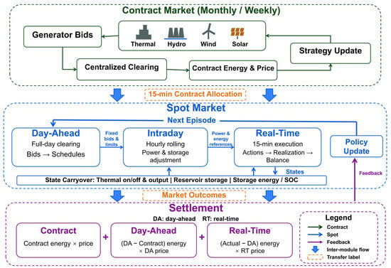
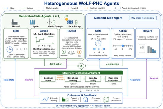
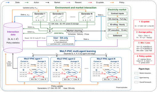
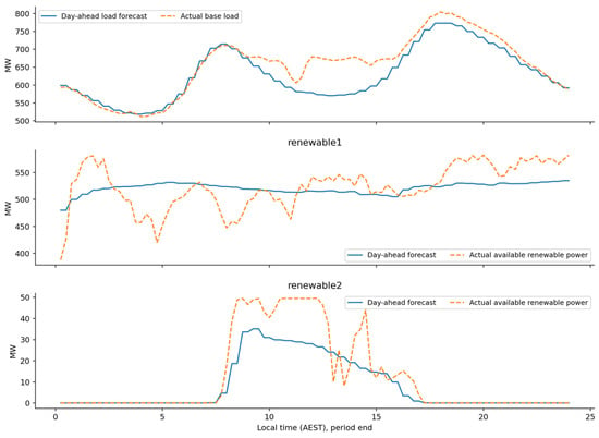
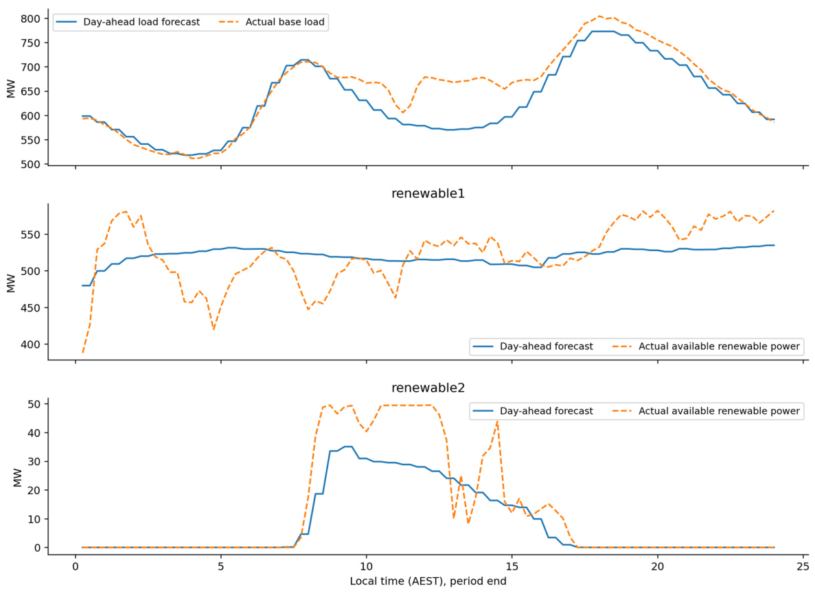
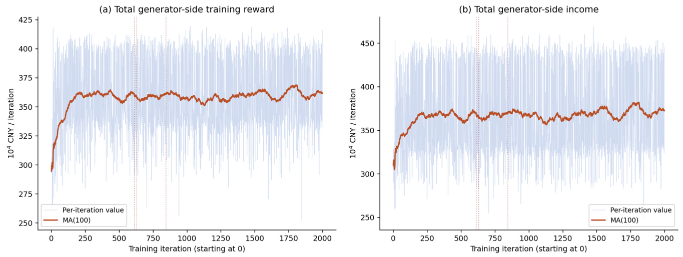
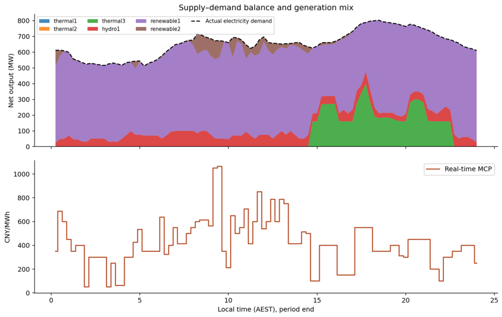
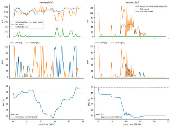
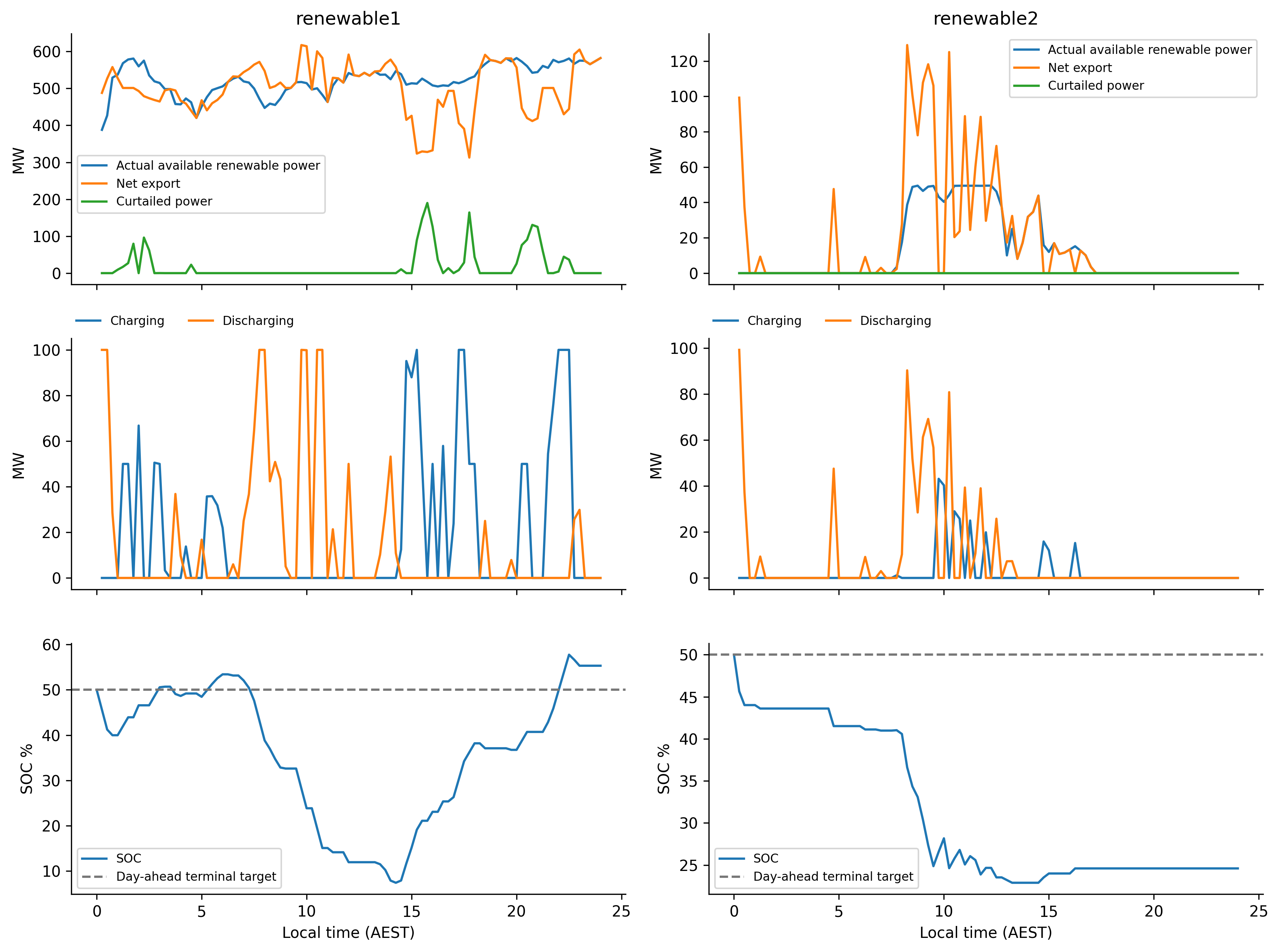
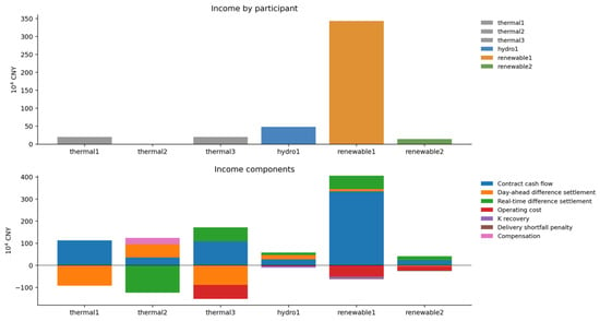
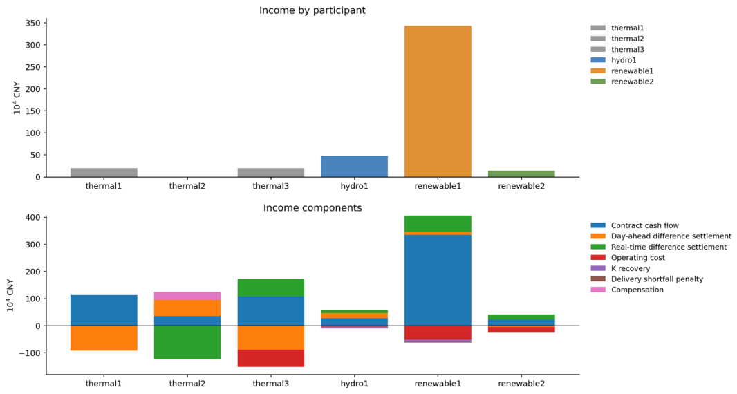
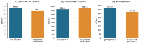
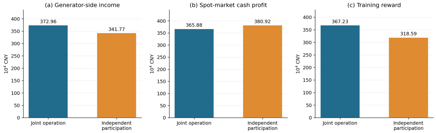
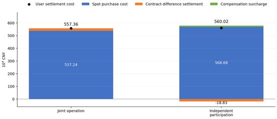
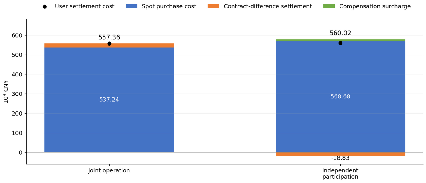
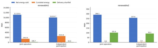
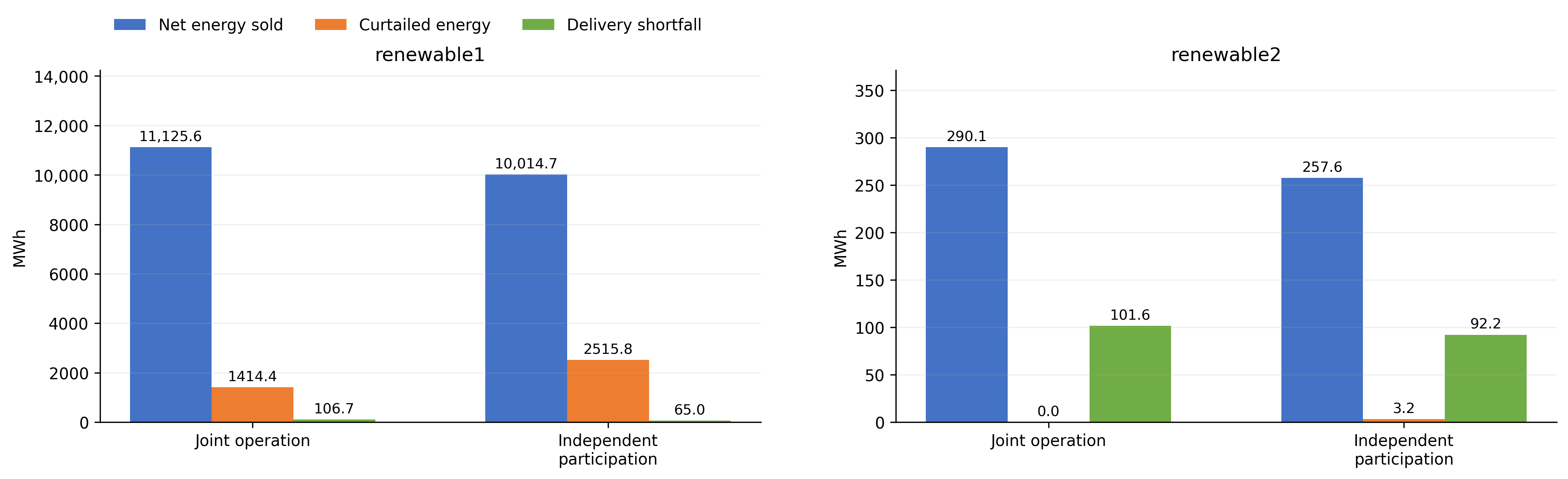
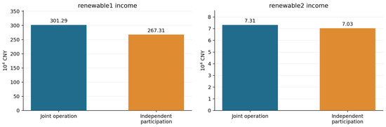
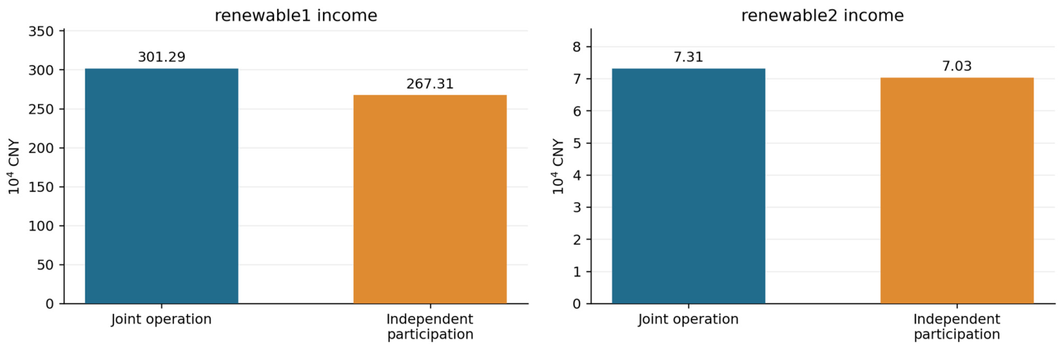
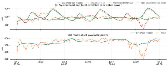
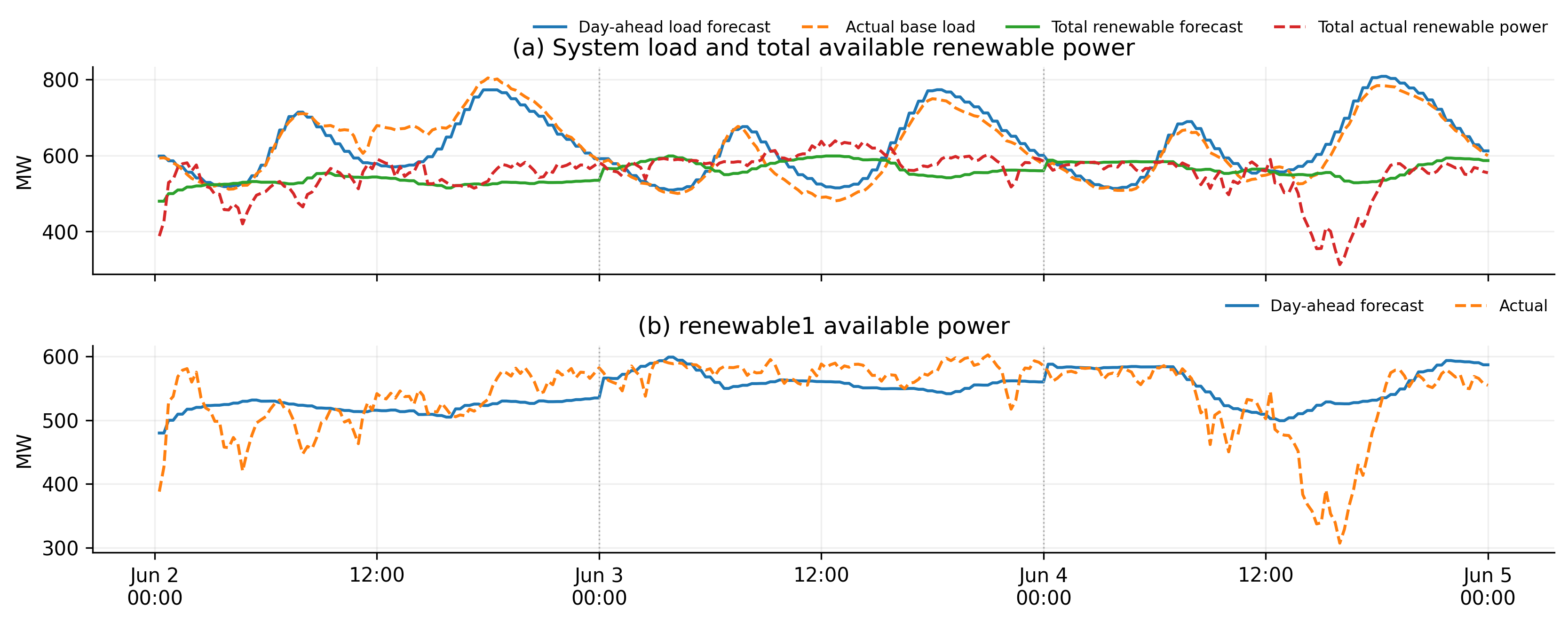
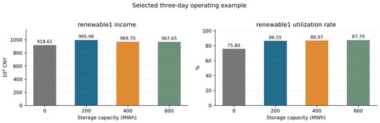
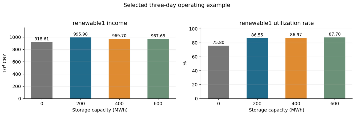
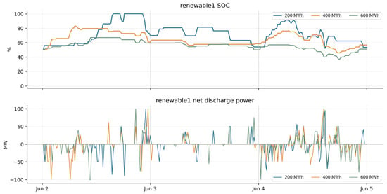
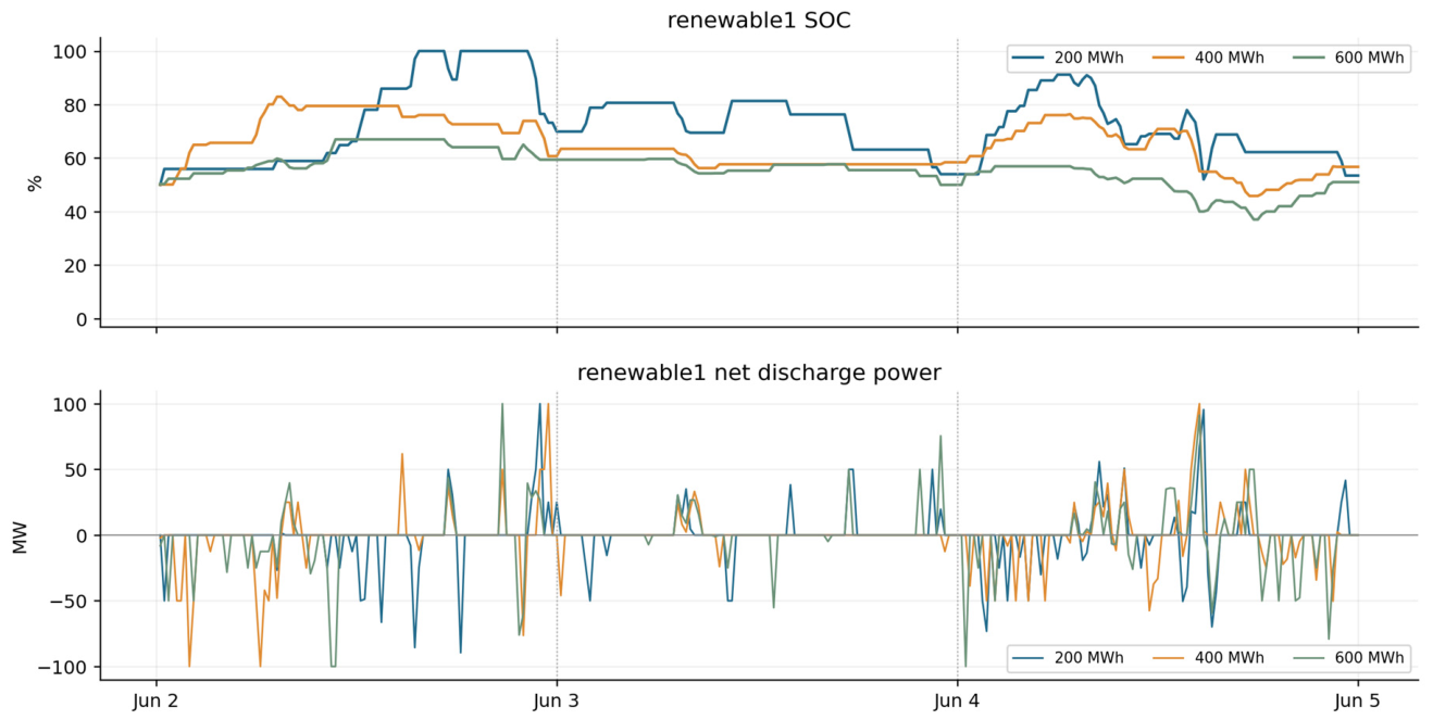

Disclaimer/Publisher’s Note: The statements, opinions and data contained in all publications are solely those of the individual author(s) and contributor(s) and not of MDPI and/or the editor(s). MDPI and/or the editor(s) disclaim responsibility for any injury to people or property resulting from any ideas, methods, instructions or products referred to in the content. |
© 2026 by the authors. Licensee MDPI, Basel, Switzerland. This article is an open access article distributed under the terms and conditions of the Creative Commons Attribution (CC BY) license.