Mass and Aerodynamic Imbalance Estimates of Wind Turbines

Abstract

Due to its effect on the operation time of wind turbines, rotor imbalances of a wind turbine have to be detected early enough. We present a method that determines inhomogeneous mass distributions of the rotor as well as deviations in the pitch angles of the rotor blades from vibrational data only. To this end, a mathematical model connecting the load caused by the imbalances to the resulting vibrations was developed. After discretization, the resulting vibration equation was solved analytically. The inverse problem, i.e., the calculation of the mass and aerodynamic imbalance from vibrational data, was solved by using nonlinear regularization theory. Numerical simulations were performed using artificial vibration data.

1. Introduction

The efficient operation of wind parks calls for a long life time of each wind turbine. As many defects of a turbine can be related to vibrations of the system, the investigation of vibrations caused by rotor imbalances gets more and more attention. The growing size of new wind turbines leads to a more flexible structure and therefore even bigger vibrational amplitudes. Additionally, the operation of large off-shore wind parks requires a careful remote monitoring of imbalances. A well balanced rotor will prevent early fatigue and ensure a safe and economic operation of the wind turbine. Imbalances affect the drive train components as well as the structural health of the turbine [1]. Hence the detection and elimination of imbalances are of vital importance.

There are two main imbalance causes: the so-called mass imbalance arising from inhomogeneous mass distributions caused by, e.g., manufacturing inaccuracies or water inclusions in the blades’ texture, and aerodynamic imbalances, arising, e.g., from errors in the pitch angles or profile changes of the blades. In wind turbines with no Condition Monitoring System (CMS), imbalances are only detected if the vibrations of the turbine are clearly visible, which is only the case if the turbine rotates with a frequency close to the bending eigenfrequency of the turbine, or if there are already damages in the drive train components. If the turbine is equipped with a standard CMS, an increased presence of the rotating frequency and its multiples in the Fourier spectrum can indicate rotor imbalances. In both cases an expert team has to be employed to detect the imbalance location and quantity. In a time consuming process, the team first tries to detect aerodynamic imbalances by using mainly optical methods. If the aerodynamic imbalances have been removed, the remaining vibrations are measured. With a known test mass placed on one blade, a second set of measurements is obtained, and from both measurements together the mass imbalances can be calculated. This process requires not only a lot of time but also expensive manpower. Therefore, it is advantageous to use automatic detection methods. Presently, such methods to detect mass and aerodynamic imbalances by using signal processing methods as well as trend analysis to generate an alarm system require a learning phase performed under faultless condition of the rotor [2]. However, they do not allow to compute the actual value and position of the imbalance. To this aim, vibration measurements with and without test weights as described above are still necessary. To replace this expensive procedure by a new CMS feature is the main goal of the authors work.

First results in that direction were achieved for the observation and reconstruction of mass imbalances only [3]. The mass imbalance reconstruction from noisy vibration measurements was treated as an inverse problem with methods from the regularization theory [4]. To solve an inverse problem, first we have to handle the direct problem of computing the turbine vibrations for a given imbalance. This can be done by using a mathematical model of the turbine that solves the vibration equation with the Finite Element Method (FEM). Although there already exist several models for wind turbines, in [3] we developed a new and comparably simple model for two reasons: Firstly, in order to find a solution for the inverse problem the direct problem has to be solved several times. Thus the computations should be very fast. Secondly, the imbalance identification algorithm should be applicable to a large variety of wind turbine types, which means the model should be adaptable without much effort. In short, in our approach the information from the test run with reference imbalances is replaced by the model information, the additional measurements are superficial due to the mathematical model. However, the model proposed in [3] was restricted to mass imbalances and did not consider aerodynamic imbalances. Moreover, we dealt with a one dimensional model only, i.e., we considered lateral vibrations. Beside axial and torsional vibrations, aerodynamic imbalances also cause vibrations in lateral direction. Thus, neglecting aerodynamic imbalances leads to wrong reconstructions. The resulting error depends on the location of the aerodynamic imbalance and on the rotational frequency, as loads from aerodynamic imbalances depend on the frequency. If the aerodynamic imbalance is located close to the mass imbalance the forces in lateral direction add and we will end up with a reconstructed mass imbalance that is too big. On the other hand, if the aerodynamic imbalance is located opposite to the mass imbalance, we will get a mass imbalance reconstruction that is too small.

In the present paper we consider a model that allows for a reconstruction of both mass imbalances and aerodynamic imbalance caused by deviations in pitch angles at the same time. Since aerodynamic imbalances also cause vibrations in axial directions and torsional vibration around the tower axis, we had to expand our turbine model in these dimensions. To describe the forces and moments from aerodynamic imbalances we have used the blade element momentum (BEM) method. Due to the BEM method, the direct problem of relating the imbalance cause (here the pitch angle deviation and a mass imbalance) to the vibrations of the turbine becomes non-linear. Nevertheless, the regularization techniques for solving the inverse problem also apply to non-linear problems. To ensure a good imbalance reconstruction we observed that the initial value should already be a fairly good guess for the mass imbalance, which we obtained by our old method described above, assuming the absence of aerodynamic imbalances. We reconstructed a good guess for the mass imbalance from the lateral vibrations neglecting the influence from the pitch error. The result is surely not the correct mass imbalance but serves very well as an initial value for the reconstruction of both imbalance causes.

The paper is organized as follows: In Section 2, we will present the system of equations connecting vibrations and imbalances. The mass and stiffness matrices are calculated by a model of the turbine that considers vibration in lateral and axial direction as well as torsional vibrations around the tower axis. The description of forces and moments from mass imbalances is relatively easy, the aerodynamic forces and moments are derived with the BEM method. In Section 3, the vibration equation is solved explicitly, whereas in Section 4, the inverse problem of deriving the imbalances from the vibrations is considered. It results in a nonlinear optimization problem. Section 5 contains examples for the numerical calculation of mass and aerodynamic imbalances from artificial vibration data at the top of the tower.

2. System Equation

Before we can think about reconstructing imbalances from vibration measurements we have to be able to handle the other direction, i.e., for a given imbalance cause we should compute the resulting vibrations of the wind turbine tower. In order to derive appropriate formulas we have to make simplifying assumptions. First we assume that the wind turbine is a flexible shaft (the tower) with an additional mass (the nacelle and the rotor) at the top point, where one part of that mass (the rotor) rotates with a rotational frequency Ω. The movement of such a shaft is described by a Partial Differential Equation (PDE) in time and space. An explicit solution of that equation is seldom possible. Using the Finite Element Method (FEM), the problem can be discretized in space, which results in an Ordinary Differential Equation (ODE) in time. The solution of the ODE is much easier and is a good approximation to the solution of the PDE. The final ODE has the form

$$\begin{array}{c}\hfill \mathbf{M}\ddot{\mathbf{u}}+\mathbf{S}\mathbf{u}=\mathbf{p}\end{array}$$

(1)

where $\mathbf{M}$ denotes the mass or inertia matrix, $\mathbf{S}$ the stiffness matrix, $\mathbf{u}$ the vector of the degrees of freedom and $\mathbf{p}$ the load vector.

For the FEM approach, we divide the tower into elements that are in our case hollow cylinders. We consider movements in lateral or z-direction, in axial or y-direction and torsional movements around the x-axis, see Figure 1 for the coordinate system. There are no movements in x-direction as the tower is supposed to be rigid against shear forces.

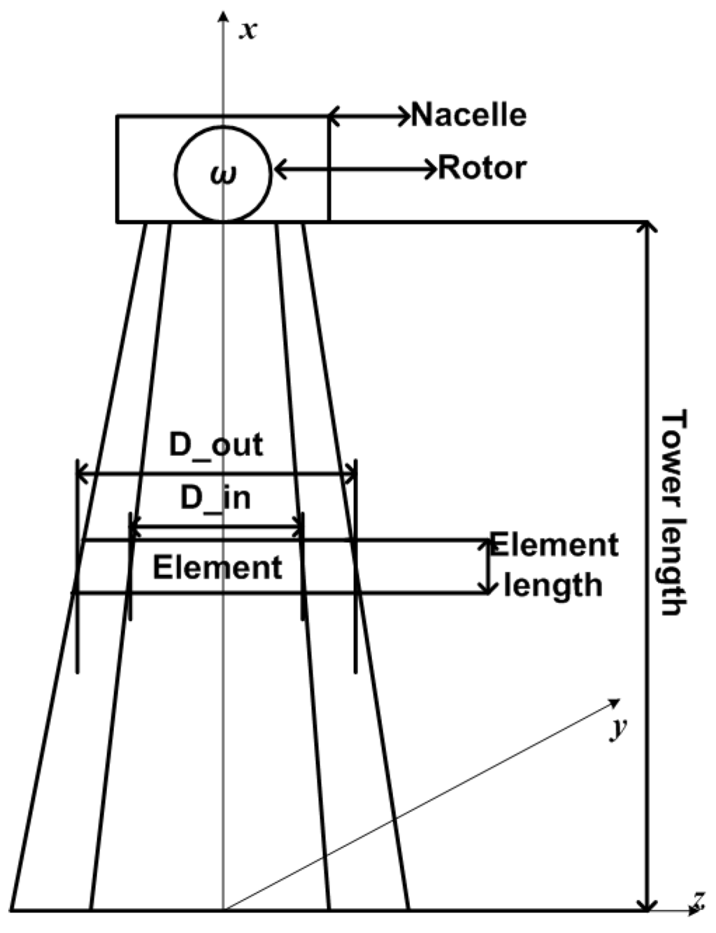
Figure 1. Model of wind turbine.

Figure 1. Model of wind turbine.

2.1. Establishment of the Mass and Stiffness Matrix

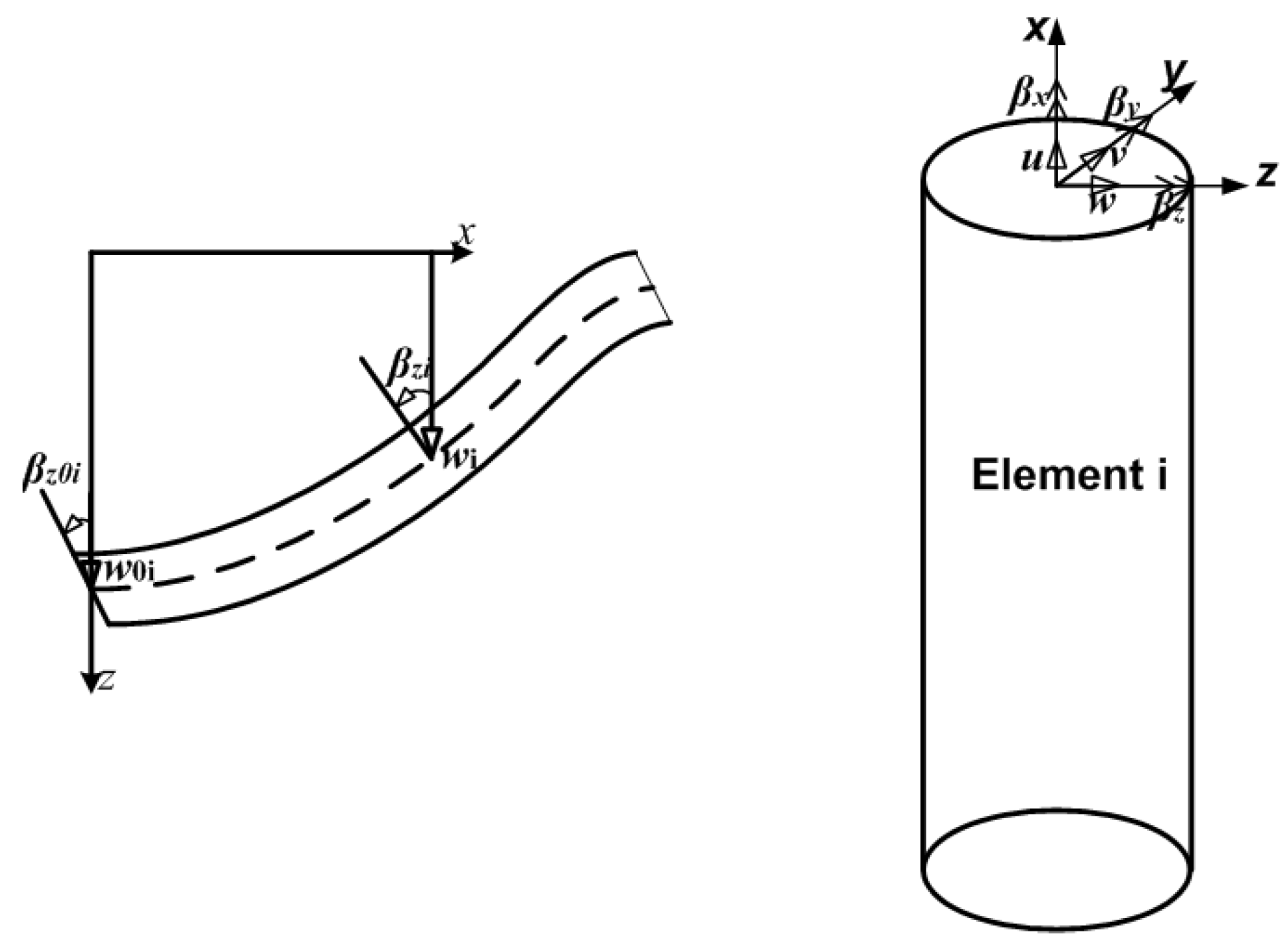
The mass matrix $\mathbf{M}$ and the stiffness matrix $\mathbf{S}$ are derived based on the Ritz method following exactly the way described in [5]. We have divided the tower into N elements with one node at the bottom and one at the top of each element. Each node has five degrees of freedom (DOF),

• $v_i,w_i$ - displacement in y- and z-direction,
• ${\beta }_{xi}$ - cross section rotation (or torsion angle), and
• ${\beta }_{yi},{\beta }_{zi},$ - cross section slope in y- and z-direction,

c.f. Figure 2. We have to take into account the boundary and transition conditions between the elements. The global system displacement vector or vector of DOF is defined by

$$\begin{array}{ccc}\hfill {\mathbf{u}}^T& =& \{v_1,w_1,{\beta }_{x1},{\beta }_{y1},{\beta }_{z1},\cdots ,v_N,w_N,{\beta }_{xN},{\beta }_{yN},{\beta }_{zN}\}\hfill \end{array}$$

where the index number denotes the node number. We assume that the base of the tower does not move. Therefore all DOF of the first node are zero and we have $5N$ entries. The system stiffness matrix and mass matrix are build from the element stiffness and element mass matrices according to the order in the global displacement vector and have the dimension $5N\times 5N$. The mass characteristics from rotor and nacelle have to be added in the mass matrix at the corresponding DOF.

Figure 2. Displacement of a beam.

Figure 2. Displacement of a beam.

2.2. Establishment of the Load Vector

To complete the description of the system Equation (1), it remains to describe the load vector $\mathbf{p}$. Within the scope of this paper, we assume the wind turbine is only affected at the top node of our FE model, and neglect all loads created, e.g., by wind, in other nodes. The forces and moments in the load vector are ordered according to the order of the DOF in the displacement vector $\mathbf{u}$. Hence, the load vector has the form

$$\begin{array}{c}\hfill {\mathbf{p}}^T=(0,\cdots ,0,F_y,F_z,M_x,M_y,M_z)\end{array}$$

(2)

where $F_y$ and $F_z$ denote forces in y- and z-direction, $M_x,M_y$, and $M_z$ are moments of forces or torques w.r.t. the x-, y- and z-axis, respectively. Here $M_y=0$ because we assume mechanical energy related to $M_y$ is transformed into electrical energy.

In the following, we want to consider loads that result from

• inhomogeneous mass distribution of the rotor, and
• aerodynamic forces arising from incorrect pitch angles settings of the rotor blades.

Mass Imbalance

The inhomogeneity of the rotor mass distribution is modeled as point mass m located in the rotor plane at a distance r under an angle ${\theta }_m$ w.r.t. the zero mark at blade A, see Figure 3. The forces caused by this mass are gravity and centrifugal force. With the angular frequency $\omega =2\pi \Omega$, the absolute value for the centrifugal force is given by

$$F_c={\omega }^{2}mr$$

Its projections onto the z- and x-axis are

$$\begin{array}{ccc}\hfill {\left(F_c\right)}_z& =& F_{c}cos(\omega t+\varphi +{\varphi }_m)\hfill \\ \hfill {\left(F_c\right)}_x& =& F_{c}sin(\omega t+\varphi +{\varphi }_m)\hfill \end{array}$$

(3)

Figure 3. Mass imbalance model.

Figure 3. Mass imbalance model.

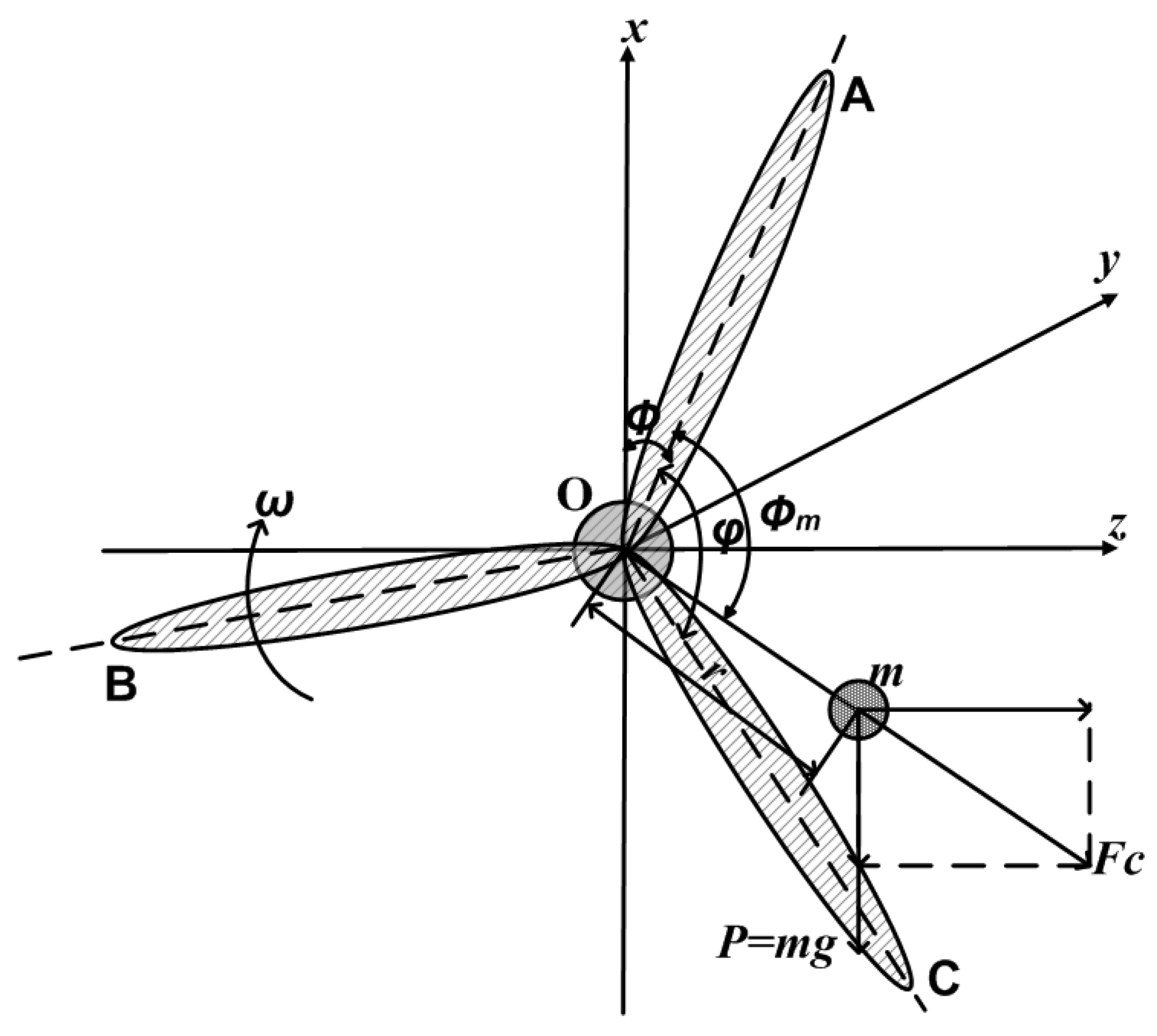
Here, t is time variable, and φ is the angle between blade A and the x-axis. Because the rotational plane has a distance L to the tower, the forces ${\left(F_c\right)}_z$ and ${\left(F_c\right)}_x$ also produce moments around the x- and the z-axes with respect to the tower

$$\begin{array}{ccc}\hfill M_x^1& =& {\left(F_c\right)}_z·L\hfill \\ \hfill M_z^1& =& {\left(F_c\right)}_x·L.\hfill \end{array}$$

(4)

Besides, the gravity force of the point mass also creates a small moment around the z-axis. However, this moment is neglected.

Aerodynamic Imbalance

To describe the aerodynamic loads on a wind turbine, we have employed the well known Blade Element Momentum (BEM) theory, c.f. [7,10]. In the BEM theory, we divide the blades into a finite number of elements which are sections of the blades into annulus segments with the center at the root of the blades. The cross section of each element is called “airfoil”, see Figure 4.

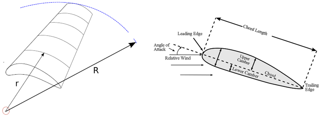
Figure 4. Blade element model with airfoil.

Figure 4. Blade element model with airfoil.

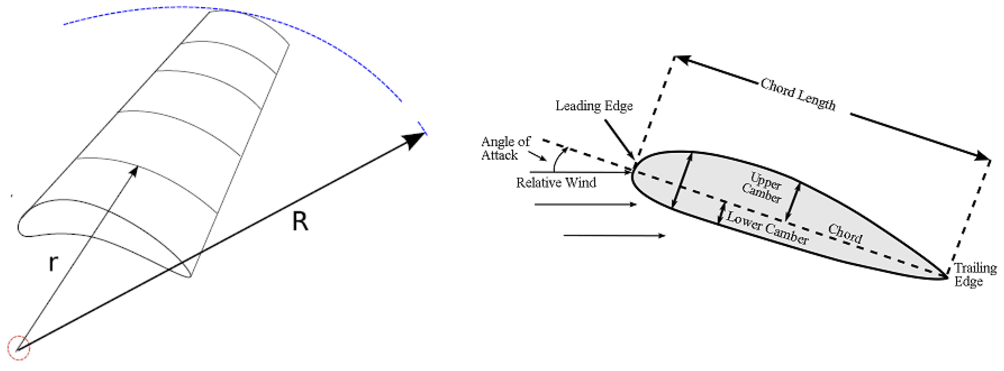
Figure 5. Thrust force on Wind Turbine.

Figure 5. Thrust force on Wind Turbine.

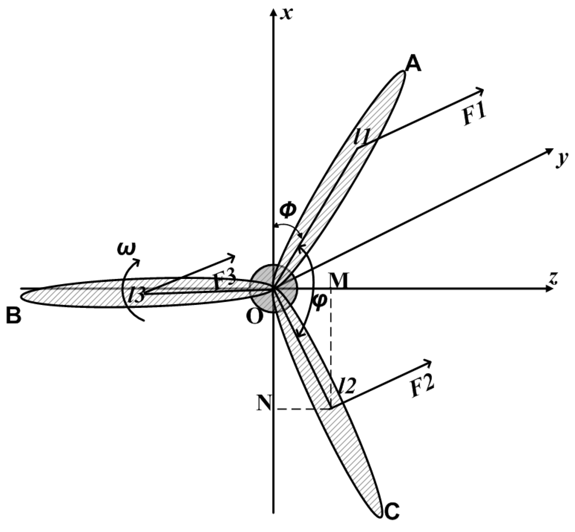
Figure 6. Tangential force on Wind Turbine.

Figure 6. Tangential force on Wind Turbine.

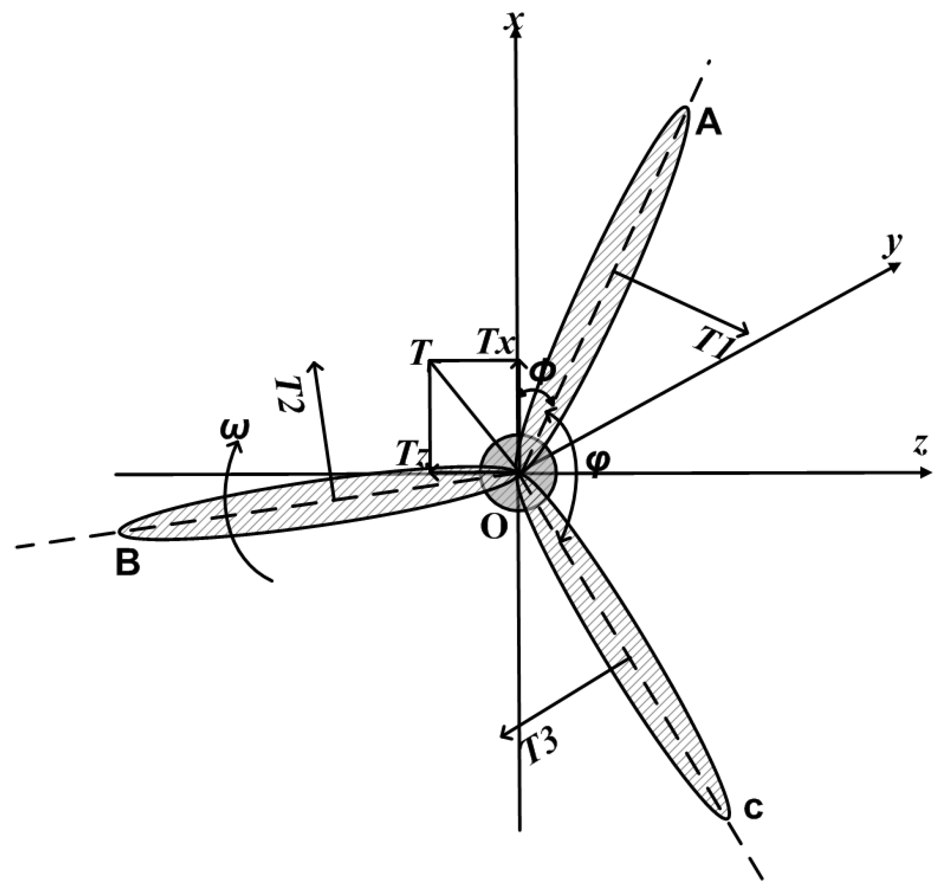
If we are given the airfoil data, the angle of attack of the wind, and the relative wind velocity, as well as a lift and drag coefficient table, we can calculate the normal or thrust forces F and the tangential forces T according to the BEM method, see, e.g., [10], and Figure 5 and Figure 6.

The local pitch angle θ for each blade element, i.e., the angle between chord and the plane of rotation, is the sum of the adjusted pitch angle ${\theta }_p$ at the blades root and the twist of the blade β:

$$\theta ={\theta }_p+\beta .$$

The result of this procedure are forces on each of the blades distributed over all blade elements. However, for manipulation it is more convenient to change the distributed forces on a blade into one equivalent force, see Figure 7.

The distributed forces and the corresponding lengths are calculated by

$$\begin{array}{c}\hfill F={\int }_0^{R}dF=area,l=\frac{{\int }_0^{R}xdF}{F}.\end{array}$$

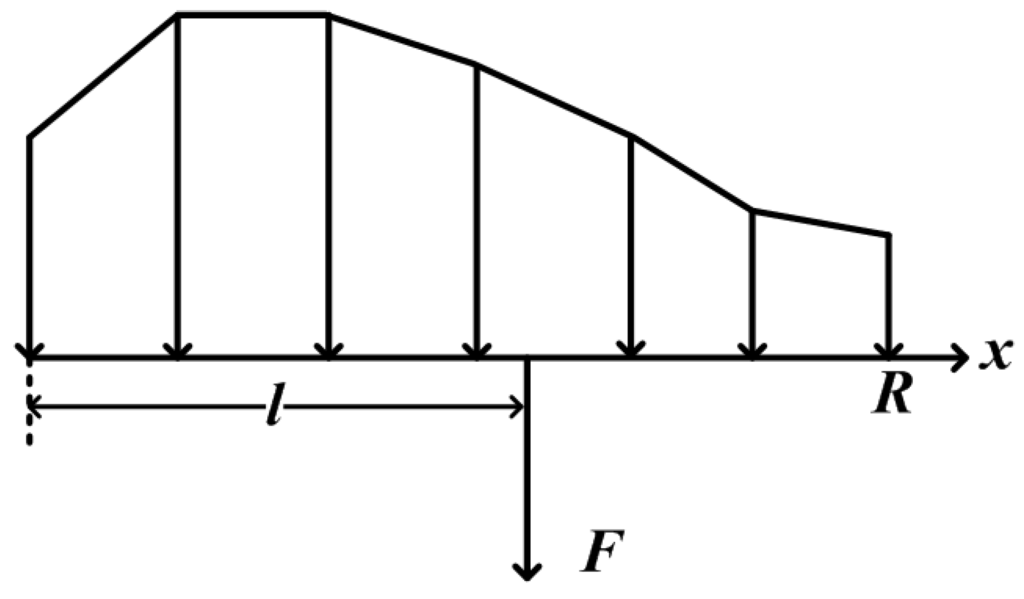
Figure 7. Force equivalent to distributed force.

Figure 7. Force equivalent to distributed force.

Then, the aerodynamic forces can be modeled as three different thrust forces (normal to the rotor plane) and three different tangential forces as shown in Figure 5 and Figure 6. Observing Figure 5 we see that torques caused by $F_1,F_2$ and $F_3$ are given by

$$\begin{array}{ccc}\hfill M_x^2& =& F_1{l}_{1}sin(\omega t+\varphi )+F_2{l}_{2}sin(\omega t+\varphi +\phi )+F_3{l}_{3}sin(\omega t+\varphi +2\phi )\hfill \\ \hfill M_z^2& =& F_1{l}_{1}cos(\omega t+\varphi )+F_2{l}_{2}cos(\omega t+\varphi +\phi )+F_3{l}_{3}cos(\omega t+\varphi +2\phi )\hfill \end{array}$$

(5)

where we denote by $M_x^2$ and $M_z^2$ the torques around the x- and the z-axis on the rotor of the wind turbine and by $\phi =\frac{2\pi }{3}\left({120}^{\circ }\right)$ the angle between the rotor blades. Note that if all blades have the same pitch angle, we have $F_1=F_2=F_3$ and $l_1=l_2=l_3$. This means that the torques $M_x^2$ and $M_z^2$ vanish. In addition, it is easy to see that the sum of $F_1,F_2$ and $F_3$ is the force applying to the rotor in y direction

$$\begin{array}{c}\hfill F_y=F_1+F_2+F_3\end{array}$$

(6)

Observing the Figure 5, we know the total force T is

$$T=T_1+T_2+T_3$$

Projecting T onto z axis and x axis yields

$$\begin{array}{ccc}\hfill T_z& =& T_{1}cos(\omega t+\varphi )+T_{2}cos(\omega t+\varphi +\phi )+T_{3}cos(\omega t+\varphi +2\phi )\hfill \\ \hfill T_x& =& T_{1}sin(\omega t+\varphi )+T_{2}sin(\omega t+\varphi +\phi )+T_{3}sin(\omega t+\varphi +2\phi )\hfill \end{array}$$

(7)

As mentioned before, we have a small distance L between rotor plane and tower, thus $T_z$ and $T_x$ also produces moments around the x- and the z-axes:

$$\begin{array}{c}\hfill M_x^3=T_z·L,M_z^3=T_x·L\end{array}$$

(8)

Load Vector

With the Formulas (3)–(8) the forces and moments from aerodynamic and mass imbalances in (2),

$$\begin{array}{c}\hfill {\mathbf{p}}^T=(0,\cdots ,0,F_y,F_z,M_x,M_y,M_z)\end{array}$$

summarize to:

$$\begin{array}{ccc}\hfill F_y& =& F_1+F_2+F_3\hfill \\ \hfill F_z& =& T_z+{\left(F_c\right)}_z\hfill \\ \hfill M_x& =& M_x^1+M_x^2+M_x^3\hfill \\ \hfill M_z& =& M_z^1+M_z^2+M_z^3\hfill \end{array}$$

(9)

3. Direct Problem

So far we have derived the matrices $\mathbf{M}$, $\mathbf{S}$, and the load vector $\mathbf{p}=\mathbf{p}({\theta }_1,{\theta }_2,{\theta }_3,mr,{\varphi }_m)$. The load $\mathbf{p}$ is a function of the absolute value $mr$ of the mass imbalances, its phase angle ${\varphi }_m$, and the pitch angles ${\theta }_1,{\theta }_2$ and ${\theta }_3$. These five variables determine the forces and moments of forces in (9). The solution of (1) is the sum of the general solution of the homogeneous equation and a particular solution of the inhomogeneous equation with right hand side $\mathbf{p}$. Since $\mathbf{p}$ can be written as a sum of a vector ${\mathbf{p}}_1$ that contains constant entries only, and vectors ${\mathbf{p}}_2$ and ${\mathbf{p}}_3$ that contain the amplitudes of the cos- and sin- terms, respectively, we can solve the inhomogeneous equation analytically. Using standard methods, c.f. [11], we get

$$\begin{array}{cc}\hfill \mathbf{u}\left(t\right)=& (\mathrm{I}-cos({({\mathbf{M}}^{-1}\mathbf{S})}^{1/2}·t)){\mathbf{S}}^{-1}{\mathbf{p}}_1+Re[{(-{\omega }^2\mathbf{M}+\mathbf{S})}^{-1}{\mathbf{p}}_2{e}^{i\omega t}]\\ & +Im[{(-{\omega }^2\mathbf{M}+\mathbf{S})}^{-1}{\mathbf{p}}_3{e}^{i\omega t}]\end{array}$$

(10)

where

$$\begin{array}{ccc}\hfill {\mathbf{p}}_1^T& =& (0,\cdots ,0,F_y,0,0,0,0)\hfill \\ \hfill {\mathbf{p}}_2& =& \left(\begin{array}{c}0\\ \\ 0\\ T_1{e}^{i\varphi }+T_2{e}^{i(\varphi +\phi )}+T_3{e}^{i(\varphi +2\phi )}\\ T_{1}L{e}^{i\varphi }+T_{2}L{e}^{i(\varphi +\phi )}+T_{3}L{e}^{i(\varphi +2\phi )}+{\omega }^{2}mrL{e}^{i(\varphi +{\varphi }_m)}\\ 0\\ F_1{x}_1{e}^{i\varphi }+F_2{x}_2{e}^{i(\varphi +\phi )}+F_3{x}_3{e}^{i(\varphi +2\phi )}\end{array}\right)\hfill \\ \hfill {\mathbf{p}}_3& =& \left(\begin{array}{c}0\\ \\ 0\\ F_1{x}_1{e}^{i\varphi }+F_2{x}_2{e}^{i(\varphi +\phi )}+F_3{x}_3{e}^{i(\varphi +2\phi )}\\ 0\\ T_{1}L{e}^{i\varphi }+T_{2}L{e}^{i(\varphi +\phi )}+T_{3}L{e}^{i(\varphi +2\phi )}+{\omega }^{2}mrL{e}^{i(\varphi +{\varphi }_m)}\end{array}\right)\hfill \end{array}$$

(11)

Therefore, given a mass imbalance $(mr,{\varphi }_m)$ and a set of pitch angles $({\theta }_1,{\theta }_2,{\theta }_3)$ the corresponding vibrations $\mathbf{u}$ are calculated by first determining $\mathbf{p}({\theta }_1,{\theta }_2,{\theta }_3,mr,{\varphi }_m)$, and applying Formulas (10) and (11) afterwards. The forward problem can be solved for every node in our FE-model. However, in view of the inverse problem, where we rely on measured vibration data, we have to consider that vibration sensors are only mounted at a few positions. In practice there will be an acceleration sensor in y-direction, one in z-direction in the middle of the tower top, and, in the best case, one in z-direction at the end of the tower top. From the difference of the last two the torsional movement around the x-axis can be derived. Thus only data for the DOF $(v_N,w_N,{\beta }_{xN})$ will be available. Therefore it is necessary to restrict our solution to these positions or DOF. We denote the restricted vibration by $\mathbf{g}={\mathbf{u}}_{sensor}$. The final forward operator A that relates the imbalances causes to the vibrations is the mapping

$$\begin{array}{c}\hfill \mathbf{g}=A({\theta }_1,{\theta }_2,{\theta }_3,\Delta mr,{\varphi }_m)\end{array}$$

(12)

which performs the calculation of $\mathbf{p}$ summarized in Equation (9), the solution calculation Equation (10) and the restriction step. Unfortunately, this operator is nonlinear due to the BEM method. This property will determine the possible solution methods for the inverse problem of reconstructing $({\theta }_1,{\theta }_2,{\theta }_3,mr,{\varphi }_m)$ from measurements of $\mathbf{g}$.

4. Inverse Problem

4.1. Inverse Problem Description

In recent years the theory of treating (non-)linear ill-posed problems has been well established. For an overview see [4]. For the following, let A be a linear or nonlinear operator between real Hilbert spaces. With given data g, we want to find a solution f of the equation

$$\begin{array}{c}\hfill Af=g\end{array}$$

(13)

The problem is called ill-posed, if the solution f does not depend continuously on the data g. In fact, if we only have noisy data with noise level δ, i.e., $\parallel g^{\delta }-g\parallel \le \delta$, then (provided the inverse $A^{-1}$ exists) $f^{\delta }=A^{-1}{g}^{\delta }$ might be an arbitrarily bad approximation to a solution of (13). To obtain a stable solution, one has to use so called regularization methods. The general idea is to approximate the discontinuous inverse operator by a family of continuous operators $T_{\alpha }$. The regularization parameter α has to be chosen such that ${lim}_{\delta \to 0}\alpha (\delta ,g^{\delta })=0$ holds. For nonlinear operators, equation (13) might have several solutions. Thus we choose the concept of a $\overline{f}$-minimum-norm solution, i.e., we are looking for a solution closest to an a priory given function $\overline{f}$.

A prominent example for a regularization method is Tikhonov regularization. The regularization operator is defined by

$$\begin{array}{c}\hfill T_{\alpha }{g}^{\delta }=f_{\alpha }^{\delta }=arg\underset{f}{min}{J}_{\alpha }\left(f\right)\end{array}$$

(14)

with the Tikhonov functional given by

$$\begin{array}{c}\hfill J_{\alpha }\left(f\right)=\parallel g^{\delta }{-Af\parallel }^2+\alpha {\parallel f-\overline{f}\parallel }^2\end{array}$$

(15)

For the determination of the regularization parameter α, we can use the so called Morozov’s discrepancy principle where α is chosen s.t.

$$\begin{array}{c}\hfill \delta \le \parallel g^{\delta }-A{f}_{\alpha }^{\delta }{\parallel }^2\le c\delta \end{array}$$

(16)

holds [12,13]. For linear operators, the minimizer of the Tikhonov functional can be computed by solving a linear system. In case of a nonlinear operator, optimization methods have to be used additionally to compute a minimizer of (15). A classical approach to minimize the functional $J_{\alpha }\left(f\right)$ is the use of gradient methods. The gradient of the Tikhonov functional is given by

$$\begin{array}{c}\hfill \frac{1}{2}\nabla J_{\alpha }\left(f\right)=A^{\prime }{\left(f\right)}^{*}(Af-g^{\delta })+\alpha (f-\overline{f})\end{array}$$

(17)

where the linear operator $A^{\prime }{\left(f\right)}^{*}$ is the adjoint of the derivative of A at the point f [14]. For other minimization methods we refer to [15,16]. Please note that the above mentioned methods require the derivative of A, which is in our case not available at the moment. Instead we used the Matlab routine, fminsearch. fminsearch uses the simplex search method which is a direct search method. Hence, we can avoid to use numerical of analytic gradients in case that A does not have Frechet derivative. The weak point of this method is the slowness in running time.

5. Computational Results

We have tested the performance of the reconstruction technique for a turbine of the type VESTAS V80-2MW with 100 m tower height and artificial data. We achieved the artificial data by employing the forward operator (12) for a given imbalances situation. The exact vibration data were disturbed by an additive and multiplicative error in order to simulate the noise that arises in measurement. This required the following steps:

• Construction of mass and stiffness matrix using the technical parameters of the V80-2MW (geometry, material properties, first (bending) eigenfrequency 0.255 Hz)
• Setting of a 2 degree pitch angle deviation at the blade C and a mass imbalance of 500 kgm at angle ${\varphi }_m=4\pi /3=4.19$ rad: $[{\theta }_1,{\theta }_2,{\theta }_3,mr,{\varphi }_m]=[0,0,2,500,4.19]$
• Building the load vector $\mathbf{p}$ using formulas (3)–(9) (airfoil code NACA63-421, wind speed 6 m/s, rotational speed 18 rpm, i.e., $\Omega =0.3$ Hz)
• Solving equation (1) using Equation (10)
• Adding $10\%$ noise to the data to simulate the measurements
• Calculate an approximate solution $({\theta }_1^{\prime },{\theta }_2^{\prime },{\theta }_3^{\prime },\Delta m{r}^{\prime },{\varphi }_m^{\prime })$ by minimizing the functional (15) with an appropriate regularization parameter

5.1. Parameter Identification

For our test computations, we set the exact parameters $[{\theta }_1,{\theta }_2,{\theta }_3,\Delta mr,{\varphi }_m]=[0,0,2,500,4.1888]$. We have employed Tikhonov regularization for different kind of data. In a first attempt we used vibration data from all nodes of the model, leading to almost perfect reconstructions. However, in practice only the displacements in y- and z- direction at the top of the tower are available. Reconstructions with these data were done in a second attempt. Those data and their noisy version are presented in Figure 8.

The data was contaminated with $10\%$ noise. Tikhonov regularization with $\alpha ={10}^{-6}$ was used for all reconstructions. The results are displayed in Table 1. The error is split into two parts related to aerodynamical and mass imbalances:

$$\frac{\left|\right|({\theta }_1,{\theta }_2,{\theta }_3)-({\theta }_1^{\prime },{\theta }_2^{\prime },{\theta }_3^{\prime })\left|\right|}{\left|\right|({\theta }_1,{\theta }_2,{\theta }_3)\left|\right|}·100\%,\mathrm{and}\frac{\left|\right|\Delta mr·e^{i{\varphi }_m}-\Delta m{r}^{\prime }·e^{i{\varphi }_m^{\prime }}\left|\right|}{\left|\right|\Delta mr·e^{i{\varphi }_m}\left|\right|}·100\%$$

where $({\theta }_1^{\prime },{\theta }_2^{\prime },{\theta }_3^{\prime },\Delta m{r}^{\prime },{\varphi }_m^{\prime })$ refers to the reconstruction and $({\theta }_1,{\theta }_2,{\theta }_3,\Delta mr,{\varphi }_m)$ is the exact parameter vector.

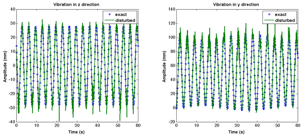
Figure 8. Exact vibration and disturbed vibration in the top of the tower.

Figure 8. Exact vibration and disturbed vibration in the top of the tower.

The results in Table 1 show that the quality of the reconstruction depends on the initial value for the reconstruction. Good initial values, in particular for the mass imbalance, lead to good reconstructions. The main reason for this behavior is the fact that the Tikhonov functional with nonlinear operator might have several, even local minima, where the iteration might get stuck. Therefore, it is crucial to find a good initial value for the minimization routine.

Table 1. Test results with Tikhonov’s regularization algorithm.

Measurements in	Initial value					Noise in %	Result					Aero. Error (%)	Mass. Error (%)
all nodes	0	0	2	500	4	No	0	0	2	500	4.19	0	0
						Yes	0.12	0.05	2.08	500.3	4.19	7.4	0.06
	0	0	0	0	0	No	-6.1	4.57	2.64	307.6	-2.32	382	42
$y,z$ displacement of the top	0	0	0	450	4	No	-0.81	-0.3	1.98	502.9	4.19	43	0.6
						Yes	-0.02	-0.88	1.96	504.9	4.2	44	1.4
	0	0	0	0	0	No	-3.05	-3.05	1.54	83	-2.2	216	84
	0	0	0	420	1.7	Yes	0.37	-0.92	1.75	491.7	4.19	51	1.66

Table 1. Test results with Tikhonov’s regularization algorithm.

Measurements in	Initial value					Noise in %	Result					Aero. Error (%)	Mass. Error (%)
all nodes	0	0	2	500	4	No	0	0	2	500	4.19	0	0
						Yes	0.12	0.05	2.08	500.3	4.19	7.4	0.06
	0	0	0	0	0	No	-6.1	4.57	2.64	307.6	-2.32	382	42
$y,z$ displacement of the top	0	0	0	450	4	No	-0.81	-0.3	1.98	502.9	4.19	43	0.6
						Yes	-0.02	-0.88	1.96	504.9	4.2	44	1.4
	0	0	0	0	0	No	-3.05	-3.05	1.54	83	-2.2	216	84
	0	0	0	420	1.7	Yes	0.37	-0.92	1.75	491.7	4.19	51	1.66

As mentioned in the Introduction, the algorithm proposed in [3], reconstructing mass imbalances only, is inaccurate if we neglect existing aerodynamic imbalances. However, it could provide us with an approximate mass imbalance that serves well as an initial guess for our new algorithm. In Table 1, the last result is calculated by using the initial value from the above mentioned algorithm. The performance of the algorithm was tested on several other examples, see Table 2. In these examples, we have used vibrations of the top of the tower as artificial data. The data were disturbed by 10% noise. Again, the initial values were computed with the algorithm from [3].

Table 2. Test results with Tikhonov’s regularization and fminsearch.

Original Parameters	Initial values	Reconstructed Parameters					Aero. Error (%)	Mass. Error (%)
[0 3 0 350 2.09]	[0 0 0 647 2.09]	-0.25	2.8	0.43	342	2.1	17	2
[2 -2 0 400 1.05]	[0 0 0 798 1.05]	1.99	-0.64	-0.06	402	1.05	48	0.5

Table 2. Test results with Tikhonov’s regularization and fminsearch.

Original Parameters	Initial values	Reconstructed Parameters					Aero. Error (%)	Mass. Error (%)
[0 3 0 350 2.09]	[0 0 0 647 2.09]	-0.25	2.8	0.43	342	2.1	17	2
[2 -2 0 400 1.05]	[0 0 0 798 1.05]	1.99	-0.64	-0.06	402	1.05	48	0.5

5.2. Balancing

For the balancing process, we changed the mass and aerodynamic imbalance in the first example according to the reconstruction (using the last reconstruction in Table 1). Hence, the new pitch angles are given by $[0,0,2]-[0.37,-0.92,1.75]=[-0.37,0.92,0.25]$, and the residual mass imbalance is computed by $500e^{i4\pi /3}+491.7e^{i(4.1929-\pi )}$. Thus, it is $8.5$ kgm located at the phase angle $-2.33$ rad or $226.5^{\circ }$. Note that in practice this is achieved by placing extra weights on the blades. Using these new parameters we have calculated the residual vibration which is plotted in Figure 9.

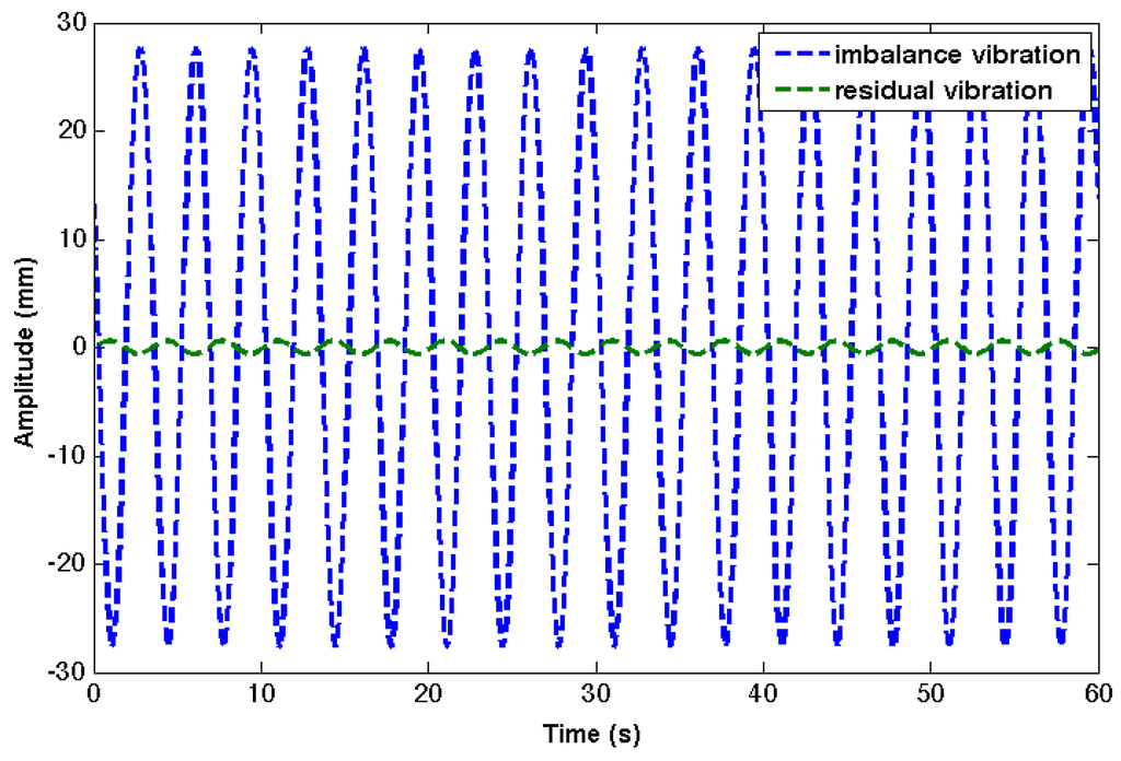
Figure 9. Vibrations in z direction before and after balancing with the computed parameters.

Figure 9. Vibrations in z direction before and after balancing with the computed parameters.

Clearly, the remaining vibrations are much less after balancing.

6. Summary

In this paper we developed an algorithm that can reconstruct both mass imbalances and aerodynamic imbalances arising from pitch angle errors in the rotor of a wind turbine. For the first time it is possible to calculate those values from vibration measurements at the top of the tower only and at the same time. To this end we have developed a turbine model of a Vestas V80-2MW that provides us with the system mass and stiffness matrix. Furthermore, we calculated the load vector that arises in the presence of imbalances using the BEM method. We have solved the vibration equation that connects the vibrations of the system and the load explicitly. This has enabled us to handle the direct problem of computing vibrations in every node of the model for given imbalances, which is necessary to solve the inverse problem by using regularization techniques. With numerical examples we have confirmed that our method works well if the initial guess for the mass imbalance is good enough. This value can be obtained from a previously developed algorithm that works for mass imbalances only. In the future the algorithm has to be tested with data from field measurements. Its successful application will lead to a a new condition monitoring tool that will provide a continuous monitoring of imbalances and a correct distinction between mass and aerodynamic imbalances from pitch angle deviations without using expensive optometrical measurements and vibration measurements with additional test weights.

References

- Ciang, C.C.; Lee, J.; Bang, H. Structural health monitoring for a wind turbine system: A review of damage detection methods. Meas. Sci. Technol. 2008, 19, 122001. [Google Scholar] [CrossRef]
- Caselitz, P.; Giebhardt, J. Rotor condition monitoring for improved operational safety of offshore wind energy converters. ASME J. Solar Energy Eng. 2005, 127, 253–261. [Google Scholar] [CrossRef]
- Ramlau, R.; Niebsch, J. Imbalance estimation without test masses for wind turbines. ASME J. Solar Energy Eng. 2009, 131, 1–7. [Google Scholar] [CrossRef]
- Engl, H.W.; Hanke, M.; Neubauer, A. Regularization of Inverse Problems; Kluwer: Dordrecht, The Netherlands, 1996. [Google Scholar]
- Gasch, R.; Knothe, K. Strukturdynamik 2; Springer: Berlin, Germany, 1989. [Google Scholar]
- Hau, E. Wind Turbines: Fundamentals, Technologies, Application, Economics; Springer: Berlin, Germany, 2006. [Google Scholar]
- Hansen, M. Aerodynamics of Wind Turbines; Earthscan: London, UK, 2008. [Google Scholar]
- Kaltenbacher, B.; Neubauer, A.; Scherzer, O. Iterative Regularization Methods for Nonlinear Ill-Posed Problems; Walter de Gruyter: Berlin, Germany, 2008. [Google Scholar]
- Ahlstroem, A. Aeroelastic Simulation of Wind Turbine Dynamics. PhD Thesis, Royal Institute of Technology, Stockholm, Sweden, 2005. [Google Scholar]
- Ingram, G. Wind turbine blade analysis using the blade element momentum method. In Note on the BEM method; Durham University: Durham, NC, USA, 2005. [Google Scholar]
- Heuser, H.T. Gewöhnliche Differentialgleichungen; B.G. Teubner: Stuttgart, Germany, 1991. [Google Scholar]
- Ramlau, R. Morozov’s discrepancy principle for Tikhonov regularization of nonlinear operators. Numeric. Funct. Anal. Optim. 2002, 23, 147–172. [Google Scholar] [CrossRef]
- Scherzer, O. Morozov’s discrepancy principle for Tikhonov regularization of nonlinear operators. Computing 1993, 51, 45–60. [Google Scholar] [CrossRef]
- Ramlau, R. A steepest descent algorithm for the global minimization of the Tikhonov-functional. Inverse Probl. 2002, 18, 381–405. [Google Scholar] [CrossRef]
- Ramlau, R. On the use of fixed point iterations for the regularization of nonlinear ill-posed problems. J. Inverse Ill-Pos. Probl. 2005, 13, 175–200. [Google Scholar]
- Ramlau, R.; Teschke, G. Tikhonov replacement functionals for iteratively solving nonlinear operator equations. Inverse Probl. 2005, 21, 1571–1592. [Google Scholar] [CrossRef]
© 2010 by the authors; licensee Molecular Diversity Preservation International, Basel, Switzerland. This article is an open-access article distributed under the terms and conditions of the Creative Commons Attribution license (http://creativecommons.org/licenses/by/3.0/).