
A Linearized Large Signal Model of an LCL-Type Resonant Converter


Abstract
: In this work, an LCL-type resonant dc/dc converter with a capacitive output filter is modeled in two stages. In the first high-frequency ac stage, all ac signals are decomposed into two orthogonal vectors in a synchronous rotating d–q frame using multi-frequency modeling. In the dc stage, all dc quantities are represented by their average values with average state-space modeling. A nonlinear two-stage model is then created by means of a non-linear link. By aligning the transformer voltage on the d-axis, the nonlinear link can be eliminated, and the whole converter can be modeled by a single set of linear state-space equations. Furthermore, a feedback control scheme can be formed according to the steady-state solutions. Simulation and experimental results have proven that the resulted model is good for fast simulation and state variable estimation.1. Introduction
Resonant-type dc/dc converters with high-frequency (HF) isolation have been widely used in applications requiring high power density and high efficiency. Until now, many different topologies of resonant tanks have been discussed [1–7], such as the series LC-type, parallel LC-type, series-parallel LCC-type and LCL-type. Two different modulation methods, frequency modulation and phase-shift modulation, are commonly used for the control of resonant dc/dc converters. With the frequency modulation, all switches are working with a fixed duty cycle and a variable switching frequency. A wide spectrum of harmonics naturally results. Meanwhile, a wide range of operating frequencies makes the design of frequency-sensitive components (passive filter, resonant tank, magnetic devices) difficult. The phase-shift modulation is featured with a fixed switching frequency and variable pulse-width. It is easy to implement and free of the main problems of frequency modulation mentioned before. Modeling a converter can reveal the interrelation among each parameter and give insight into the operation in the steady state and the dynamics. However, modeling of HF-isolated resonant-type dc/dc converters is difficult, because of a high number of reactive components and the non-linear switching behavior [8,9]. Small signal modeling is used to design a closed-loop controller for stable operation by investigating the system response to the small perturbation near a steady-state working point [10–13]. It can be based on the discrete time domain or the multiple frequency technique. Normally, discrete-time domain-based modeling is limited to a low order system. The multiple frequency method converts ac signals to dc signals at different frequencies and could generate a theoretically accurate model [14]. Although a small signal model is good for closed-loop design, it cannot provide a quick estimation of the converter state variables with large variation, especially when the converter has a larger operation range. By using the describing function, a nonlinear large signal model was proposed in [15], which resulted in non-linear controllers [16]. While nonlinear control is robust and accurate, it is complex and hard for practical implementation. In [17,18], a series-parallel LCC resonant converter with an inductive output filter is modeled with multiple frequency modeling and averaged state-space techniques. The obtained linearized large signal model can be linearized and results in a natural closed-loop control.
In this paper, an LCL resonant dc/dc converter with a capacitive output filter is selected to be modeled in this paper. The reason is that the LCL-type resonant tank is proven to be helpful for maintaining zero-voltage switching and high efficiency for a wide load range [19–24]. With a capacitive output filter, the voltage ringing on the diode rectifier due to an inductive output filter could be eliminated. To the best knowledge of the author, there is a lack in the literature of dedicated work for modeling the phase-shifted LCL resonant converter. The main features can be concluded as an aggregated linearized model for the phase-shift LCL resonant converter with a capacitive output filter constructed using fundamental harmonics approximation. Compared with previous works using the linear or nonlinear model, the obtained model could be used for fast estimation of the converter operation states without many complicated calculations involved. The obtained natural feedback control scheme is simple and straightforward and can be utilized for accurate closed-loop control if an additional simple controller (like a proportional-integral or proportional-integral-differential controller) is used.
The paper is organized as follows. In Section 2, The HF-isolated LCL resonant dc/dc converter is modeled in two stages according to different operating frequencies. A unified state-space model with a non-linear inner link is then created by combining two sub-models together. A natural linear feedback control is then obtained by aligning the transformer voltage with an axis in a synchronous rotating frame. Verification of the universal model and the feedback control is performed by MATLAB simulation and experimental testing on a laboratory converter prototype.
2. The LCL-Type Resonant dc/dc Converter with a Capacitive Output Filter
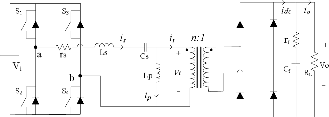
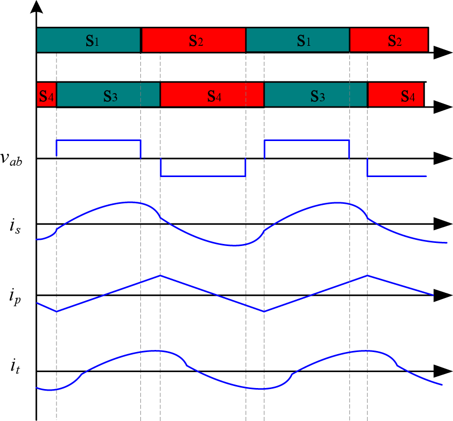
In Figure 1, the circuit diagram of an HF-isolated LCL-type resonant dc/dc converter is presented. Figure 2 illustrates its steady-state operation waveforms. The input dc voltage Vi is converted into an HF ac voltage vab by means of an HF full-bridge inverter. All switches are working with a fixed frequency. The two switches in each inverter leg are operated alternatively with a duty cycle slightly lower than 50%. There is a phase-shift between the two inverter legs, which is modulated to regulate the output voltage at different load level. Thus, the HF bridge inverter output voltage vab is a quasi-square wave. The series resonant frequency defined by the LCL tank is normally designed to be quite close to the switching frequency ωs. Therefore, the induced tank current is is nearly sinusoidal. The HF transformer voltage vt is a square wave due to the assumption of a large capacitive output filter. The parallel inductor current ip is a triangular waveform, which is helpful to extend the ZVS (zero-voltage switching) operation range as the load varies. The resulted transformer current it is rectified to a pulsing dc output current idc through the HF diode rectifier. The HF ac harmonics inside idc are then filtered out by the capacitive filter Cf. The leakage inductance of the transformer is included in the series resonant inductance Ls. The magnetic inductance of the transformer can be integrated with the parallel inductance Lp by proper magnetic design. The equivalent resistance rs combines the winding resistance of the series inductor and the HF transformer, the on-state resistance of switches and diodes. rf is the equivalent series resistance (ESR) of the filter capacitor.
3. A Nonlinear Model Based on a Two-Stage Equivalent Circuit
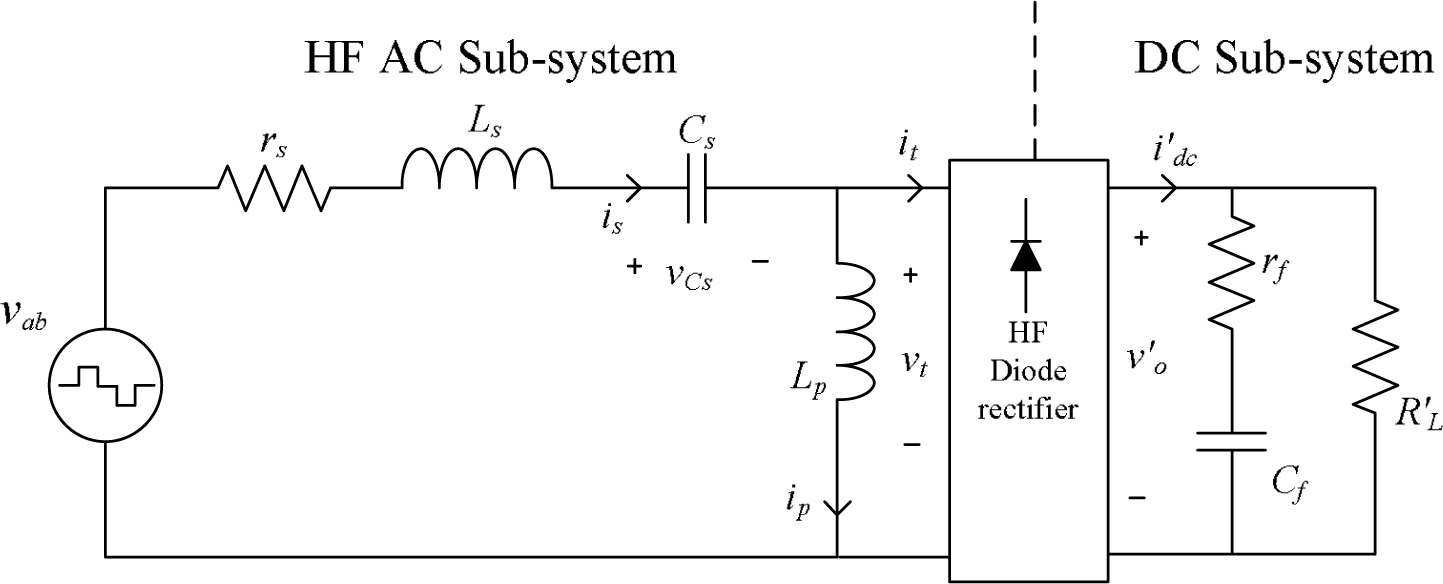
To perform the modeling of the LCL-type resonant converter, a simplified equivalent circuit of the LCL-type converter with the active switch network and the HF transformer removed is illustrated in Figure 3. All quantities have been reflected on the primary side, and the reflected secondary parameters are marked with a superscript “″”. The snubber effect and switching transients are neglected.
As a multi-stage conversion system, this converter can be divided into two sub-systems with the HF diode bridge as the boundary: the HF ac sub-system and the dc sub-system. In the following analysis, mathematical models will be constructed for each sub-system and then linked together according to the nature of the diode rectifier.
3.1. Modeling of the HF AC Sub-System Using Phasor Transformation
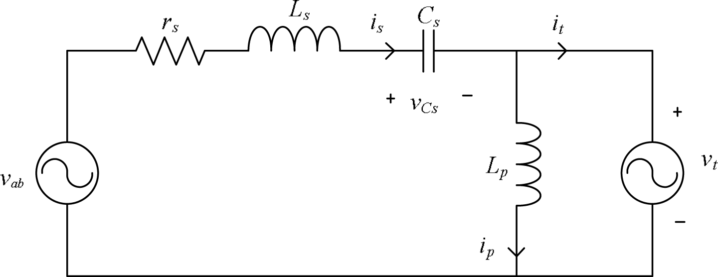
As seen from Figure 4, the HF ac sub-system consists of two voltage sources and an impedance network. The right-side voltage source vt is the primary-side voltage of the HF transformer (also the voltage across the parallel inductor Lp), which stems from the ripple-free output voltage via the operation of the HF diode bridge. The set of differential equations describing the dynamics of the three reactive components can be written as:
The transformer current is obtained as:
As mentioned before, the inductor current is and capacitor voltage vCs are nearly sinusoidal due to the close-to-resonance operation. Additionally, the HF inverter output voltage vab, the transformer voltage vt, the parallel inductor current ip and the transformer current it are all ac-dominant signals. Therefore, it is reasonable to use only the fundamental components to approximate each ac voltage and current in this converter. To explore the dynamics of the HF sub-system, the set of state equations are converted into the phasor domain firstly:
For each sinusoidal voltage or current, its corresponding phasor can be expressed in a d–q coordination system rotating with an angular speed ωs. For example:
The d-axis and q-axis values are orthogonal functions of the time t and would be constants in the steady state. The components along the d-axis and q-axis can be evaluated as:
By using such a phasor transformation, all ac signals in Equations (5)–(8) can be written as phasors in the d–q rotating frame:
Thus, Equations (5)–(8) can be decoupled along the d-axis and q-axis, respectively, by using Equations (12)–(17).
Equations (18)–(25) can be reorganized into the standard form of the state-space equations:
3.2. Modeling of the DCSub-System
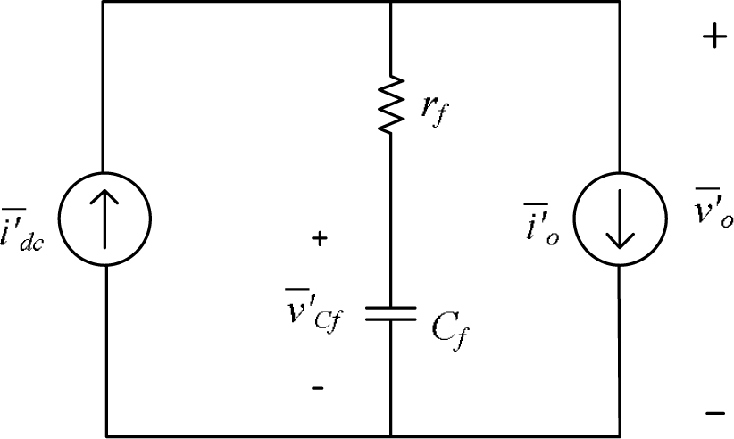
The equivalent circuit of the dc sub-system is presented in Figure 5. All voltages and currents in this subsystem are dc dominant and are represented by their average values only. The left current source is the average output current of the diode rectifier, and the right one is the average load current is the average output voltage. is the average filter capacitor voltage. The differential equations describing the dc sub-system are concluded as:
Following a similar principle as in the last section, the state variable vector , the input vector and the output vector for the dc sub-system can be defined as:
Thus, the standard state-space model of the dc sub-system looks like:
3.3. Modeling of the Diode Bridge Rectifier
According to the waveforms in Figure 2, the function of the diode rectifier is to convert the sinusoidal it into a pulsing dc current and to convert the square-wave vt into a nearly ripple-free . If only average values of the dc-dominant signals are considered in the dc sub-system, the relationship across the diode bridge can be concluded as follows: the current source (one of the inputs of the dc sub-system) is the average of the rectified current it (the output of the ac sub-system), and the output voltage is the average of the rectified fundamental transformer voltage vt:
With the assumption of a lossless power transfer, the power on both sides of the diode bridge should be balanced as:
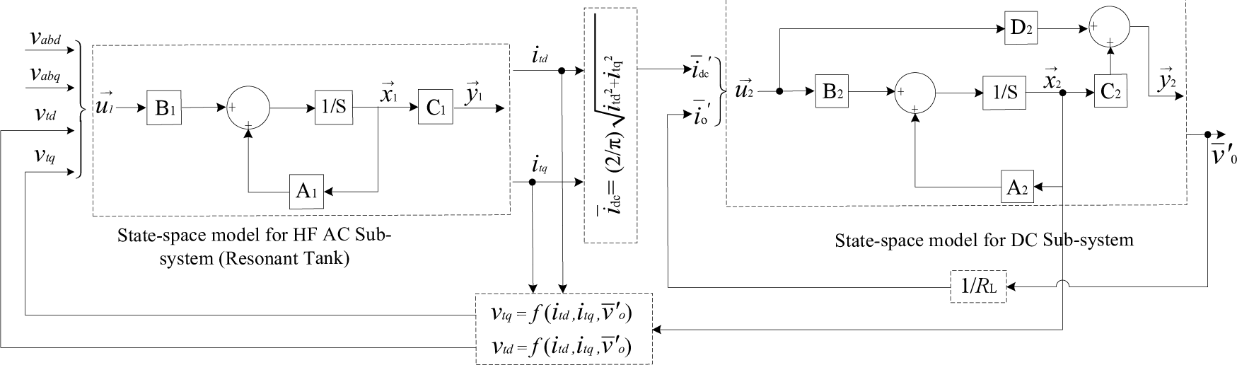
By means of Equations (43)–(45), the two models in each stage can be linked together now as shown in Figure 6. Due to the existence of the square root operation in Equation (43), the combined model of the LCL-type resonant converter is nonlinear.
3.4. Steady-State Solutions of the Nonlinear Model
The steady-state solutions of all state variables could be found by simply setting the derivative vectors of state variables in Equations (26), (27), (40) and (41) to be zero.
The steady-state solutions of the HF ac sub-system are given as:
Based on Equation (46), the input voltage Vab should satisfy the following conditions to get the particular It and Vt in the steady state:
The steady-state solutions of the dc sub-system are given as:
The relationship described in Equations (43)–(45) is still valid for those steady-state values and can be combined with Equations (49)–(51) to find any particular parameter.
4. A Linearized Model of the LCL-Type Resonant Converter
Equations (49) and (50) reveal that the required components of Vab along the d-axis or q-axis are decided by both the d-axis component and q-axis component of Vt and It. In order to decouple the d–q interconnection, vt is assumed to be on the d-axis, i.e., vt = vtd, vtq = 0. With this assumption, the following results can be gotten from Equations (43)–(45):
It can be seen that in the steady state, the d–q components of Vab are decided by Itd and Vtd only, which, in turn, are proportional to the load current and the load voltage, respectively. If the equivalent parasitic resistance rs is neglected, Equations (56)–(57) can be reduced further into:
It is seen that the control of the output voltage and the output current are decoupled, and they are decided by Vabq and Vabq, respectively.
Equations (53) and (54) are also actually the necessary conditions to meet the requirement for linearization of the relationship between two sub-systems, i.e., only such an input voltage Vab can result in It = Itd; Vt = Vtd. Therefore, a natural feedback scheme can be formed in the dynamics. The actual controllable input voltage vab could be decided by:
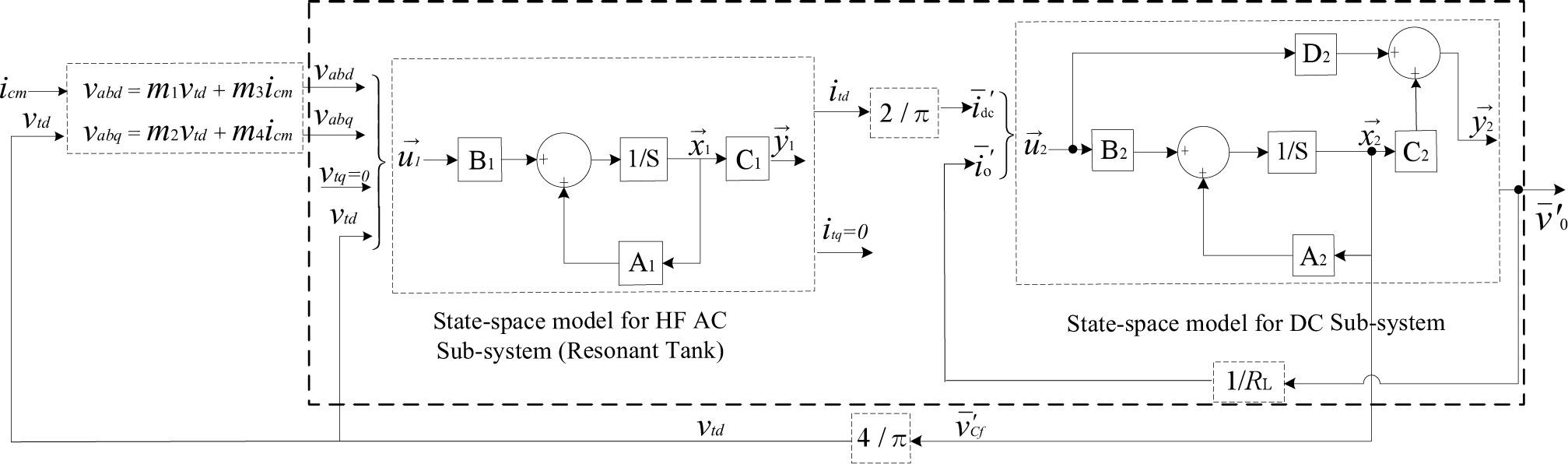
The term including vtd in each equation is the weighted state feedback for linearization. The obtained linearized model of the LCL-type resonant converter is given in Figure 7. In this feedback control scheme, the only parameter needed to be sampled is the output voltage.
Additionally, the two sub-systems can be described using only one set of state-space equations.
The new state variables vector x(t), input vector u(t) and output vector y(t) are defined as:
5. Validation through Simulation and Experimental Results
In order to evaluate the accuracy of the developed model, the simulation and experimental results are presented in this section. In Table 1, the specifications of the converter to be investigated are presented. The design of the converter is based on the steady-state analysis using the Fourier series approach presented in [19]. For the selection of the design parameters and design procedures, the reader can refer to [19], too.
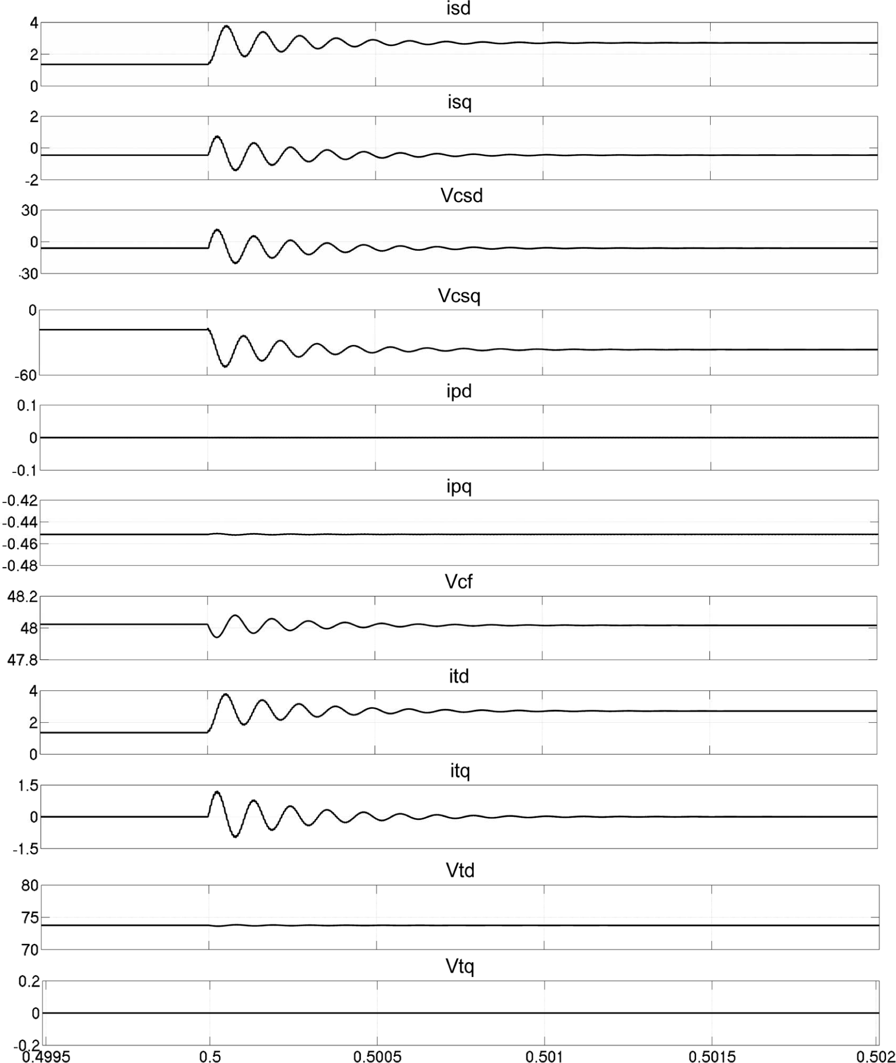
At first, simulation on the combined model in Equation (58) is performed in MATLAB/Simulink. The converter starts with the half load (the control input icm = 1.357 A and load resistance RL = 46.08 Ω at t = 0 s). The transient response is then investigated by changing the load level from half load to full load (ict = 2.713 A, RL = 23.04 Ω) at t = 0.5 s. The resulting plots are presented Figure 8. It is observed that itd and isd are exactly the same, and they follow the change of the current command icm. In the steady state, vCsq, vCsd are proportional to isd, isq, respectively. As predicted, itq and ipd are nearly zero, except for the transient of load-changing. isq is equal to ipq in the steady state when the itq settles down to zero. The transformer voltage vtd and output voltage remain almost unchanged during the transient of load-changing.
A lab prototype of the LCL converter with the same specifications was built and tested, too. One pair of ETD39 cores (material N97, EPCOS AG, Munich, Germany) is used as the core of the HF transformer. The windings are made of multi-thread litz wire with a turn ratio of 12:11. Both the series inductor and the parallel inductor are built with a toroidal core (material Ni–Fe permalloy). The main switches used in the full bridge are HEXFET® power MOSFET IRFR4620 (International Rectifier, El Segundo, CA, USA). Additionally, the power diodes used in the HF rectifier are MUR1560 with ultrafast recovery time. To take the leakage and magnetic inductance of the HF transformer, the parallel inductor Lp is put on the secondary side of the HF transformer. The calculation of the feedback control and the generation of gating signals are implemented in an Altera Cyclone II FPGA development board. As the main switch has a low switching delay, the deadband of gating signals is selected at 150 ns.
It should be noted that the control scheme is not a proper closed-loop control, even though a natural feedback control exists. Normally, most of the load is the constant-voltage type, so that it is the converter output voltage rather than the output current that should be kept constant when the load resistance changes. However, the control input in this feedback control scheme is the output current, which means that in order to keep output voltage constant, the current command should be adjusted instantly whenever a change of load resistance happens. Thus, in practical applications, the current command should be determined by means of an extra feedback output voltage or current controller, whose design deserves more work in the future. For the actual test reported in this paper, a constant voltage-type load is used instead of a resistive load to evaluate the accuracy of the natural feedback control scheme only.
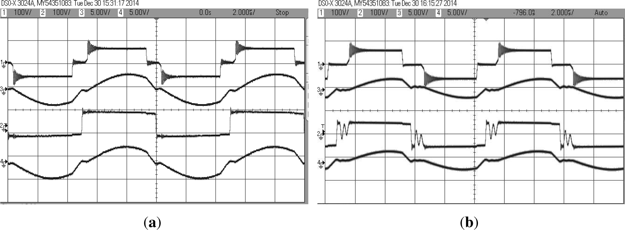
The steady-state experimental waveforms with open-loop control are presented in Figure 9 for full load and half load operation. vAB is a quasi-square wave voltage with a different pulse width when the load level varies. vt is a full square-wave voltage at full load. However, it has a ringing part at partial load, in which the secondary current is almost zero, and there is a resonance between the three resonant tank components. In spite of this irregularity, it can be seen that vt and it are still in phase, which indicates the correctness of the previous assumption made in Section 4.
In Table 2, a comparison is also made for RMS (root-mean-square) values of important state variables in the steady state between the simulation results and experimental test. A certain degree of match for most of parameters can be found from Table 2. The difference originates from two parts: the non-ideal components in the experiment and the approximation analysis approach using fundamental sinusoidal signals only. Generally, the deviations in partial load are higher than those in the full load condition. The reason is that there are more high-order harmonics in each quantity under the partial load condition. Furthermore, the deviation of vt is much higher than the others, because vt is a square-wave signal, while the others assemble sinusoidal signals.
Then, the closed-loop control with the natural feedback scheme is tested by a similar transient test as in the simulation. The four curves shown in Figure 10 are the series resonant current is, the resonant capacitor voltage vCs, the transformer voltage vt and current it measured from the secondary side. With the change of current command, the indicators of the load level (it) and resonant tank parameters (is, vCs) rose from half load operation to full load operation. The settling time is approximately 1.5 ms, which is longer than the simulation results. The power level control is not accurate, with 7% and 11% at full load and half load conditions, respectively. The reason can be be attributed to: (1) the approximation used in the modeling procedure; (2) the error in measurement and estimation of the parameters used in the calculation (like Ls, Cs, rf, rs); (3) other non-ideal conditions in the real test (like the effect of the deadband of gating signals, etc.). To eliminate the apparent steady-state error, an extra compensation controller is needed to generate accurate gating signals. Since the natural feedback scheme itself is linear, a low-order PI or PID controller might be sufficient for better performance.
6. Conclusions
In this paper, the proposed work addressed the modeling of an HF-isolated LLC resonant converter with a capacitive output filter. The modeling technique combines the simple sinusoidal approximation in a synchronous rotating frame with the conventional dc state-space averaging approach. Based on the main operating frequency in two different conversion stages in the converter, two state-space models for high-frequency ac and dc are derived and linked with a non-linear relationship. Then, by aligning the synchronous rotating reference frame for the HF ac stage with one component of the transformer voltage, the inter-stage link is linearized, so that both HF ac and dc variables can be combined together to generate a unified state-space model. A weighted state feedback scheme is naturally obtained according to the steady-state solutions. Both simulation plots and experimental results show that the developed linear aggregated model can be used to estimate the operation condition of the converter with easy calculation and an acceptable accuracy level. Although the natural state feedback control is not quite accurate for power regulation due to the approximation in the analysis, it lays a good base for further precise closed-loop control, since no additional compensation controllers are used now. In future work, further efforts are needed to design extra voltage/current controllers to compensate for the errors introduced in the theoretical calculation and to improve the stability.
Acknowledgments
The authors would like to thank the financial support from the Science and Technology Development Fund of Macau (FDCT) under Grant Agreement No. 067/2011/A.
Author Contributions
Mr. Hong-Yu Li was responsible for the theoretical derivation and proving and for paper writing. The main contribution of Xiaodong Li was the planing, coordination and consultation of the whole project. Mr. Ming Lu made a contribution to the circuit implementation and microcontroller programming. Mr. Song Hu made a contribution to the data processing, LaTeX editing and proof reading.
Conflicts of Interest
The authors declare no conflict of interest.
References
- Steigerwald, R.L. A comparison of half-bridge resonant converter topologies. IEEE Trans. Power Electron. 1988, PE-3, 174–182. [Google Scholar]
- Batarseh, I. Resonant converter topologies with three and four energy storage elements. IEEE Trans. Power Electron. 1994, 9, 64–73. [Google Scholar]
- Bhat, A.K.S.; Dewan, S.B. A generalized approach for the steady state analysis of resonant inverters. IEEE Trans. Ind. Appl. 1989, 25, 326–338. [Google Scholar]
- Li, X.D.; Bhat, A.K.S. Analysis and design of high-frequency isolated dual-bridge series resonant dc/dc converter. IEEE Trans. Power Electron. 2010, 21, 850–862. [Google Scholar]
- Li, X.D.; Li, H.-Y.; Hu, G.-Y.; Xue, Y. A bidirectional dual-bridge high-frequency isolated resonant DC/DC converter, Proceedings of the 8th IEEE Conference on Industrial Electronics and Applications (ICIEA), Melbourne, Australia, 19–21 June 2013; pp. 49–54.
- Li, X.D.; Li, H.-Y.; Hu, G.-Y. Modeling of the fixed-frequency resonant LLC DC/DC converter with capacitive output filter, Proceedings of the 5th IEEE Energy Conversion Congress and Exposition (ECCE), Denver, CO, USA, 15–19 September 2013.
- Hu, G.-Y.; Li, X.D.; Luan, B.-Y. A generalized approach for the steady-state analysis of dual-bridge resonant converters. Energies 2014, 7, 7915–7935. [Google Scholar]
- Ye, Z.; Jain, P.K.; Sen, P.C. Phasor-domain modeling of resonant inverters for high-frequency AC power distribution systems. IEEE Trans. Power Electron. 2009, 24, 911–923. [Google Scholar]
- Rim, C.T. Unified general phasor transformation for AC converters. IEEE Trans. Power Electron. 2011, 26, 2465–2475. [Google Scholar]
- Batarseh, I.; Siri, K. Generalized approach to the small signal modelling of DC-to-DC resonant converters. IEEE Trans. Aerosp. Electron. Syst. 1993, 29, 894–909. [Google Scholar]
- Agarwal, V.; Bhat, A.K.S. Small signal analysis of the LCC-type parallel resonant converter using discrete time domain modeling. IEEE Trans. Ind. Electron. 1995, 42, 604–614. [Google Scholar]
- Ye, Z.; Jain, P.K.; Sen, P.C. Modeling of high frequency resonant inverter system in phasor domain for fast simulation and control design, Proceedings of the 39th Annual IEEE Power Elctronics Specialists Conference, Rhodes Island, Greece, 15–19 June 2008; pp. 2090–2096.
- Sanders, S.R.; Noworolski, J.M; Liu, X.Z.; Verghese, G.C. Generalized averaging method for power conversion circuits. IEEE Trans. Power Electron. 1991, 6, 251–259. [Google Scholar]
- Ye, Z.; Jain, P.K.; Sen, P.C. Multiple frequency modeling of high frequency resonant inverter system, Proceedings of the 35th Annual IEEE Power Elctronics Specialists Conference, Aache, Germany, 20–25 June 2004; pp. 4107–4113.
- Agarwal, V.; Bhat, A.K.S. Large signal analysis of the LCC-type parallel resonant converter using discrete time domain modeling. IEEE Trans. Power Electron. 1995, 10, 222–238. [Google Scholar]
- Sosa, J.; Castilla, M.; Miret, J.; de Vicuña, G.L.; Matas, J. Modeling and performance analysis of the dc/dc series-parallel resonant converter operating with discrete self-sustained phase-shift modulation techniques. IEEE Trans. Ind. Electron. 2009, 56, 697–705. [Google Scholar]
- Aboushady, A.A.; Ahmed, K.H.; Finney, S.J.; Williams, B.W. State feedback linearized model for phase-controlled series-parallel resonant converters, Proceedings of the 37th Annual Conference on IEEE Industrial Electronics Society, Melbourne, Australia, 7–10 November 2011; pp. 1590–1595.
- Aboushady, A.A.; Ahmed, K.H.; Finney, S.J.; Williams, B.W. Linearized large signal modeling, analysis, and control design of phase-controlled series-parallel resonant converters using state feedback. IEEE Trans. Power Electron. 2013, 28, 3896–3911. [Google Scholar]
- Bhat, A.K.S. Analysis and design of a fixed-frequency LCL-type series-resonant converter with capacitive output filter. IEE Proc. Circuits Devices Syst. 1997, 144, 97–103. [Google Scholar]
- Choi, H.-S. Design consideration of half-bridge LLC resonant converter. J. Power Electron. 2007, 7, 13–20. [Google Scholar]
- Fang, Z.; Cai, T.; Duan, S.; Chen, C. Optimal design methodology for LLC resonant converter in battery charging applications based on time-weighted average efficiency. IEEE Trans. Power Electron. 2015. [Google Scholar] [CrossRef]
- Sarnago, H.; Lucia Gil, O.; Mediano, A.; Burdio, J.M. Analytical model of the half-bridge series resonant inverter for improved power conversion efficiency and performance. IEEE Trans. Power Electron. 2015. [Google Scholar] [CrossRef]
- Buccella, C.; Cecati, C.; Latafat, H.; Pepe, P.; Razi, K. Observer-based control of LLC DC/DC resonant converter using extended describing functions. IEEE Trans. Power Electron. 2015. [Google Scholar] [CrossRef]
- Zheng, R.; Liu, B.; Duan, S. Analysis and parameter optimization of start-up process for LLC resonant converter. IEEE Trans. Power Electron. 2015. [Google Scholar] [CrossRef]


| Input dc voltage | 60 V | Output dc voltage | 48 V |
| Rated power | 100 W | Switching frequency | 100 kHz |
| Series inductance Ls | 26 μH | Series capacitance Cs | 118 nF |
| Parallel inductance Lp | 260 μH | Turns ratio of the transformer | 12:10 |
| Output filter Cf | 200 μF | ESR of Cf | 0.3 Ω |
| Equivalent resistance rs | 0.2 Ω |
| Po = 100 W
| Po = 50 W
| |||
|---|---|---|---|---|
| Model | Experiment | Model | Experiment | |
| is,rms (A) | 1.945 | 2.22 | 1.018 | 1.298 |
| it,rms (A) | 2.315 | 2.488 | 1.157 | 1.283 |
| vt,rms (A) | 43.24 | 51.26 | 43.23 | 50.96 |
| vCs,rms (V) | 26.238 | 29.35 | 13.635 | 15.936 |
© 2015 by the authors; licensee MDPI, Basel, Switzerland This article is an open access article distributed under the terms and conditions of the Creative Commons Attribution license (http://creativecommons.org/licenses/by/4.0/).
Share and Cite
Li, H.-Y.; Li, X.; Lu, M.; Hu, S. A Linearized Large Signal Model of an LCL-Type Resonant Converter. Energies 2015, 8, 1848-1864. https://doi.org/10.3390/en8031848
Li H-Y, Li X, Lu M, Hu S. A Linearized Large Signal Model of an LCL-Type Resonant Converter. Energies. 2015; 8(3):1848-1864. https://doi.org/10.3390/en8031848
Chicago/Turabian StyleLi, Hong-Yu, Xiaodong Li, Ming Lu, and Song Hu. 2015. "A Linearized Large Signal Model of an LCL-Type Resonant Converter" Energies 8, no. 3: 1848-1864. https://doi.org/10.3390/en8031848