1. Introduction
Iceland can be ranked within the highest wind power class in Western Europe. This was the result of Nawri
et al. [
1], where they show that wind resources in Iceland are among the highest available in Europe. This focus on mapping out the wind energy potential is an addition to a long list of studies that have either focused on the average wind speed and density or the cost of harnessing each kWh. A series of research from Europe [
1,
2,
3,
4,
5,
6], around the Middle East [
7,
8,
9,
10,
11,
12,
13,
14,
15,
16,
17,
18,
19,
20,
21,
22,
23,
24,
25,
26,
27,
28,
29], Africa [
30,
31,
32,
33,
34,
35,
36,
37,
38,
39] and the Far East [
40,
41,
42,
43,
44,
45,
46,
47,
48] has looked at wind resources to identify energy potential. These have both site-specific [
4,
5,
6,
7,
8,
9,
10,
11,
12,
14,
15,
16,
17,
18,
19,
21,
25,
27,
29,
31,
32,
33,
34,
35,
37,
38,
39,
40,
41,
42,
43,
45,
46,
47] and generalized country/region [
1,
2,
3,
9,
13,
20,
22,
23,
24,
26,
28,
30,
36,
44,
48] approaches. Other researchers have looked at the cost of producing electricity with wind to evaluate the potential of each site or region [
8,
16,
19,
29,
32,
40,
41,
49,
50,
51,
52,
53,
54,
55,
56,
57]. Extracting abstractions from these published results, one can see that they can be arranged in a hierarchy. At the top level are papers concerned with countries, and at the next level are papers concerned with locations (site specific). At the third level are papers focusing on specific wind park layouts, and on the fourth level are papers dealing with different types of wind turbines. Following the track of previous research, the objective of this research is to conduct a wind energy assessment for a specific site in Iceland with a specific given park (layout and windmills). That put this research at the bottom end of the hierarchy. Based on that assessment, a levelized cost of energy (LCOE) analysis for a wind power generation system located at Búrfell in the south Iceland will be performed. This article will answer the research question: What is the LCOE produced by wind at Búrfell?
The site has two test wind turbines installed and a weather station. Data from these are used to verify both the power law and the Weibull simulation of wind speed. A comparison of annual energy production (AEP) is done from simulated data and measurements of the actual production of the test wind turbines. This gives more credibility to the simulation of the suggested wind farm of 99 MW and its production capabilities. The final output of the research will be in the form of LCOE presented in USD/kWh, which can be compared to the LCOE of other wind energy sites in Europe. The article is a contribution to the research of wind energy in Iceland, more specifically the Búrfell site.
2. Methodology
To be able to conduct the LCOE analysis to estimate the potential cost of a wind power generation system at Búrfell, a series of steps is needed. This section describes the methodology used in this research, the method in general and then the power law, the modified Weibull, the AEP, the capacity factor (CF) and, finally, the LCOE.
2.1. Method
There is a unique opportunity at the site of Búrfell to compare actual data with simulations. Two test wind turbines and a weather station have been gathering data for some time now, the turbines for a year and the weather station for 10 years. The power law can be used to extrapolate historical data measured at a 10-m height at the site to 55 m. The accuracy of the power law was tested at the Búrfell site by comparing the measured wind speed from Landsvirkjun, which was measured at a 55-m height, to extrapolated wind speed data from the Icelandic Meteorological Office measured at 10 m. This accuracy test of the power law is presented in the Results Section.
The estimation of wind speed distribution at Búrfell was carried out using a modified Weibull simulation. In the case of the standard Weibull simulation, the same distribution is assumed for all wind directions, while the modified Weibull simulation assumes different distributions for a finite number of sectors that depend on the wind direction [
58]. Here, the data were divided into eight wind directional sectors, and a Weibull distribution was fitted separately to non-zero wind speed values within each sector. A multinomial distribution was used to generate the number of data points within each sector over a year-long period, where the total number of data points per year is 52,560 (the number of 10-min intervals within the year), and the frequency vector of the multinomial distribution corresponding to the sectors was estimated from the data. The binomial distribution was used to generate the number of zeros within each sector, where the total number of trials within each sector is equal to the generated number of data points within the sector, and the frequency of zeros within the sector is estimated from the data. This modified Weibull method is then compared to the standard Weibull fit and to actual wind speed measurements in the results section.
The power law and modified Weibull simulation method were then used to calculate the AEP for the Enercon E44 wind turbine, which is already installed at Búrfell. The simulated AEP was then subsequently compared to measured AEP of the E44 turbine for accuracy estimation of the simulation method. The power curve from Enercon was used to estimate AEP; the accuracy of the power curve was also compared to the actual power production data for the E44 turbine on site.
A CF based on AEP is calculated for Búrfell to allow for an easier comparison of the sites. As a reference, the mean CF for wind power plants in Europe from 2003–2007 was measured to be 21% [
59]. Because of technological improvements in the wind energy industry, this number is expected to have increased.
A design suggestion is made to supply to the final LCOE calculation. The wind farm is given a layout to facilitate estimation on losses, like the wake effect. Consideration is also given to availability, as it can be conceived of as a loss, as well.
In conclusion, the LCOE for a 99-MW wind power generation system using Enercon E82 wind turbines at Búrfell was calculated. The result was obtained by using the verified simulation model described in the points above. In 2010, the LCOE of onshore wind in Europe was estimated to lie between 0.08 and 0.14 USD/kWh using a 10% weighted average cost of capital (WACC) [
60].
The following steps summarize the research method used to generate the LCOE estimation:
The confirmation of the power law equation by comparing wind speed measurement at 10 m and 55 m with calculations.
Estimation of the wind speed distribution with a Weibull distribution and with a modified Weibull was compared to actual wind speed measurements from the site. This is done at a 55-m measurement height.
The power curve of the test wind turbines (Enercon E44) was tested by comparing the calculation to the actual power production data to verify the accuracy of the curve.
AEP was calculated for the test wind turbines based on the power curves. The simulated AEP was then subsequently compared to measured AEP of the E44 turbine for accuracy estimation of the simulation method.
A CF based on AEP was calculated.
Wind farm design suggestions are made to generate input for the LCOE calculations. Losses are identified.
Calculation of LCOE for the suggested wind power generation system at Búrfell was calculated. The result was obtained by using the verified simulation model (now run at 78 m) described in the points above.
The following sections describe the relevant tools used in this article.
2.2. Power Law
The International Electrotechnical Commission (IEC) standard uses the power law when measurements at one height (usually called the reference height) are available, but measurements at wind turbine hub height are unavailable or limited to a few years, as in this study. In these situations, the power law is considered as a good approximation. The power law equation is given by [
61]:
where
is the measurement available at the reference height,
z is the turbine hub height,
is the reference height and α is the wind shear exponent (normally between 0.1 and 0.2) [
61]. According to the IEC standard, the wind shear exponent can not exceed 0.2 and has to be positive. The standard sets these requirements to avoid enhanced fatigue damage and the risk of blade-tower interaction, which can occur with negative shear [
61].
2.3. Weibull Simulation Method
The Weibull simulation method was applied to the wind speed data at Búrfell in order to generate a representative distribution of wind speed at Búrfell, which was used used in accordancewith the wind turbine power curve to calculate the potential AEP at the site. The probability density function of the Weibull distribution is given by [
62,
63]:
where
A is the dimensionless shape parameter and
k is the scale parameter, which has the same unit as θ
[
63]. For this research, the input (θ) to the Weibull simulation will be wind speed data (m/s) measured at Búrfell. The mean and variance of the Weibull distribution function are given by [
62]:
There are several methods to determine the shape and scale parameters of the Weibull distribution function; e.g., analytic and empirical methods, which often are referred to as classical methods. Other methods match the average wind power density and the occurrences above average wind speed to the Weibull distribution [
1]. Discrepancies can appear between measured and statistical distributions. However, because of measurement errors, due to a lack of data, the statistical distribution may be considered as more representative for the long term compared to a sample of measured data [
1]. In this study, the built-in MATLAB function wblfit was used to compute the maximum likelihood estimate of the Weibull shape and scale parameters. A slight modification to a typical Weibull simulation was made here, which resulted in a better Weibull fit to the data, referred to as the modified Weibull simulation. It is unreasonable to fit one Weibull distribution to all data, due to the fact that wind distribution is different between yearly seasons [
64]. The modification was such that the data were divided into wind directional sectors and a Weibull distribution was fitted to each sector separately. This is due to the fact that wind direction tends to be dependent on yearly weather seasons. This method of dividing the wind data into directional sectors is presented in [
58], which characterizes wind speed data according to wind direction. Zero wind speed data were affecting the accuracy of the Weibull fit; thus, the number of zero values within each sector was simulated separately using a binomial distribution. The multinomial distribution was used to decide the number of data points for each sector, and the binomial distribution was used to generate the number of zeros within each sector. Both distributions utilize the percentage distribution of data and zeros in each directional sector. The multinomial and binomial distributions are appropriate to use when generating random values based on a certain probability, and the built in functions MNRND and BINORND in MATLAB were used for the calculation.A comparison of the typical Weibull distribution fit and the modified Weibull fit is later presented.
2.4. Annual Energy Production (AEP)
The wind simulation was used to generate a representative distribution of wind speed at Búrfell that then was combined with the selected wind turbine power curve to calculate the potential AEP at the site. The AEP equation is given by:
where
E is the total AEP (MWh),
T is the time length of one year (h),
is the frequency of sector
i,
I is the number of sectors,
is the probability density function (PDF) of the wind speed
U (m/s) in sector
i and
is the power curve (MW) of the selected turbine for the site, which has the respective wind speed
U (m/s) [
61].
2.5. Capacity Factor (CF)
The CF at the Búrfell site was also calculated to generate the Búrfell sites potential compared to other wind power generation sites. The CF is the ratio of the actual energy produced by a wind turbine
versus the energy that could potentially be produced by the wind turbine under constant conditions. The capacity factor can be calculated according to:
where
is the nominal power of the wind turbine and
t is the time length of one year, typically measured in hours. The CF is a good measure of the wind energy production potential [
65].
2.6. Levelized Cost of Energy (LCOE)
The LCOE method was presented by the International Renewable Energy Agency (IRENA) and is a widely-used measure of energy technology cost. The LCOE measure is defined as the present value of all costs divided by the present value of all energy produced over the energy project’s lifetime. The formula for LCOE is given by [
60]:
where
n is the lifetime of the project in years,
r is the weighted average cost of capital (WACC),
is the AEP in year
t,
is fuel expenditure in year
t,
is operation and maintenance cost (OPEX) in year
t and
is capital expenditures (CAPEX) in year
t.
The cost of wind power is highly correlated to the respective CF at production sites. The CF is dependent on the characteristics of each production site, that is the quality of the wind resource and the technical qualifications of the wind turbine.
3. Data and Design Considerations
This section describes the site and the data sources used in this work. A description of the site, the installed facilities and how the data were collected is covered. In the later sections, a design scope and assumptions are presented. A description of the wind farm, its layout, its wind turbine and other design aspects that are relevant to the LCOE calculations are also presented.
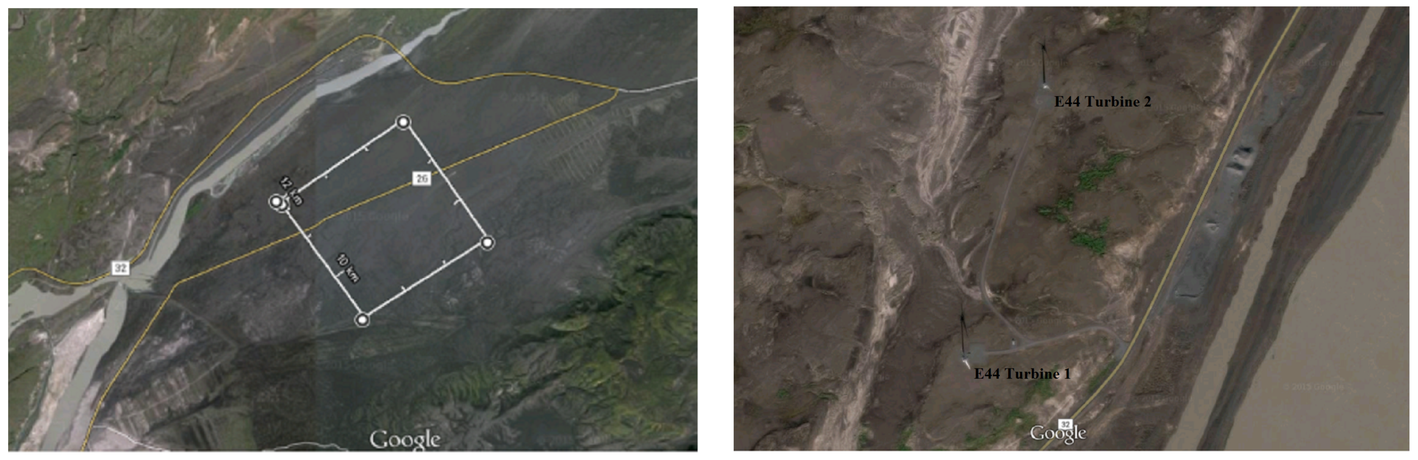
3.1. Site
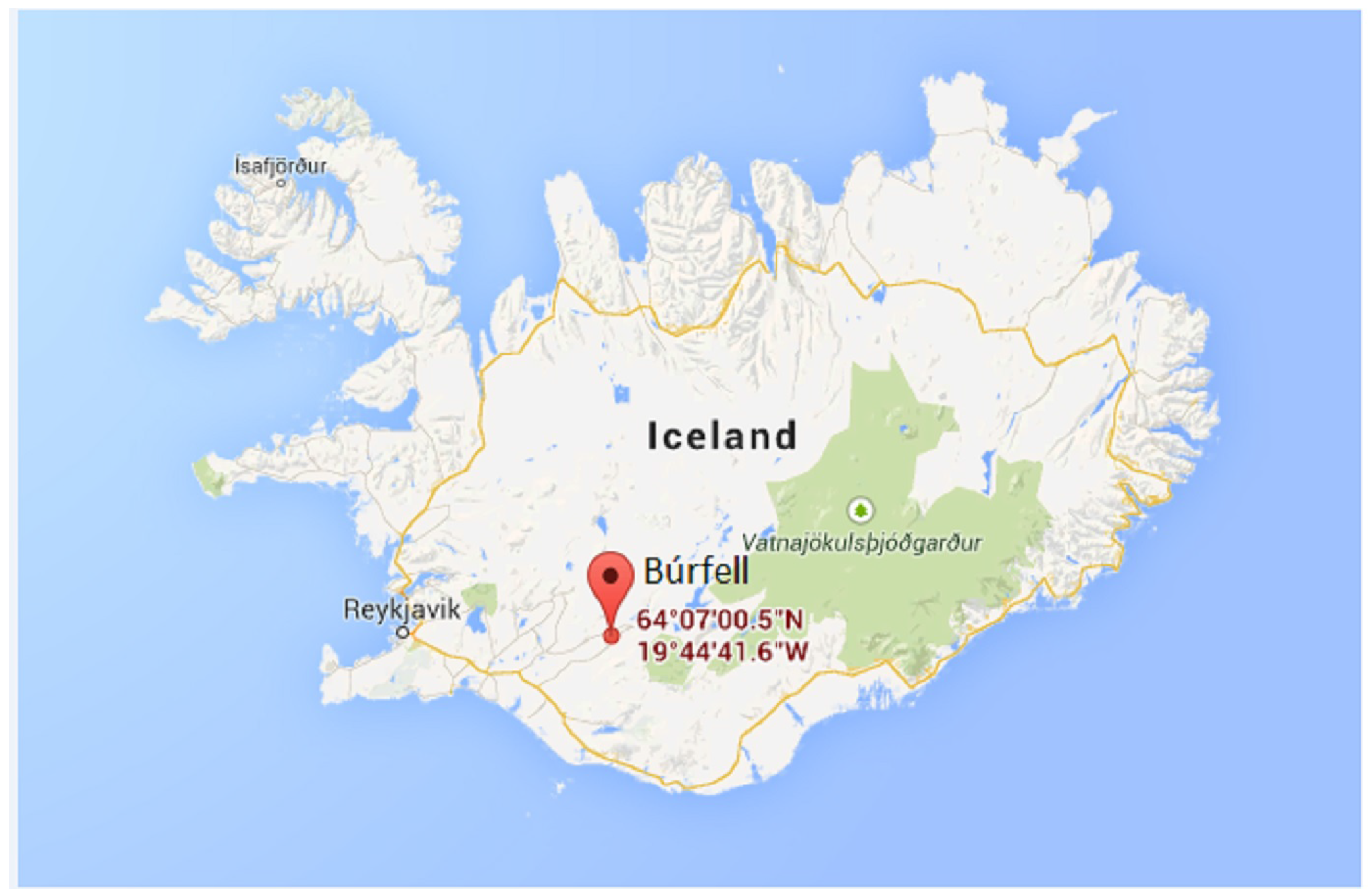
The site selected, Búrfell, is located in the south of Iceland; see
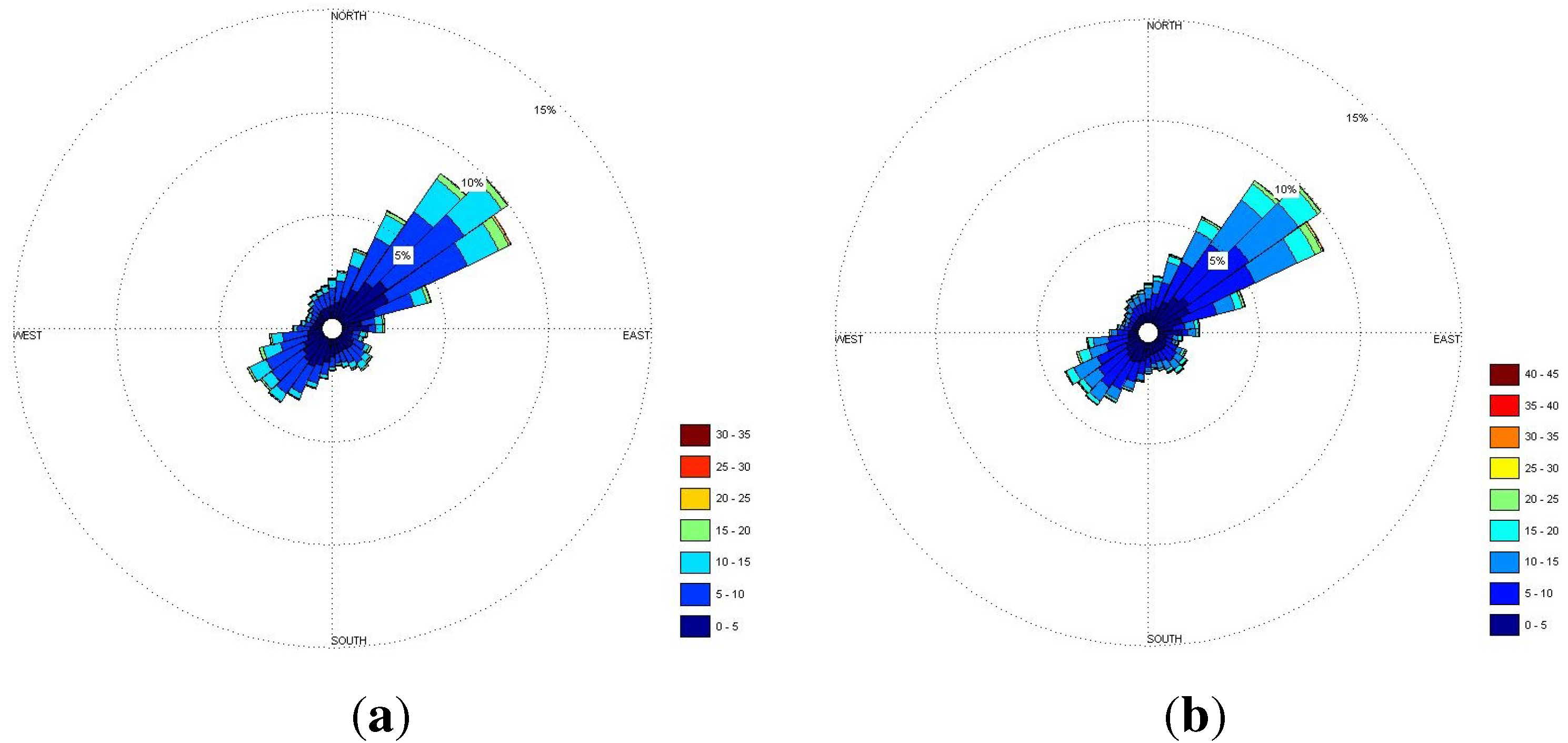
Figure 1. The site has two wind turbines of the type Enercon E44 900 kW installed. The anemometers of the wind turbines mounted on the nacelles were used to gather wind data at a 55-m height. The wind rose diagrams in
Figure 2 show measured wind at the site (10- and 55-m height), the wind direction and the relative frequency of the wind (a color scale is used to show the wind speed). The wind rose diagram was generated using computer code in MATLAB developed by Marta-Almeida [
66].
Wind speed data were gathered from two sources: the Icelandic Meteorological Office and Landsvirkjun, the national power company of Iceland. The data from the Icelandic Meteorological Office were wind speed data measured at a 10-m height in the years 2004–2013; the measurements were performed by using a “Young Wind Monitor”, which is a wind speed sensor with a four-blade helicoid propeller. The data from Landsvirkjun contained one-year (February 2013–February 2014) wind speed data measured at a 55-m height (10-min average values); see
Figure 3 for detailed information. The power law was used to extrapolate the data from a 10-m height to the desired wind power production at a 55-m height when comparing the actual and to 78 m when calculating LCOE.
Figure 1.
Location of Búrfell in the south Iceland [
67].
Figure 1.
Location of Búrfell in the south Iceland [
67].
Figure 2.
Wind rose diagrams of the measured 10-m wind (a) and 55-m wind (b).
Figure 2.
Wind rose diagrams of the measured 10-m wind (a) and 55-m wind (b).
From
Figure 2, it can be concluded that the prevailing wind direction at the site is from northeast (NE). Noticeably, there is also some wind coming from the southwest (SW) direction, but NE appears to be the dominating direction.
The statistics of the wind at site are presented in
Table 1.
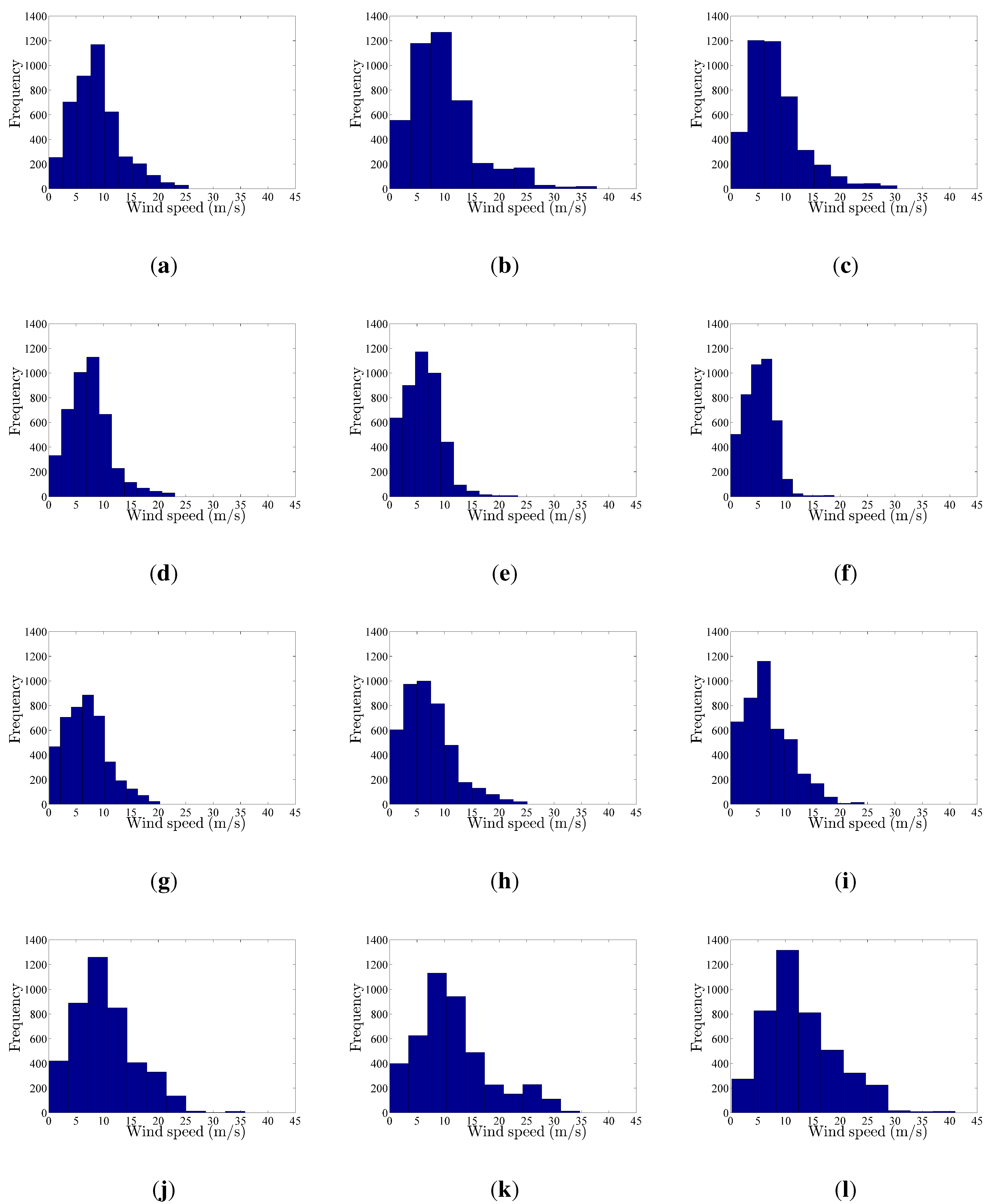
The histogram of wind speed data measured at a 55-m height for each month from February 2013–January 2014 is presented in
Figure 3.
Table 1.
Measured wind speed data at Búrfell.
Table 1.
Measured wind speed data at Búrfell.
| Búrfell | Mean | Median | Standard deviation (SD) |
|---|
| Measured wind speed (m/s) at 10 m | 6.98 | 6.59 | 4.14 |
| Measured wind speed (m/s) at 55 m | 8.73 | 8.24 | 5.18 |
Figure 3.
Histograms of wind speed data measured at a 55-m height for each month from February 2013–January 2014. (a) February; (b) March; (c) April; (d) May; (e) June; (f) July; (g) August; (h) September; (i) October; (j) November; (k) December; and (l) January.
Figure 3.
Histograms of wind speed data measured at a 55-m height for each month from February 2013–January 2014. (a) February; (b) March; (c) April; (d) May; (e) June; (f) July; (g) August; (h) September; (i) October; (j) November; (k) December; and (l) January.
3.2. Wind Farm Layout
The wind farm is assumed to have an irregular array layout, one row offset behind the other. This type of layout is presented in González-Longatt
et al.’s [
68] research on the wake effect in wind farm performances. The layout array has four rotor diameters (RD) between towers and a seven RD spacing between rows; the array should face perpendicular to the prevailing wind direction, and it is designed to minimize wake effects on AEP. This kind of layout provides a long-term wake loss of 0.52 % on average according to González-Longatt
et al.’s [
68] research, which is quite low compared to the traditional rectangular array layout setup. González-Longatt
et al.’s [
68] research states that this estimation of wake loss can be used as a rule of thumb in generic assessments when full-blown wake loss assessment is not performed. However, since wake loss assessment has not been performed on this specific site, a sensitivity analysis on wake loss effects on the final results (LCOE) is presented in the Results Section.
In addition, the Enercon manufacturer recommends in general for wind farm layouts that Enercon turbines should be placed at a minimum of five RD in the prevailing wind direction and at least three RD in directions of less distinct wind. The layout proposed in this study is constructed with arrays of turbines with seven RD between them in the prevailing wind direction and four RD in the less distinct wind direction [
69].
3.3. Wind Turbines and Space Requirements
The wind turbine selected for the LCOE scenario was the Enercon E82 3000-kW turbine; the selection was made based on the fact that two smaller test turbines of type Enercon E44 900 kW are located at the site and have shown promising performance under the conditions at the site; see
Figure 4 for reference. The stats table for the Enercon E82 and the Enercon E44 is presented in
Table 2.
Table 2.
Stats table over the Enercon E44 and E82 wind turbines. IEC: International Electrotechnical Commission.
Table 2.
Stats table over the Enercon E44 and E82 wind turbines. IEC: International Electrotechnical Commission.
| Wind turbine | Rotor diameter (RD) (m) | Hub height (m) | Swept area (m) | Wind class |
|---|
| E44 900 kW | 44 | 55 | 1521 | IEC IA |
| E82 3000 kW | 82 | 78 | 5281 | IEC IA |
| |
The E82 has a rotor diameter of 82 m, and according to the layout described in the section above, the total area required would be approximately 4.23 km
.
Figure 5 shows the space available at the site; for reference, the box marked in the figure represents approximately 9 km
. Note that the space available is not only restricted to the marked box. Therefore, it is concluded that space is not an issue for this wind farm project.
Figure 5 also shows the layout of the existing E44 test turbines.
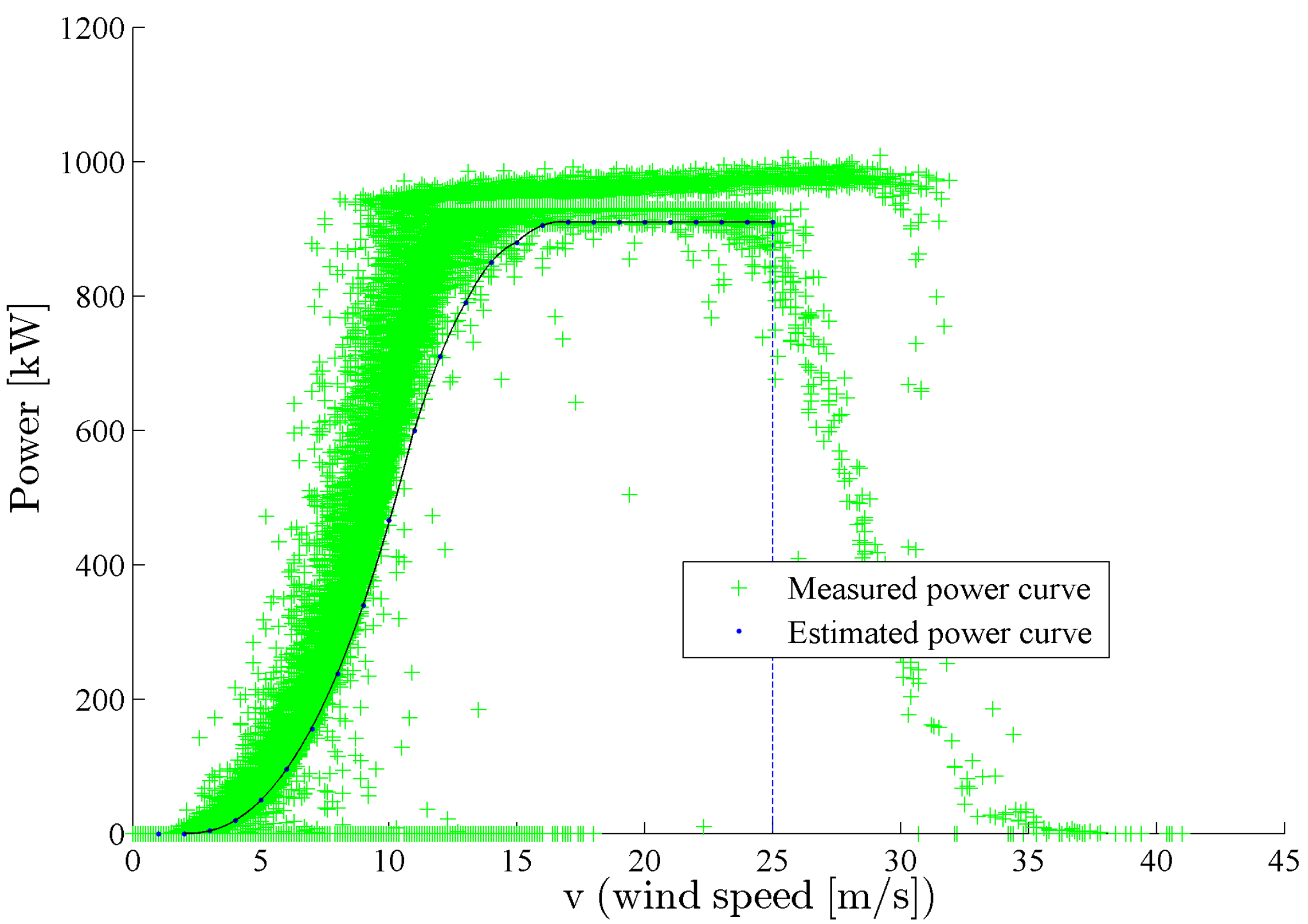
Power curves published by Enercon were used in calculations for the power output given by the Enercon E44 and E82. The E44 power curve was compared to real-time data of the actual power output by the E44 on site. This revealed that the published power curve from Enercon gives a conservative estimate of actual power output at this specific site; see
Figure 4. For this site, it was thus concluded that mechanical losses in power production are included in the power curve estimate given by the manufacturer.
Figure 4.
Measured power curve vs. estimated curve for the E44 turbine.
Figure 4.
Measured power curve vs. estimated curve for the E44 turbine.
Figure 5.
The space available at the Búrfell site is shown on the left and the layout of the E44 test turbines on the right [
67].
Figure 5.
The space available at the Búrfell site is shown on the left and the layout of the E44 test turbines on the right [
67].
Availability data for the two E44 test turbines are presented in
Table 3 and were recorded at their first year in production. The availability of wind turbines is defined as the time that the wind turbine is available for power production, sometimes also called up-time.
Table 3.
Measured availability for both E44 900-kW wind turbines at Búrfell.
Table 3.
Measured availability for both E44 900-kW wind turbines at Búrfell.
| Búrfell | E44 Turbine 1 | E44 Turbine 2 |
|---|
| Availability (%) | 98.65 | 89.16 |
The E44 test turbines experienced 6.095% availability loss on average. Total loss of the wind farm will thus be 6.615%, including wake and availability loss. Assumptions combined with the experienced data of total possible loss in wind energy generation will be used when estimating the LCOE of a future scenario wind power generation system at the site.
4. Results
In this section, the wind energy production potential at Búrfell is assessed. The power law is used to calculate the wind shear exponent (α), which can be used to extrapolate the measured data to the hub height of the E44 test turbines and the E82 turbine selected for the potential wind farm scenario at Búrfell. The modified Weibull simulation method is used to simulate the wind speed distribution at Búrfell. Power law extrapolated data are used as input. The results from the simulation used along side the E44 power curve to calculate the simulated AEP are compared to the measured AEP of the E44 turbine. The comparison showed that the modified Weibull simulation model was applicable for simulating the AEP at the site. Based on that knowledge, the modified Weibull simulation model was used to simulate the AEP for a 99-MW wind farm with 33 E82 3000 kW wind turbines. The power law was used to extrapolate measured data to the desired hub height (78 m) of the E82 turbine. Numerical results and figures from the calculations are presented in this section.
4.1. Extrapolated Data Compared to Measured Data
As a measure of the accuracy of the power law extrapolation, the wind shear factor, calculated as shown in
Table 4, was used to extrapolate wind data from Búrfell measured at a 10-m height to a 55-m height and then compared to measured data at a 55-m height. The data used for the comparison are from February 2013–January 2014. A quantile-quantile plot was made to determine whether the wind speed extrapolated to a 55-m height came from the same distribution as measured wind speed at a 55-m height. If they do, the plotted points will be linear; the red reference line is drawn on the plot to help judge linearity. The plot was conducted using the built-in MATLAB function QQ-plot. It can be seen in
Figure 6, where an example of measured wind speed at a 55-m height
vs. extrapolated wind speed using the power law is shown, that the points appear to be approximately linear up to a wind speed above 15 m/s. At a wind speed above 15 m/s, the power law appears to underestimate the wind speed; this will be noted in power production forecasting [
70].
Table 4.
The median wind shear factor α and its 95% bootstrap confidence interval.
Table 4.
The median wind shear factor α and its 95% bootstrap confidence interval.
| α | Lower α Value | Upper α Value |
|---|
| 0.1309 | 0.1192 | 0.1399 |
| |
The wind shear exponent α was derived from Equation (
1) as a function of
and
and calculated for each data point. The resulting sample of α values contained a few large and small values, some of which reached up to plus four and minus three. Hence, it was decided to use the sample median value for the wind shear exponent rather than the sample mean, as it might be sensitive to extremely small and large values. The calculated median wind shear exponent α is 0.1309. The exponent and the 95% bootstrap confidence interval are shown in
Table 4. The built-in MATLAB function BOOTCI was used to compute the confidence interval. The median wind shear factor α can be used to extrapolate the wind speed data measured at a 10-m height up to the desired wind turbine height. This verifies that the power law is applicable at Búrfell; the deviation in the power law approximation, however, is noted at wind speeds above 15 m/s. Note that the mean wind speed at Búrfell is 8.73 m/s, which means that the power law can extrapolate most of the wind with high accuracy.
Figure 6.
QQ-plot of measured data at 55 m vs. extrapolated data to a 55-m height.
Figure 6.
QQ-plot of measured data at 55 m vs. extrapolated data to a 55-m height.
4.2. Weibull Simulation of Wind at Búrfell
Weibull-distributed wind years were simulated according to the statistics in
Table 5. The built-in function WBLRND in MATLAB was used to generate each simulated year; this function takes in the Weibull parameters from each sector and the amount of data desired to generate in each sector. All sectors are consequently added together, generating one simulated year; this was repeated 2000 times in the simulation.
The number of generated points in each sector is decided by the observed frequency of data from each sector. The underlying proportion of data points within the sectors is assumed to be fixed, but the frequency of data points in the sectors is however not the same from year to year. The frequency of data points within the sectors is allowed to vary according to the multinomial distribution. The frequency ratio in
Table 5 gives estimates of the proportions of data points in the sectors. The multinomial distribution generates years with the variate number of data points in each sector with a total number of data points equal to 52,560, as that is the number of data points in one measured wind speed year (10-min average data).
The results of the modified Weibull fit parameters within directional sectors are presented in
Table 5. The NE sector is the dominant wind direction at Búrfell; this can also be seen clearly in
Figure 2.
Table 5.
Stats table of the modified Weibull fit for wind speed at Búrfell at a 55-m height.
Table 5.
Stats table of the modified Weibull fit for wind speed at Búrfell at a 55-m height.
| Sector | k (m/s) | Mean wind speed (m/s) | A | Frequency (%) | Zero values (%) |
|---|
| N | 9.27 | 7.72 | 1.47 | 9.07 | 8.25 |
| NE | 10.72 | 9.53 | 1.92 | 36.17 | 0.11 |
| E | 9.84 | 8.84 | 1.66 | 9.46 | 0.14 |
| SE | 9.15 | 8.27 | 1.53 | 4.92 | 0.20 |
| S | 10.27 | 9.19 | 1.72 | 8.16 | 0.15 |
| SW | 9.41 | 8.37 | 1.93 | 16.52 | 0.07 |
| W | 7.47 | 6.75 | 1.46 | 7.77 | 0.15 |
| NW | 9.55 | 8.60 | 1.55 | 7.93 | 0.23 |
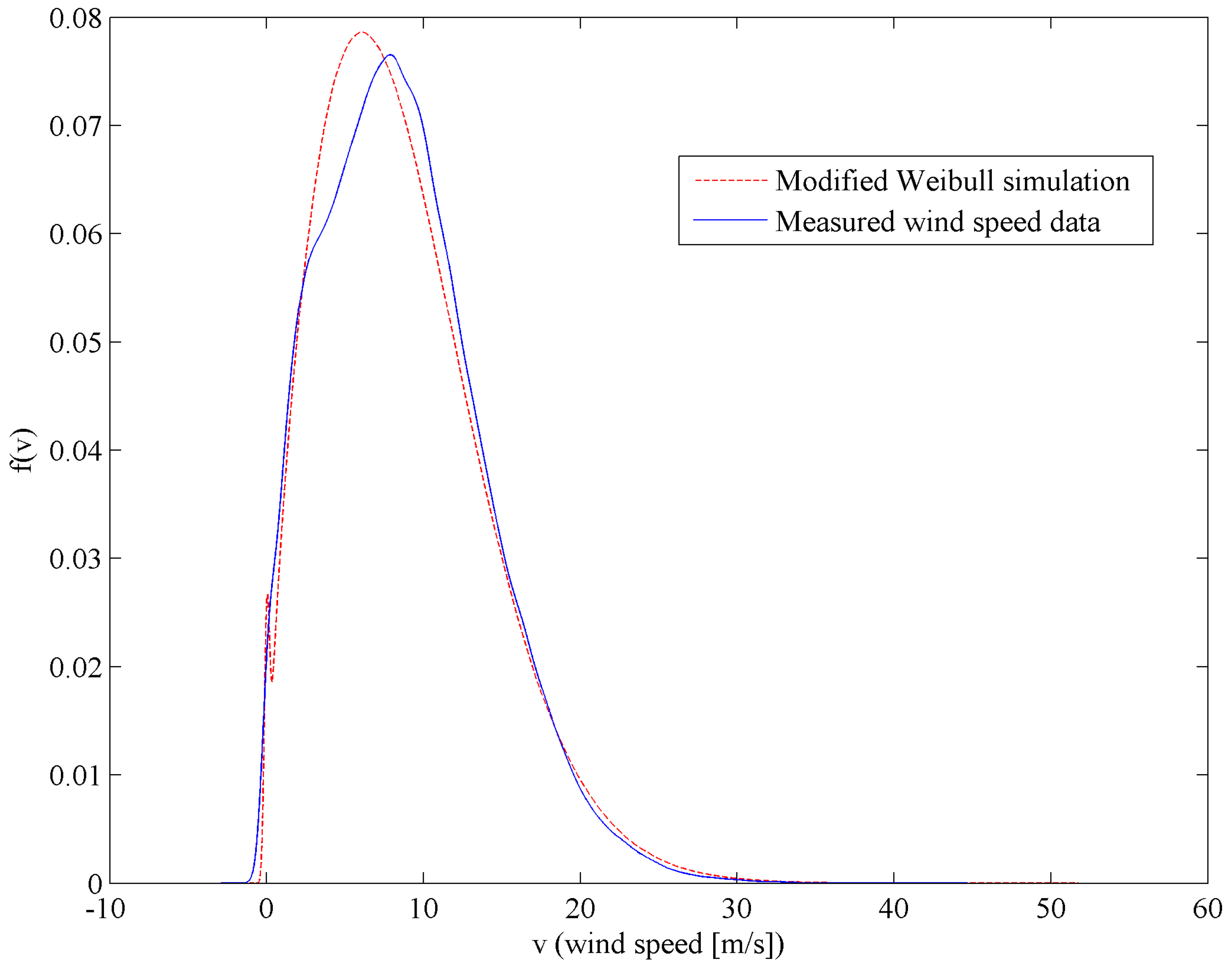
The results and comparison of the modified Weibull fit simulation
vs. measured wind speed at Búrfell are presented in
Figure 7 and
Table 6. The modified Weibull fitted wind speed distribution is very comparable to the measured data; there is however a slight deviation at the top of the curve. The mean wind speed for the modified Weibull simulation and measured data at Búrfell is very similar, and the same goes for the SD, as can be seen from
Table 6.
Figure 7.
Probability density function (PDF) of the modified Weibull simulated wind speed at Búrfell.
Figure 7.
Probability density function (PDF) of the modified Weibull simulated wind speed at Búrfell.
Table 6.
Measured wind speed data vs. Weibull fit for wind speed at Búrfell at a 55-m height.
Table 6.
Measured wind speed data vs. Weibull fit for wind speed at Búrfell at a 55-m height.
| Búrfell | Mean (m/s) | Median (m/s) | SD (m/s) |
|---|
| Weibull fit | 8.47 | 7.05 | 6.32 |
| Modified Weibull fit | 8.70 | 7.93 | 5.29 |
| Measured wind speed | 8.73 | 8.24 | 5.18 |
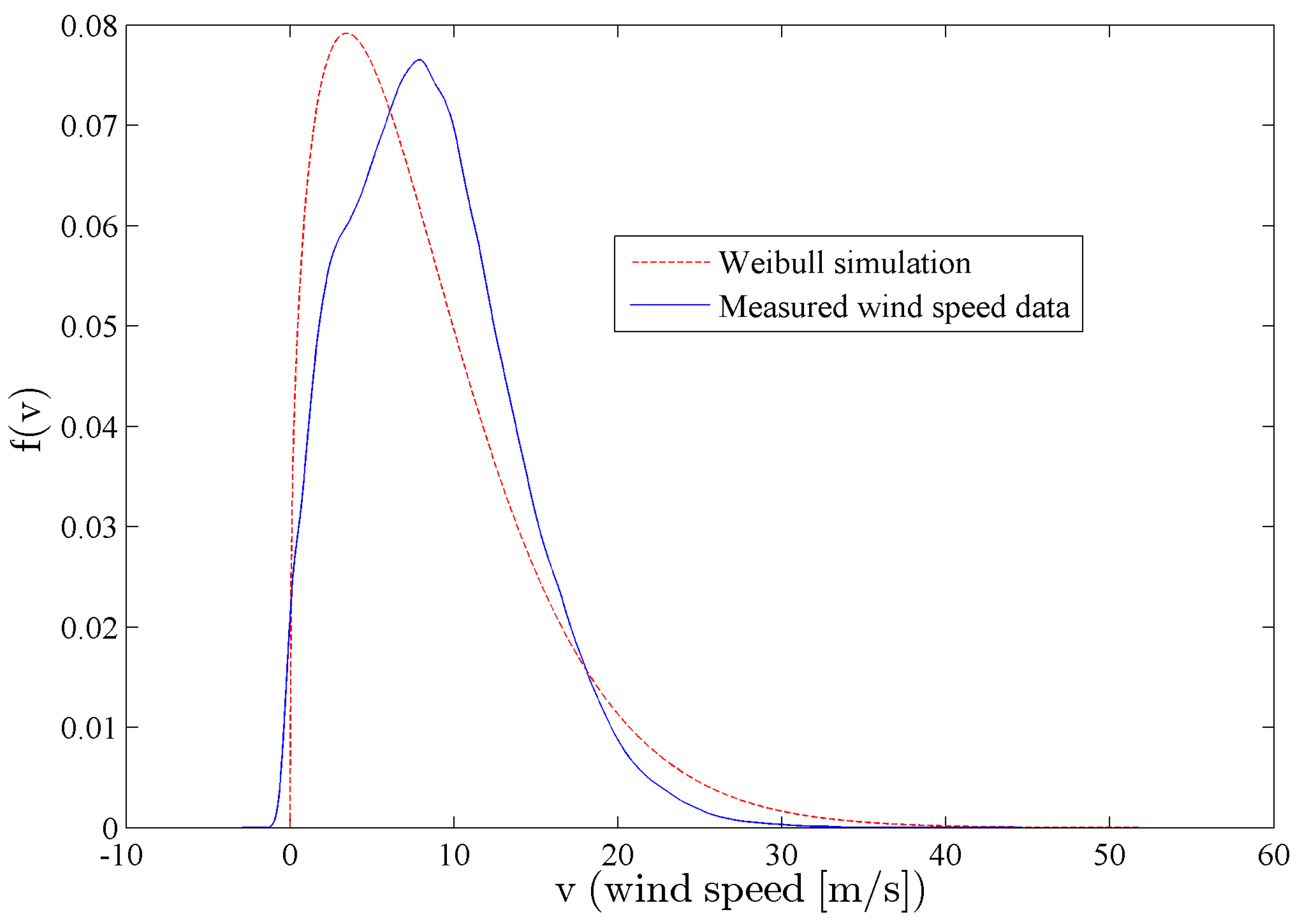
For a comparison,
Figure 8 shows the Weibull distribution fitted to data without modifications, that is fitting one
A and
k parameter to all data and not taking the zeros into account.
Figure 8.
PDF of the Weibull distribution and measured wind speed data.
Figure 8.
PDF of the Weibull distribution and measured wind speed data.
It can be seen that the Weibull fit is skewed to the left. This is not surprising, since it is unreasonable to fit one Weibull distribution to all data, because of the fact that wind distribution is different between yearly weather seasons [
64].
4.3. Comparison of Simulated Annual Energy Production (AEP) vs. Measured AEP
The AEP for the E44 900-kW turbine at Búrfell was calculated for each simulated year
t for the Weibull simulation. The E44 wind turbine is the same as the two installed test turbines at Búrfell. Thus, the calculated results can be compared to the measured AEP data, verifying the simulation result. Measured power production output data from the two 900-kW test turbines at Búrfell is available from the end of January 2013 until the present. The AEP in MWh of Turbines 1 and 2 from February 2013–January 2014 is presented in
Table 7; the data were provided by Landsvirkjun.
Table 7.
Measured annual energy production (AEP) and capacity factor (CF) for both E44 900-kW wind turbines at Búrfell.
Table 7.
Measured annual energy production (AEP) and capacity factor (CF) for both E44 900-kW wind turbines at Búrfell.
| Búrfell | E44 Turbine 1 | E44 Turbine 2 |
|---|
| AEP (MWh) | 3184.8 | 2939.4 |
| CF (%) | 40.39 | 37.28 |
The difference in the AEP for the two turbines, shown in
Table 7, is due to the different availability between the two turbines. Each turbine experienced different amounts of downtime caused by malfunctioning. Hence, the measured data used for generating
Table 7 have to be scaled up according to the availability data for the two E44 turbines (
Table 3). The scaling makes sure that measured and calculated results are being compared to the same amount of production hours in the year. The scaled data for the measured AEP are presented in
Table 8. This is done because simulated AEP assumes that the wind turbines are producing power throughout every hour of the year.
Table 8.
Scaled measured AEP and CF for both 900-kW wind turbines at Búrfell.
Table 8.
Scaled measured AEP and CF for both 900-kW wind turbines at Búrfell.
| Búrfell | E44 Turbine 1 | E44 Turbine 2 |
|---|
| AEP (MWh) | 3228.24 | 3296.91 |
| CF (%) | 40.94 | 41.8 |
The two E44 turbines are located side by side, and thus, they should produce almost exactly the same amount of energy. After scaling the measured AEP by the availability data for each turbine, the AEP values are very similar.
Table 8 can consequently be used to compare measured
vs. simulated AEP.
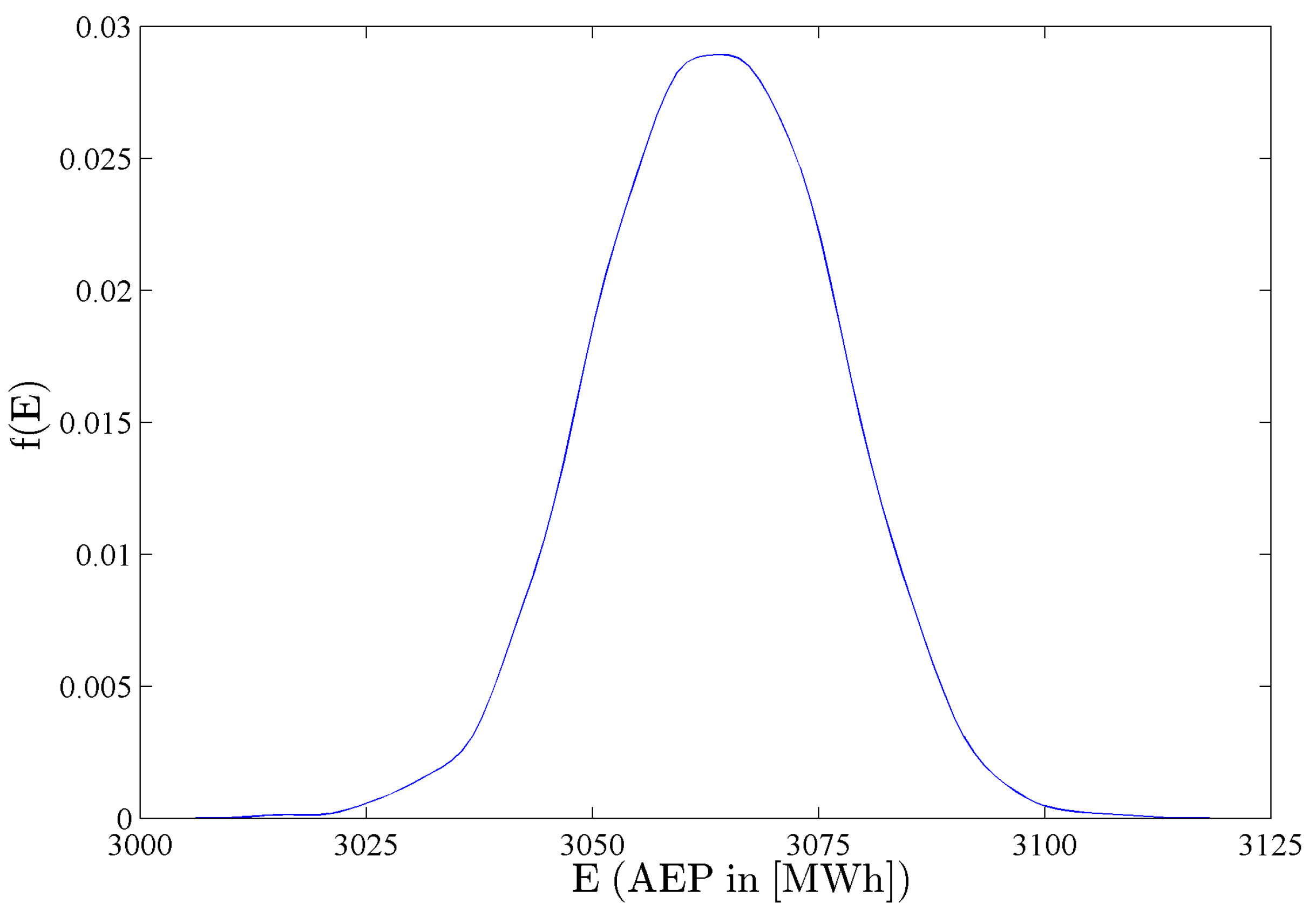
4.3.1. Annual Energy Production (AEP) Calculated from Modified Weibull Simulated Wind Data
For each modified Weibull simulated wind year, the AEP is calculated using Equation (
5). The mean AEP and CF with a 95% prediction interval are presented in
Table 9 and
Figure 9. Notice that the prediction interval for the modified Weibull simulated AEP is quite narrow. This is also evident in
Figure 9, which shows the probability density of the simulated AEP. The Weibull distribution simulates wind speed values independently, meaning that one simulated 10-min average wind speed is not correlated to the 10-min average wind speed of the consecutive 10-min period. This type of simulation gives a quite good estimate of the mean, but it, however, does not manage to replicate the variation in wind between years, hence the narrow 95% prediction interval.
Table 9.
Modified Weibull simulated AEP for E44 900-kW wind turbine (55-m hub height).
Table 9.
Modified Weibull simulated AEP for E44 900-kW wind turbine (55-m hub height).
| Búrfell | Mean | 95% Prediction interval |
|---|
| AEP (MWh) | 3063.67 | 3042.42 | 3084.46 |
| CF (%) | 38.85 | 38.58 | 39.12 |
The estimated mean CF is 38.85% at Búrfell based on the modified Weibull wind simulation. The 95% prediction interval is from 38.58%–39.12%. This prediction interval does not include the measured CF at Búrfell, which is due to the fact that the Weibull simulation does not capture the true wind process perfectly, but it is sufficiently close and gives a conservative estimate of the CF,
i.e., an estimate that is below the measured CF. This result confirms that the modified Weibull simulation model presented is sufficiently accurate to use when performing an LCOE analysis for a wind power generation system at Búrfell. This conclusion is made based on a comparison of simulated AEP compared to measured AEP at the site. Note that when comparing measured AEP to simulated AEP, wake loss is disregarded for comparison purposes. The two test wind turbines are placed in a straight line perpendicular to the prevailing wind direction, which minimizes wake loss effects [
68]. The AEP of the test turbines are on-site measurements; thus, it can be stated that wake loss is already included in the measured value. Availability loss is included, but scaled accordingly for comparison. LCOE analysis takes into account the total losses of the power generation system according to the data and assumptions made in
Section 3.3.
Figure 9.
PDF of Weibull simulated AEP for the E44 wind turbine at Búrfell.
Figure 9.
PDF of Weibull simulated AEP for the E44 wind turbine at Búrfell.
4.4. Economical Analysis
Cost data were gathered from Landsvirkjun and from the literature from international constitutions, such as International Renewable Energy Agency (IRENA) and the European Wind Energy Association (EWEA). Experience data from the two test turbines tested at Búrfell are available through Landsvirkjun; these data are used in combination when assessing the LCOE at Búrfell.
4.5. Levelized Cost of Energy (LCOE) Estimation
The LCOE for Búrfell was assessed using Equation (
7), the inputs in the equation were simulated AEP from the Weibull simulation. Cost data were acquired from Landsvirkjun and IRENA. The energy production lifetime of the project was assumed to be 25 years. CAPEX is calculated with the value of 2229 USD/kW, and the OPEX is set to 0.015 USD/kWh, according to data from Landsvirkjun gathered from experience when building the two E44 test turbines. CAPEX is assumed to be invested in 2014, and one year is assumed for building the wind farm; the first energy production year is thus set to the year 2016. OPEX cost was inflated yearly with fixed 2.20% inflation [
71], and WACC was set to 10% in the general LCOE calculation for European comparison, but also 6%, which Landsvirkjun uses. The inflation rate estimate was acquired from Hagstofa Íslands (Statistics Iceland). The capacity of the wind farm for the LCOE estimation scenario was set to 99 MW or 33 Enercon E82 3000-kW turbines, this scenario was considered reasonable at the Búrfell site according to consulting advice from Landsvirkjun. The Weibull simulated AEP for one E82 turbine is presented in
Table 10, and the net gross AEP, including losses, is presented for the wind farm at Búrfell in
Table 10. The results of the LCOE estimation are presented in
Table 10 [
70].
Table 10.
AEP and levelized cost of energy (LCOE) results. WACC: weighted average cost of capital.
Table 10.
AEP and levelized cost of energy (LCOE) results. WACC: weighted average cost of capital.
| | No. of E82’s | WACC | Mean | 95% Prediction interval |
|---|
| AEP (GWh) | 1 | - | 10.03 | 9.96 | 10.08 |
| CF (%) | 1 | - | 38.15 | 37.90 | 38.38 |
| Net gross AEP (GWh) | 33 | - | 309.01 | 306.97 | 310.80 |
| LCOE (USD/kWh) | 33 | 10% | 0.0873 | 0.0869 | 0.0878 |
| LCOE (USD/kWh) | 33 | 6% | 0.0703 | 0.0700 | 0.0706 |
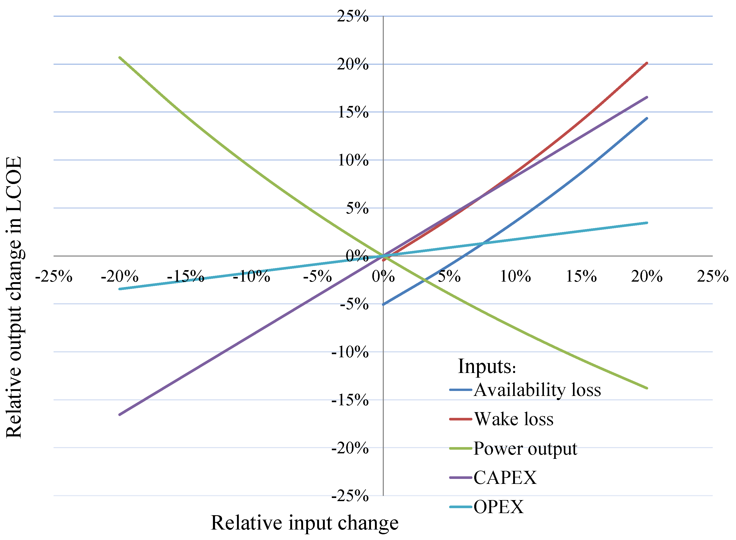
Sensitivity analysis revealed that calculated mean LCOE (10% WACC) is most affected by actual power output; this is not considered surprising for the LCOE of a wind power generation system. The calculated LCOE is also quite sensitive to increased wake loss effects; this is due to the fact that accurate wake loss assessment is yet to be done at the site and because low wake loss was assumed. If the worst case scenario for wake loss (20% wake loss) is assumed, the LCOE increases by approximately 20%, which results in an estimated LCOE of 0.1047 USD/kWh. This scenario, however, is highly unlikely, but gives an idea of the feasibility of the project. The more likely scenario of the 5% wake loss increase gives an LCOE increase of 3.9%, which is estimated approximately as 0.0907 USD/kWh. The relation between LCOE and the input parameters, such as CAPEX, OPEX and the availability loss, is shown in
Figure 10.
Figure 10.
Sensitivity analysis of input parameters to levelized cost of energy (LCOE) (10% WACC) calculation.
Figure 10.
Sensitivity analysis of input parameters to levelized cost of energy (LCOE) (10% WACC) calculation.
The figure can be used to study the relative percentage change in LCOE when the input parameters change; e.g., if the availability loss is increased by 20%, then the LCOE increase is 14%. The assumed availability loss was 6.095% in the mean LCOE calculation; this can be observed in
Figure 10, where the availability curve crosses the horizontal axis (0% change in the LCOE) at approximately a 6% availability loss. Furthermore, if no availability loss were present, the LCOE would decrease by approximately 5% (where the availability loss curve crosses the vertical axis). The results from the estimated LCOE at Búrfell using a WACC of 10% show that the LCOE for wind energy at Búrfell is low compared to the 2010 LCOE estimation for Europe.
5. Conclusions
This article presents the results of wind energy production potential for a proposed wind generation system at Búrfell, with the capacity of 99 MW using the Enercon E82 3000-kW type of wind turbine. The research was set up with the objective to answer the question: What is the LCOE produced by wind at Búrfell?
To answer this question, the researchers went through several steps. First, the wind speed measurements from a 15-m and a 55-m height were used to verify the power law, and the results showed that it is very accurate up to wind speeds of around 15 m/s. At greater wind speed, the power law underestimates the wind speed at the site. Based on these results, the researchers used the power law to extrapolate the wind data from a 15-m to a 78-m height for the suggested wind farm. Second, the data from the two wind turbines installed at the site were used to verify the AEP calculations. A comparison of calculated AEP and the measured AEP showed that the they are about the same (average unscaled measured AEP at 3044 MWh vs. calculated at 3063 MWh). The results were used to calculate AEP for a wind farm, which consists of 33 units of 3-MW wind turbines. The calculated total AEP was 309.01 GWh.
The wind energy production potential assessment revealed that the estimated CF at Búrfell lies between 37.90% and 38.38%. The power produced on average by the wind turbines at Búrfell is estimated to be 38.15% of their rated power production capabilities. The result was obtained using the E82 3000-kW wind turbine as the reference turbine, and the modified Weibull simulation was used for wind speed simulation. This places the Búrfell site among the highest CF-rated sites in Europe and shows high potential for wind energy production, where the average is found to be around 21%.
This estimated AEP result was used to calculate the LCOE of wind energy at Búrfell. The LCOE of wind energy was estimated to be between 0.087 and 0.088 USD/kWh, assuming 10% WACC. This places wind energy harnessing at Búrfell in the same category as the lowest LCOE for wind energy in Europe. As mentioned earlier, researchers have found the LCOE to lie between 0.08 and 0.14 USD/kWh using 10% WACC. Note that Landsvirkjun uses 6% WACC for their energy projects, which means that the estimated LCOE for Landsvirkjun is lower.


 ,
, 


