
Automated Variable Selection and Shrinkage for Day-Ahead Electricity Price Forecasting


Abstract
:
1. Introduction
- nine variants of three parsimonious autoregressive model structures with exogenous variables (ARX): one originally proposed by Misiorek et al. [19] and later used in a number of EPF studies [13,18,20,21,22,23,24,25,26,27], one which evolved from it during the successful participation of TEAM POLAND in the Global Energy Forecasting Competition 2014 (GEFCom2014; see [28,29,30]) and an extension of the former, which creates a stronger link with yesterday’s prices and additionally considers a second exogenous variable (zonal load or wind power),
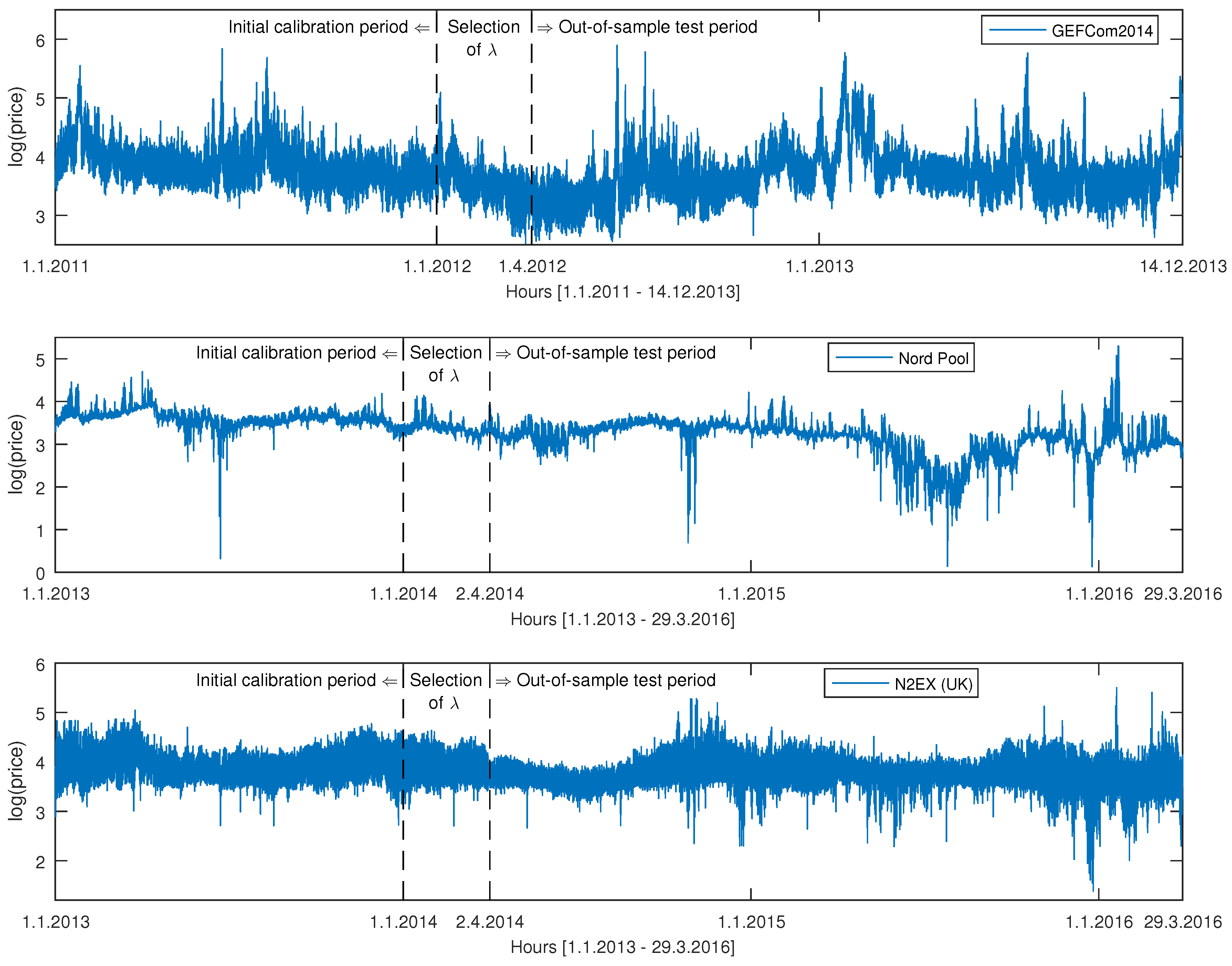
- three two-year long, hourly resolution test periods from three distinct power markets (GEFCom2014, Nord Pool and the U.K.),
- nine variants of five classes of selection and shrinkage procedures: single-step elimination of insignificant predictors (without or with constraints), stepwise regression (with forward selection or backward elimination), ridge regression, lasso and three elastic nets (with , or ),
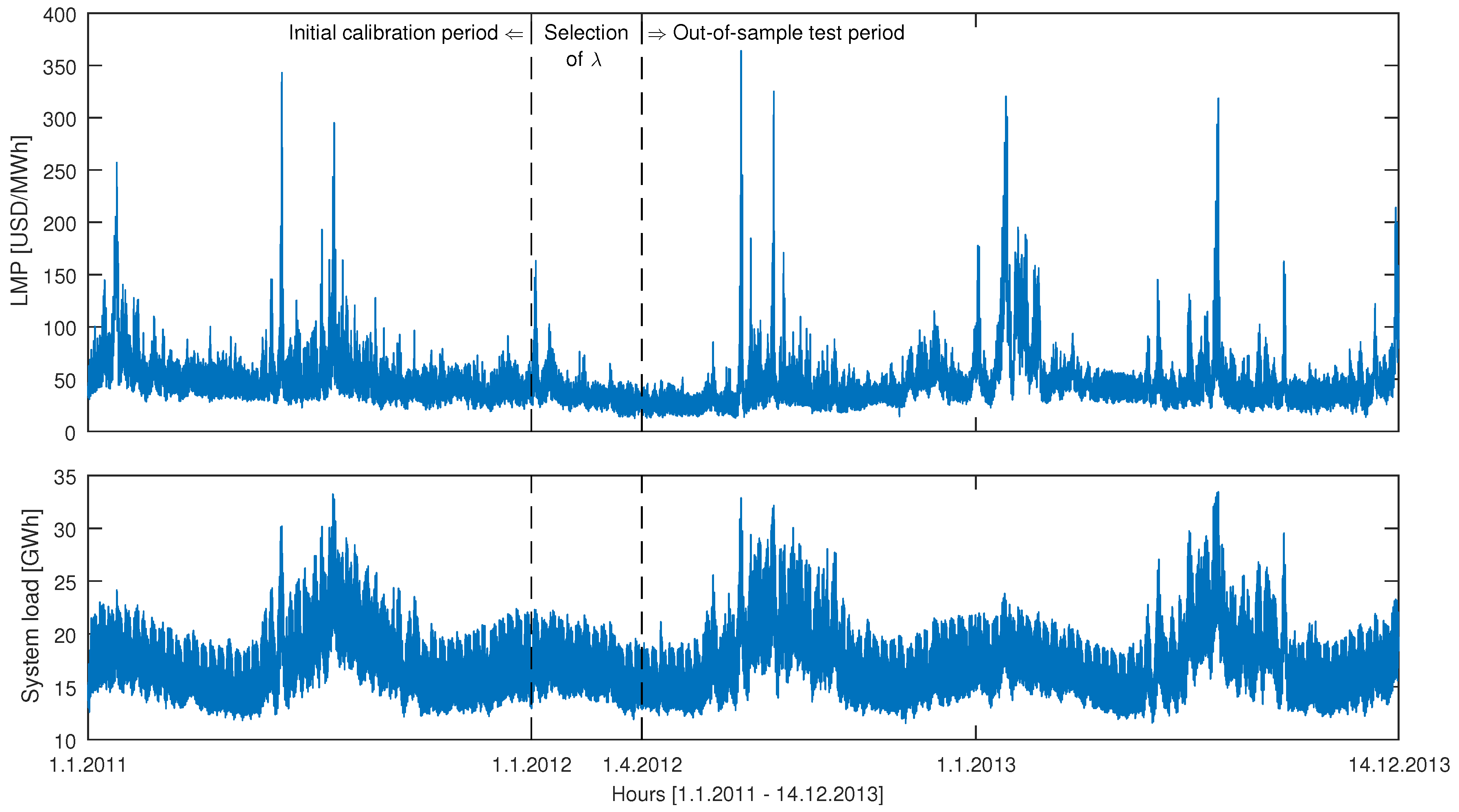
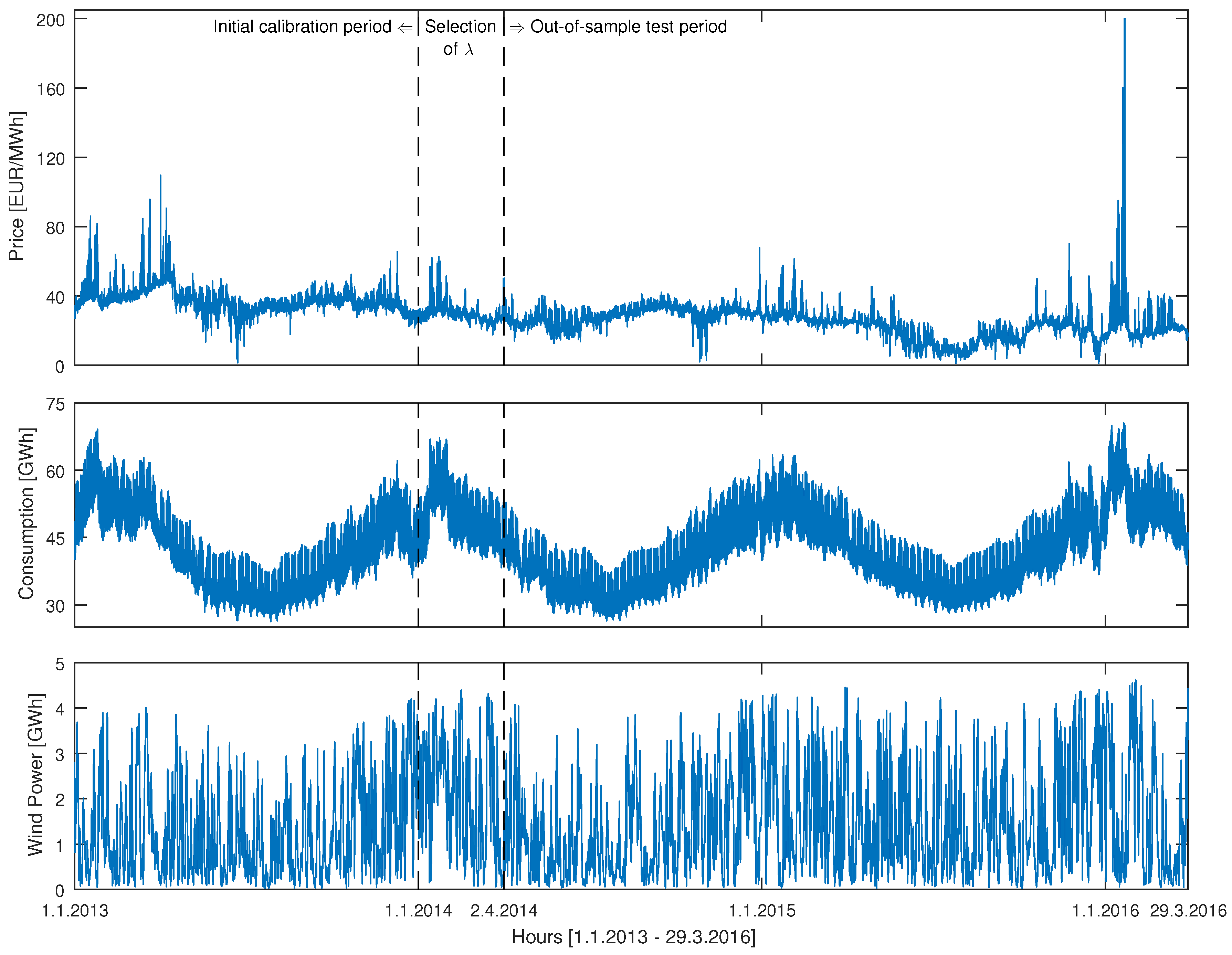
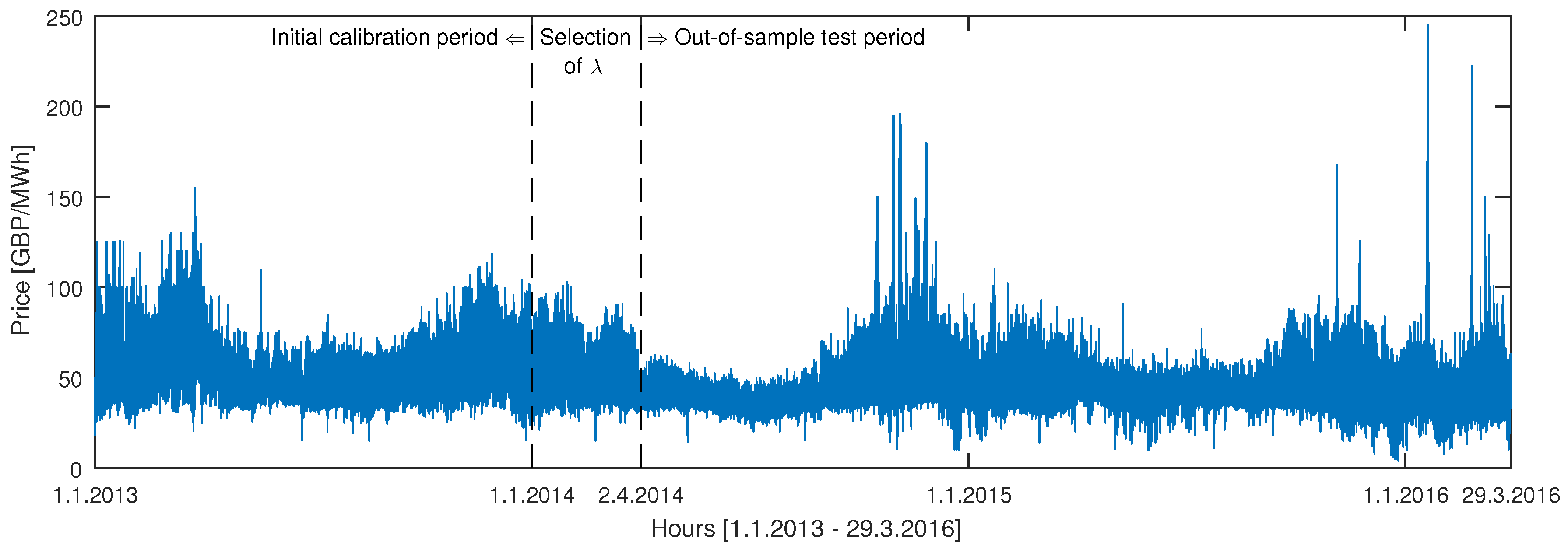
2. Datasets
3. Methodology
3.1. The Naive Benchmark
3.2. Autoregressive Expert Benchmarks
3.3. Full Autoregressive Model
3.4. Selection and Shrinkage Procedures
- variable or subset selection, which involves identifying a subset of predictors that we believe to be influential, then fitting a model using LS on the reduced set of variables,
- shrinkage (also known as regularization), which fits the full model with all predictors using an algorithm that shrinks the estimated coefficients towards zero, which can significantly reduce their variance.
3.4.1. Single-Step Elimination of Insignificant Predictors
3.4.2. Stepwise Regression
3.4.3. Ridge Regression
3.4.4. Lasso and Elastic Nets
- EN25X, EN50X and EN75X when the baseline model is fARX,
- and EN25, EN50 and EN75 when the baseline model is fAR,
4. Empirical Results
4.1. Performance Evaluation in Terms of WMAE
- All models beat the Naive benchmark and, except for the fAR model and the U.K. data, by a large margin. In particular, the improvement from using elastic nets can be as much as 5%! This indicates that they all are highly efficient forecasting tools.
- When we exclude single-step elimination without constraints (ssAR/X) and backward selection (bsAR/X) models, the selection and shrinkage methods generally outperform the expert benchmarks. In particular, the elastic net model with (i.e., closer in terms of α to the lasso than to ridge regression) beats every expert model, except mAR1hm for the U.K. data, where it is second best.
- The latter comment leads us to the next conclusion that adding the price for the last load period of the day, , to the expert models improves their performance greatly. This fact has been recognized in the EPF literature only very recently [18,25,29] and apparently requires more attention. To see this, compare the models with suffix m to those without it. In particular, mAR1hm is the overall best performing model for the U.K. dataset and ARX2hm is the third best model for the Nord Pool dataset.
- Somewhat surprisingly, the full ARX model performs poorly. For the U.K. dataset, it is nearly as bad as the Naive benchmark. In all four cases (three datasets + GEFCom2014 without exogenous variables), it is worse than the overall best model and the best performing elastic net (EN75/X) by at least 1.4%. Given that a 1% improvement in MAPE translates into savings of ca. $1.5 million per year for a typical medium-size utility [2,3], this observation is of high practical value. Yet, from a statistical perspective, this finding is not that surprising. The fARX model has 107 parameters, which have to be calibrated to only 365 observations. Increasing the length of the calibration window should lead to a better performance of the full model.
- Among the selection and shrinkage methods, the lasso and elastic nets tend to outperform single-step elimination (ssAR/X/1), stepwise regression (fsAR/X, bsAR/X) and even ridge regression (Ridge/X). Only for the Nord Pool dataset, the fsARX forward selection model is better than the lasso and two elastic nets.
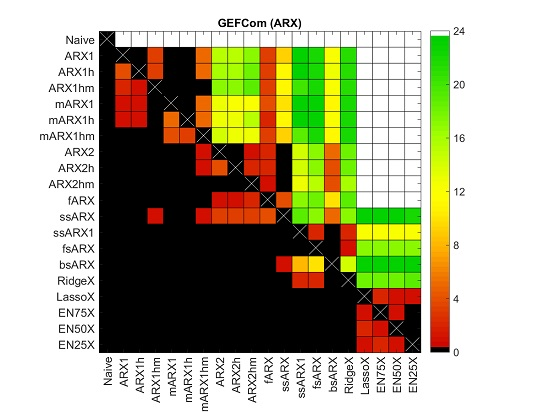
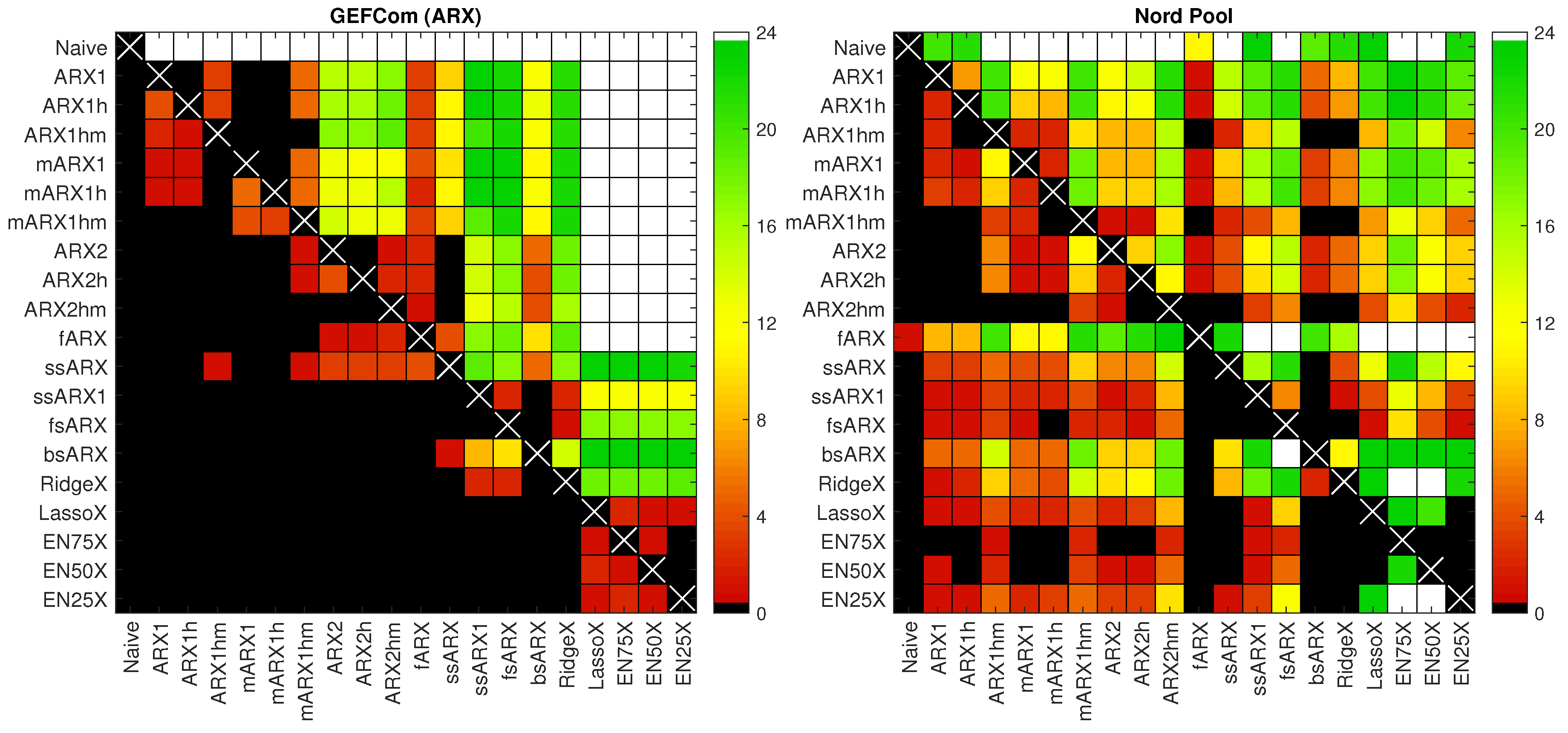
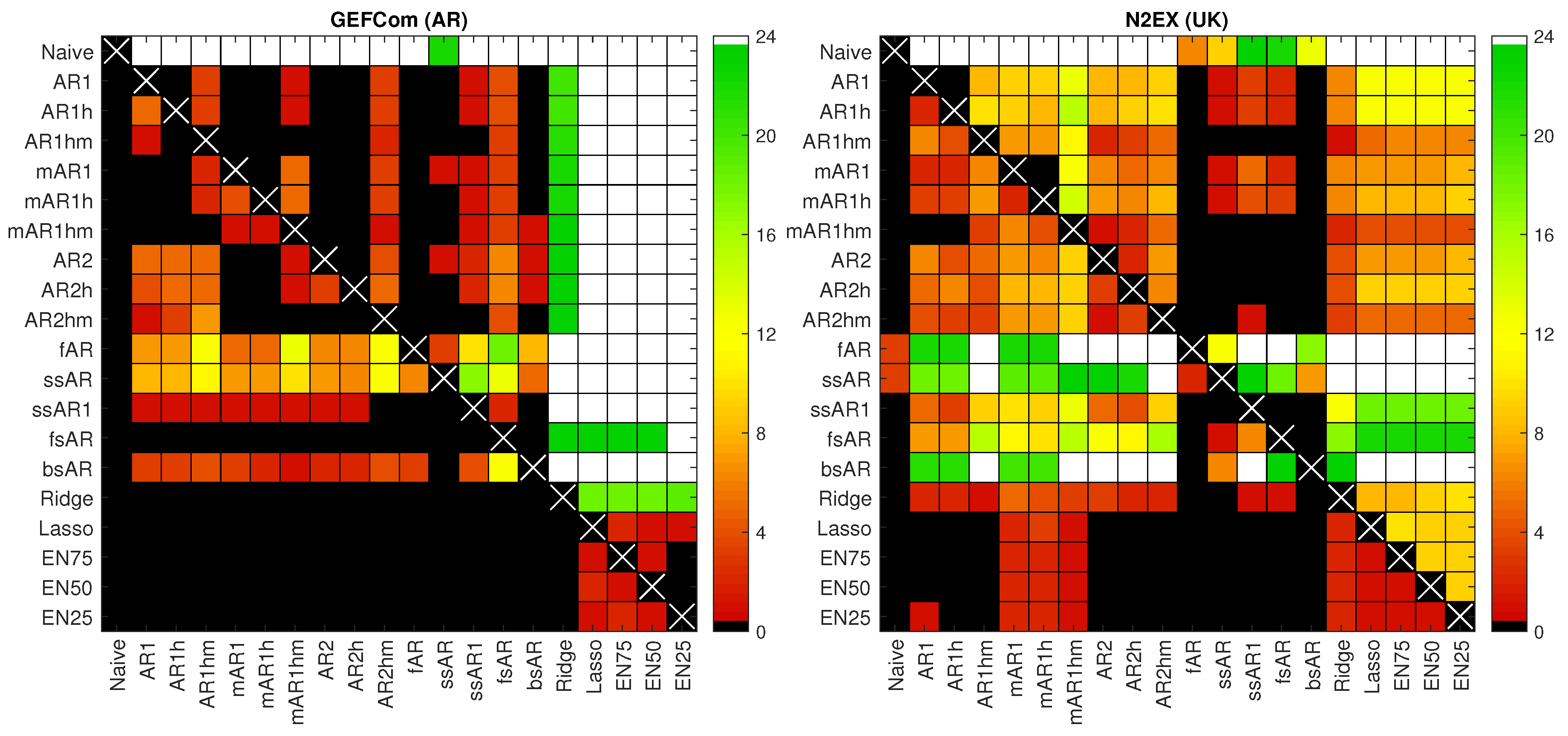
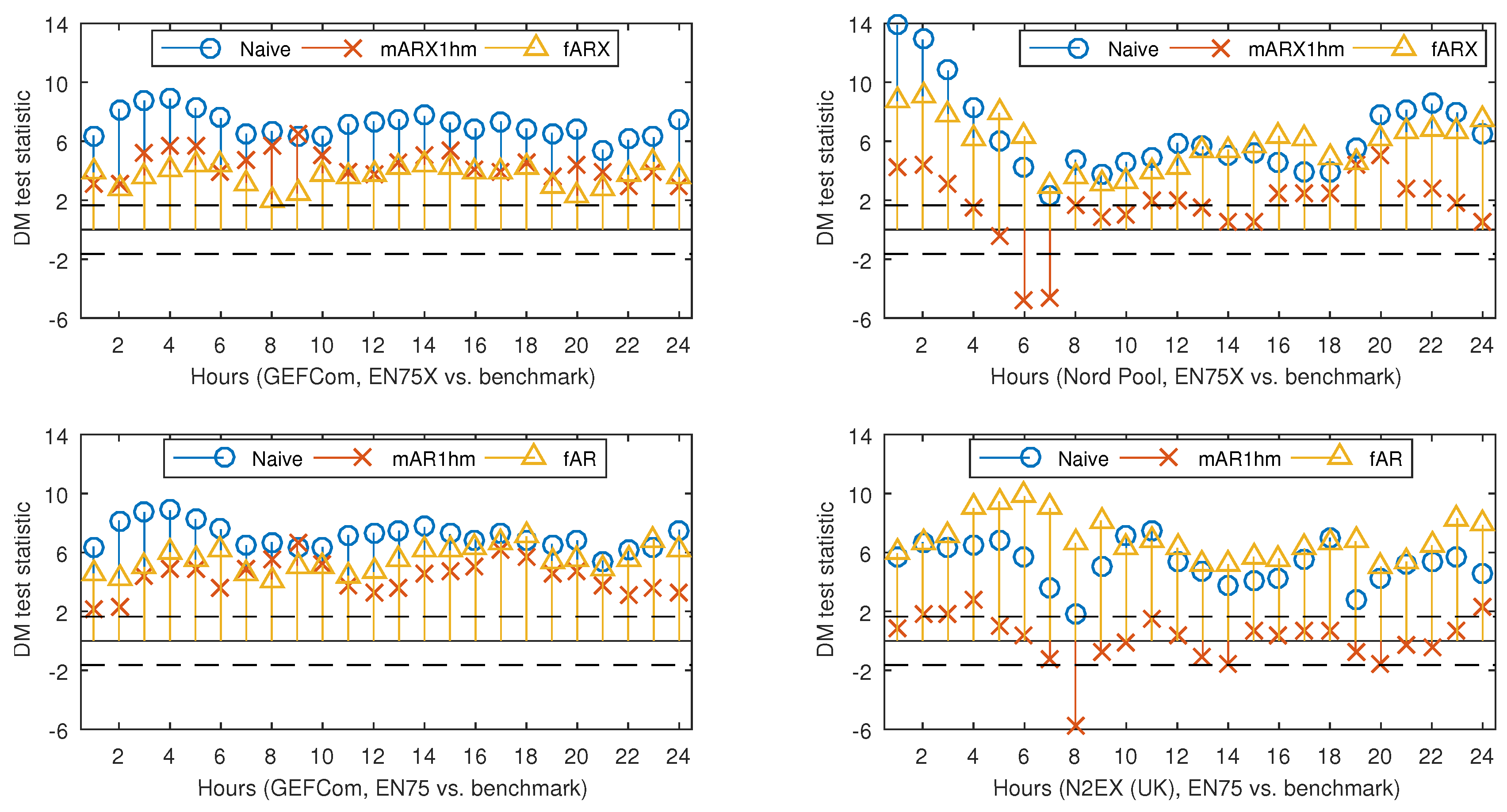
4.2. Diebold–Mariano Tests
4.3. Variable Selection
- There is no single variable that is always used, regardless of the dataset, hour of the day or the day in the out-of-sample test period. The closest to ‘perfection’ is the day-ahead load forecast for the predicted hour, i.e., (see Row 83 in Table 2). Surprisingly, this dependence on the load forecast is stronger than the autoregressive effect (see the next bullet point). This may be a hint that the load-price relationship should be given more attention and that functionals of load-related (or other fundamental) variables should be included in EPF models, like in [10].
- As expected, the price 24 h ago, i.e., , is an influential variable; see the diagonals in Rows 1–24 in both Tables. However, it is not only the same hour a day earlier, but also the neighboring hours. The diagonal is less visible around mid-day, and for Nord Pool, it almost disappears except for the late night hours. The latter may be to some extent due to the importance of wind in this market and the explanatory power of the day-ahead wind prognosis for the predicted hour.
- As recently observed in [18,29], the price for Hour 24, i.e., , is an influential variable. Somewhat surprisingly, sometime between 7–9 a.m. and 9–11 p.m., Hour 22, i.e., , becomes more important. What is more surprising, these late night hours are generally more often selected than the same hour a day ago, i.e., . These observations require more thorough studies. Nevertheless, our limited results suggest that these late hour variables should be taken into account when constructing expert models.
- Clearly, the least important variables for all markets are the daily average prices over the last three days, i.e., for , which are almost never selected. There are some exceptions, though, for the GEFCom2014 dataset and the EN75 model; see Table 3. Of the two other aggregated variables, is slightly more influential than , which contradicts the observations of Misiorek et al. [19] and may suggest its use in expert models instead of the minimum.
- If prices from days or are ever selected, it is only for hours around midnight the day before (i.e., , , ) or similar hours (i.e., the diagonals in Rows 25–48 and 49–72). On the other hand, the same hour one week ago, i.e., , has a high explanatory power (see Row 73 for all datasets), which justifies its use in expert models [18,19,20,21,22,23,30].
- Finally, the weekly dummies (Rows 87–93), the dummy-linked load forecasts (Rows 94–100 in Table 2 only) and the dummy-linked last day’s prices (Rows 101–107) are generally selected for the EN75/X model. This may be an indication that the weekly seasonality requires better modeling than offered by typically-used expert models.
5. Conclusions
Acknowledgments
Author Contributions
Conflicts of Interest
References
- Weron, R. Electricity price forecasting: A review of the state-of-the-art with a look into the future. Int. J. Forecast. 2014, 30, 1030–1081. [Google Scholar]
- Zareipour, H.; Canizares, C.A.; Bhattacharya, K. Economic impact of electricity market price forecasting errors: A demand-side analysis. IEEE Trans. Power Syst. 2010, 25, 254–262. [Google Scholar] [CrossRef]
- Hong, T. Crystal Ball Lessons in Predictive Analytics. EnergyBiz Mag. 2015, 35–37. [Google Scholar]
- Amjady, N.; Keynia, F. Day-ahead price forecasting of electricity markets by mutual information technique and cascaded neuro-evolutionary algorithm. IEEE Trans. Power Syst. 2009, 24, 306–318. [Google Scholar] [CrossRef]
- Gianfreda, A.; Grossi, L. Forecasting Italian electricity zonal prices with exogenous variables. Energy Econ. 2012, 34, 2228–2239. [Google Scholar] [CrossRef] [Green Version]
- Maciejowska, K. Fundamental and speculative shocks, what drives electricity prices? In Proceedings of the 11th International Conference on the European Energy Market (EEM14), Kraków, Poland, 28–30 May 2014. [CrossRef]
- Ludwig, N.; Feuerriegel, S.; Neumann, D. Putting Big Data analytics to work: Feature selection for forecasting electricity prices using the LASSO and random forests. J. Decis. Syst. 2015, 24, 19–36. [Google Scholar] [CrossRef]
- Monteiro, C.; Fernandez-Jimenez, L.A.; Ramirez-Rosado, I.J. Explanatory information analysis for day-ahead price forecasting in the Iberian electricity market. Energies 2015, 8, 10464–10486. [Google Scholar] [CrossRef]
- Ziel, F.; Steinert, R.; Husmann, S. Efficient modeling and forecasting of electricity spot prices. Energy Econ. 2015, 47, 89–111. [Google Scholar] [CrossRef]
- Dudek, G. Multilayer perceptron for GEFCom2014 probabilistic electricity price forecasting. Int. J. Forecast. 2016, 32, 1057–1060. [Google Scholar] [CrossRef]
- Keles, D.; Scelle, J.; Paraschiv, F.; Fichtner, W. Extended forecast methods for day-ahead electricity spot prices applying artificial neural networks. Appl. Energy 2016, 162, 218–230. [Google Scholar] [CrossRef]
- Karakatsani, N.; Bunn, D. Forecasting electricity prices: The impact of fundamentals and time-varying coefficients. Int. J. Forecast. 2008, 24, 764–785. [Google Scholar] [CrossRef]
- Misiorek, A. Short-term forecasting of electricity prices: Do we need a different model for each hour? Medium Econom. Toepass. 2008, 16, 8–13. [Google Scholar]
- Amjady, N.; Keynia, F. Electricity market price spike analysis by a hybrid data model and feature selection technique. Electr. Power Syst. Res. 2010, 80, 318–327. [Google Scholar] [CrossRef]
- Voronin, S.; Partanen, J. Price forecasting in the day-ahead energy market by an iterative method with separate normal price and price spike frameworks. Energies 2013, 6, 5897–5920. [Google Scholar] [CrossRef]
- Barnes, A.K.; Balda, J.C. Sizing and economic assessment of energy storage with real-time pricing and ancillary services. In Proceedings of the 2013 4th IEEE International Symposium on Power Electronics for Distributed Generation Systems (PEDG), Rogers, AR, USA, 8–11 July 2013. [CrossRef]
- González, C.; Mira-McWilliams, J.; Juárez, I. Important variable assessment and electricity price forecasting based on regression tree models: Classification and regression trees, bagging and random forests. IET Gener. Transm. Distrib. 2015, 9, 1120–1128. [Google Scholar] [CrossRef]
- Ziel, F. Forecasting Electricity Spot Prices Using LASSO: On Capturing the Autoregressive Intraday Structure. IEEE Trans. Power Syst. 2016. [Google Scholar] [CrossRef]
- Misiorek, A.; Trück, S.; Weron, R. Point and interval forecasting of spot electricity prices: Linear vs. non-linear time series models. Stud. Nonlinear Dyn. Econom. 2006, 10. [Google Scholar] [CrossRef] [Green Version]
- Weron, R. Modeling and Forecasting Electricity Loads and Prices: A Statistical Approach; John Wiley & Sons: Chichester, UK, 2006. [Google Scholar]
- Weron, R.; Misiorek, A. Forecasting spot electricity prices: A comparison of parametric and semiparametric time series models. Int. J. Forecast. 2008, 24, 744–763. [Google Scholar] [CrossRef] [Green Version]
- Serinaldi, F. Distributional modeling and short-term forecasting of electricity prices by Generalized Additive Models for Location, Scale and Shape. Energy Econ. 2011, 33, 1216–1226. [Google Scholar] [CrossRef]
- Kristiansen, T. Forecasting Nord Pool day-ahead prices with an autoregressive model. Energy Policy 2012, 49, 328–332. [Google Scholar] [CrossRef]
- Nowotarski, J.; Raviv, E.; Trück, S.; Weron, R. An empirical comparison of alternate schemes for combining electricity spot price forecasts. Energy Econ. 2014, 46, 395–412. [Google Scholar] [CrossRef]
- Gaillard, P.; Goude, Y.; Nedellec, R. Additive models and robust aggregation for GEFCom2014 probabilistic electric load and electricity price forecasting. Int. J. Forecast. 2016, 32, 1038–1050. [Google Scholar] [CrossRef]
- Maciejowska, K.; Nowotarski, J.; Weron, R. Probabilistic forecasting of electricity spot prices using factor quantile regression averaging. Int. J. Forecast. 2016, 32, 957–965. [Google Scholar] [CrossRef]
- Nowotarski, J.; Weron, R. To combine or not to combine? Recent trends in electricity price forecasting. ARGO 2016, 9, 7–14. [Google Scholar]
- Hong, T.; Pinson, P.; Fan, S.; Zareipour, H.; Troccoli, A.; Hyndman, R.J. Probabilistic energy forecasting: Global Energy Forecasting Competition 2014 and beyond. Int. J. Forecast. 2016, 32, 896–913. [Google Scholar] [CrossRef] [Green Version]
- Maciejowska, K.; Nowotarski, J. A hybrid model for GEFCom2014 probabilistic electricity price forecasting. Int. J. Forecast. 2016, 32, 1051–1056. [Google Scholar] [CrossRef]
- Nowotarski, J.; Weron, R. On the importance of the long-term seasonal component in day-ahead electricity price forecasting. Energy Econ. 2016, 57, 228–235. [Google Scholar] [CrossRef]
- Diebold, F.X.; Mariano, R.S. Comparing predictive accuracy. J. Bus. Econ. Stat. 1995, 13, 253–263. [Google Scholar]
- Garcia-Martos, C.; Conejo, A. Price forecasting techniques in power systems. In Wiley Encyclopedia of Electrical and Electronics Engineering; Wiley: Chichester, UK, 2013; pp. 1–23. [Google Scholar] [CrossRef]
- Burger, M.; Graeber, B.; Schindlmayr, G. Managing Energy Risk: An Integrated View on Power and Other Energy Markets; Wiley: Chichester, UK, 2007. [Google Scholar]
- Nogales, F.J.; Contreras, J.; Conejo, A.J.; Espinola, R. Forecasting next-day electricity prices by time series models. IEEE Trans. Power Syst. 2002, 17, 342–348. [Google Scholar] [CrossRef]
- Conejo, A.J.; Contreras, J.; Espínola, R.; Plazas, M.A. Forecasting electricity prices for a day-ahead pool-based electric energy market. Int. J. Forecast. 2005, 21, 435–462. [Google Scholar] [CrossRef]
- Paraschiv, F.; Fleten, S.E.; Schürle, M. A spot-forward model for electricity prices with regime shifts. Energy Econ. 2015, 47, 142–153. [Google Scholar] [CrossRef] [Green Version]
- Broszkiewicz-Suwaj, E.; Makagon, A.; Weron, R.; Wyłomańska, A. On detecting and modeling periodic correlation in financial data. Physica A 2004, 336, 196–205. [Google Scholar] [CrossRef]
- Bosco, B.; Parisio, L.; Pelagatti, M. Deregulated wholesale electricity prices in Italy: An empirical analysis. Int. Adv. Econ. Res. 2007, 13, 415–432. [Google Scholar] [CrossRef]
- James, G.; Witten, D.; Hastie, T.; Tibshirani, R. An Introduction to Statistical Learning with Applications in R; Springer: New York, NY, USA, 2013. [Google Scholar]
- Bessec, M.; Fouquau, J.; Meritet, S. Forecasting electricity spot prices using time-series models with a double temporal segmentation. Appl. Econ. 2016, 48, 361–378. [Google Scholar] [CrossRef]
- Hoerl, A.E.; Kennard, R.W. Ridge regression: Biased estimation for nonorthogonal problems. Technometrics 1970, 12, 55–67. [Google Scholar] [CrossRef]
- Tibshirani, R. Regression shrinkage and selection via the lasso. J. Royal Stat. Soc. B 1996, 58, 267–288. [Google Scholar]
- Ziel, F. Iteratively reweighted adaptive lasso for conditional heteroscedastic time series with applications to AR-ARCH type processes. Comput. Stat. Data Anal. 2016, 100, 773–793. [Google Scholar] [CrossRef]
- Hastie, T.; Tibshirani, R.; Wainwright, M. Statistical Learning with Sparsity: The Lasso and Generalizations; CRC Press: Philadelphia, PA, USA, 2015. [Google Scholar]
- Zou, H.; Hastie, T. Regularization and Variable Selection via the Elastic Nets. J. Royal Stat. Soc. B 2015, 67, 301–320. [Google Scholar] [CrossRef]
- Bordignon, S.; Bunn, D.W.; Lisi, F.; Nan, F. Combining day-ahead forecasts for British electricity prices. Energy Econ. 2013, 35, 88–103. [Google Scholar] [CrossRef]


© 2016 by the authors; licensee MDPI, Basel, Switzerland. This article is an open access article distributed under the terms and conditions of the Creative Commons Attribution (CC-BY) license (http://creativecommons.org/licenses/by/4.0/).
Share and Cite
Uniejewski, B.; Nowotarski, J.; Weron, R. Automated Variable Selection and Shrinkage for Day-Ahead Electricity Price Forecasting. Energies 2016, 9, 621. https://doi.org/10.3390/en9080621
Uniejewski B, Nowotarski J, Weron R. Automated Variable Selection and Shrinkage for Day-Ahead Electricity Price Forecasting. Energies. 2016; 9(8):621. https://doi.org/10.3390/en9080621
Chicago/Turabian StyleUniejewski, Bartosz, Jakub Nowotarski, and Rafał Weron. 2016. "Automated Variable Selection and Shrinkage for Day-Ahead Electricity Price Forecasting" Energies 9, no. 8: 621. https://doi.org/10.3390/en9080621
APA StyleUniejewski, B., Nowotarski, J., & Weron, R. (2016). Automated Variable Selection and Shrinkage for Day-Ahead Electricity Price Forecasting. Energies, 9(8), 621. https://doi.org/10.3390/en9080621