
Tie Rod-Equivalent Non-Linear Constitutive Law for Uniformly Loaded Cables


Department of Civil and Industrial Engineering, University of Pisa, Largo Lazzarino, 1-56122 Pisa, Italy
Materials 2021, 14(19), 5502; https://doi.org/10.3390/ma14195502
Submission received: 18 August 2021
/
Revised: 17 September 2021
/
Accepted: 21 September 2021
/
Published: 23 September 2021
(This article belongs to the Special Issue Modeling of Constitutive Laws for Traditional and Innovative Building Materials)
Abstract
:Cables are typically used in engineering applications as tensile members. Relevant examples are the main cables of suspension bridges, the stays of cable-stayed bridges, the load-bearing and stabilizing cables of tensile structures, the anchor cables of floating mooring structures, the guy-ropes for ship masts, towers, and wind turbines, the copper cables of electrical power lines. Since cables are characterized by non-linear behavior, analysis of cable structures often requires advanced techniques, like non-linear FEM, able to consider geometric non-linearity. Nevertheless, a traditional simplified approach consists in replacing the cable with an equivalent tie rod, characterized by a suitable non-linear constitutive law. Currently used equivalent constitutive laws have been derived by Dischinger, Ernst and Irvine. Since the equivalence is restricted to taut cables, characterized by small sag to chord ratios, these traditional formulae are not appropriate for uniformly loaded sagging cables: the main cables of suspension bridges are a particularly emblematic case. Despite some recent attempts to find more refined solutions, the problem is still open, since closed form solutions of general validity are not available. In the paper, general analytical formulae of the non-linear constitutive law of the equivalent tie rod are proposed, distinguishing two relevant cases, according as the length of the cable can vary or not. The expressions, derived by applying the general form of the theorem of virtual work, can be applied independently on the material, on the sag to chord ratio, on the load intensity and on the stress level, so allowing the replacement of the whole cable with a single equivalent tie rod. The expressions are critically discussed referring to a wide parametric study also in comparison with the existing formulae, stressing the influence of the most relevant parameters.
1. Introduction
Cables are widely used in engineering fields as typical load bearing tensile members: relevant examples are the main cables of suspension bridges, the stays of cable-stayed bridges, the load-bearing and stabilizing cables of tensile structures, the anchor cables of floating mooring structures, the guy-ropes for masts, ship masts, towers, and wind turbines, the copper cables of electrical power lines, and so on. Nowadays, depending on the application, cables can be made resorting to a large variety of different materials. Suitable materials span from the historical ones, like natural fibers (cotton, flax, jute, silk), the use of which is lost in mists of time, to the modern ones, like high-strength steel, up to the most advanced ones, like aramid, glass, polyester, and carbon fiber. Innovative structural materials are more and more proposed: for suspension and cable-stayed bridges [1,2], for other general structural applications [3,4], as well as for strengthening, restoration and repair of historical and heritage buildings [5], even considering hybrid solutions [6].
Since cables are characterized by geometric non-linear behavior, analysis of cable structures requires suitable advanced techniques, like non-linear FEM, able to consider this kind of non-linearity, while the material is assumed linear elastic. A traditional and very effective approach to simplify the structural model consists in replacing the cable, whose behavior is governed by geometric nonlinearity, with an equivalent tie rod connecting the ends of the cable, characterized by a suitable non-linear constitutive law. The rationale of this approach is emulating the apparent along the chord stiffness of the cable with by the axial stiffness of the equivalent tie rod: it is crystal clear that in this way, the complexity of structural models can be strongly reduced, as it occurs in finite element analyses, where geometric non-linearities can be captured by representing the cable with a unique equivalent element characterized by material non-linearity.
Under the basic assumptions that bending and shear stiffnesses of the cable are negligible in comparison with its axial stiffness, and that cables’ configurations are characterized by small sag to chord ratios, the assessment of the non-linear constitutive law of the equivalent tie rod has been the subject of several studies [7,8,9,10], which provide suitable approximate expressions for the tangent or the secant elastic modulus of the equivalent straight tie. Widely used classical expressions have been derived by Dischinger [7,8] and Ernst [9], considering a horizontal cable. Said the chord length, the area of the cross section, and the unit weight of the cable, acting in the vertical direction, Dischinger [7,8] expressed the equivalent elastic tangent modulus, , as ratio between the variation, , of the horizontal component of the normal stress in the cable, , and the variation of the deformation, , along the chord:
being is the elastic modulus of the cable material. Of course, from the equilibrium equations it derives that is independent on the considered cross section. Considering a variation of the normal stress between and , Ernst [9], following the Dischinger’s approach, derived the equivalent secant modulus as:
where
As these studies are based on simplified assumptions, the equivalence is strictly restricted to stretched cables subjected to the self-weight, so characterized by catenary shape, even if Equations (1) and (2) have been often adopted also for uniformly loaded cables, in case the sag to chord ratio is small enough to approximate the actual deformed shape, which is a parabola, with a catenary. In fact, let be the uniformly distributed load acting perpendicularly to the chord of the cable, and assume the axes, and , of a 2D Cartesian coordinate system, whose origin is in , given by , and , respectively, the configuration of the cable under is given by the parabolic funicular curve (Figure 1).
where is the sag of the cable and ,
is the -component of the normal force in the cable, which is obtained from the equilibrium condition of the portion of the cable (Figure 2). For the sake of simplicity, it can be assumed that is horizontal, and is vertical.
In principle, Equation (4) is derived assuming the cable inextensible, i.e., having infinite axial rigidity, but it can be properly modified to take into account the Hooke’s law for the cable [10], so making unnecessary the inextensibility hypothesis. Equation (4) thus applies independently on the cable material properties the material is elastic, and the initial length of the cable, , is greater than the chord, : , provided it is written referring to the final, stretched, configuration. The condition ensures that if the external load is nil, the cable is unstressed. In case , since the installation of the cable is conditional on suitable pre-strain, , of the cable itself
elastic deformations need must be explicitly considered.
To improve the equivalent model, widening its field of application, Irvine [10] suggested to express the tangent elastic modulus in the form
where the deformed configuration of the cable is considered by means of the so-called characteristic parameter of the cable,
where is the virtual length of the cable, depending on the arc length generalized coordinate ,
Recalling Equation (4), after some elementary manipulations, Equation (8) gives
which, in case , can be satisfactorily approximated, following Irvine, by
For the sake of completeness, we recall that actual length of the cable is
which can be estimated, when , by
When applicable, Irvine expression, Equation (7), is generally more reliable than the Dischinger formula, Equation (1); anyhow, not fully considering the influence of the modifications of the cable configurations on the position of the external loads, these classical expressions are both dependent on important limitations, which limit their field of application to taut cables. It must be remarked that relevant structures can be characterized by uniformly loaded sagging cables, where the cited approaches are not appropriate: the main cables of suspension bridges are particularly emblematic cases. For this reason, several theoretical and numerical studies have been carried out [11,12,13,14,15,16,17,18,19,20,21], with the aim of achieving more general solutions, valid also for relaxed cables. Moreover, in the last years, further improvements of the classical expressions have been proposed, in view of the implementation of appropriate non-linear cable elements in finite element analysis [22,23,24,25], also discussing the influence of bending stiffness and shear stiffness [26,27]. Anyhow, when significant, the effects of bending stiffness and shear stiffness on the cable configuration can be inferred as local perturbations of the solution derived disregarding them.
It must be remarked that uniformly loaded sagging cables characterize relevant structures, where the cited approaches are not appropriate: the main cables of suspension bridges are particularly emblematic cases. Despite the already cited relevant literature [22,23,24,25] illustrating some attempts to find more refined solutions, the problem is still open, since closed form solutions of general validity are not yet available.
In the paper, a general analytical expression of the non-linear constitutive law of an equivalent tie rod simulating uniformly loaded cables is proposed, distinguishing two relevant cases, according to whether the length of the cable can vary or not:
- the first case, which is rather new, corresponds to the case when an extremity of the cable is fixed and the final section on the other end can move over a fixed pulley, so that the chord length cannot vary;
- the second case, which is the one traditionally considered, corresponds to the case when the cable length is fixed.
The expressions, derived by applying the general form of the theorem of virtual work, can be applied to uniformly loaded cables, independently on the material, on the sag to chord ratio, and on the load intensity, so allowing the replacement of the whole cable with a single equivalent tie rod. The theoretical approach is a general implementation of a procedure already successfully proposed to derive the equivalent along the chord stiffness of horizontal [28] and inclined stays [29], loaded by the self-weight.
It must be remarked that the proposed approach can be also a powerful tool to obtain reliable prior information, in view of the multifaceted implementation of advanced Bayesian updating techniques for the identification of mechanical parameters [30,31,32,33,34].
The obtained expression is thus critically discussed in some relevant case studies, also in comparison with the existing formulae, as well as with the results of non-linear finite element analysis, stressing the influence of the most relevant parameters as well as its advantages.
2. The Non-Linear Constitutive Laws of the Equivalent Tie-Rod
The non-Linear constitutive law of the equivalent tie-rod can be derived by applying the theorem of virtual works to the cable, considering a horizontal virtual relative displacement between the cable ends, [28,29]. Without loss of generality, we assume the end is fixed, so that the relative displacement is at the end , .
As anticipated, two relevant cases can be envisaged, depending on the boundary conditions in , according as whether the distance between and , i.e., the chord length , is fixed or not:
- (a)
- if the chord length is fixed, and the cable runs on a fixed pulley in , the sole effect of the virtual displacement is a variation of the cable length : , and (Figure 3);
- (b)
- if cable ends, and , are fixed, the effect of the relative displacement is a variation of the cable chord : (Figure 4).
The former case typically describes the behavior of cables during the tightening phase, the latter the behavior of structural cables in usual operational conditions.
2.1. Theorem of Virtual Work for the Cable
Referring to both previously mentioned cases, the virtual work equation for the cable can be expressed in the form,
where is the variation of the cable ordinate due the modification of the cable configuration, is the normal stress, the variation of the longitudinal strain, and the volume. Evidently, if the cable is assumed inextensible, , and the virtual work of normal stresses is nil.
Since and are parallel and can be disregarded in comparison with , Equation (14) becomes
The virtual displacement in causes a variation of the cable configuration, , which is the effect of the variations of the chord length, , as well as of the normal force, . The effect of the previously occurring elastic deformations is implicitly considered, setting the length of the “inextensible” cable equal to its final, deformed, length.
The total variation of the ordinate of a point of the cable, whose abscissa is , depends on the variation of the chord length , and on the variation of the horizontal component of the normal force . From another perspective, the total variation of the ordinate can be seen as sum of two contributions, the one associated with the variation of the configuration of the cable, assumed inextensible, , the other associated with the elastic stretching of the cable, . It must be remarked that, while the variation of the horizontal component of the normal force, , influences both the inelastic contribution, , and the elastic contribution, , the variation of the chord length, affects only , being negligible its effect on .
The contribution due to the modification of the inextensible cable configuration, can be obtained differentiating the cable equation (Equation (4)):
which reduces to
in the previously cited case (a), when the chord length is fixed: .
The variation of the cable ordinate, , due to the elastic deformation is a function of the vertical component of the normal force only. A very good estimate of the contribution of the variation of the elastic deformations can be obtained approximating the parabola with a catenary, whose total weight is equal to total applied load. The unit self-weight of the equivalent catenary is thus
being is the length of the catenary,
from which,
which is independent on the Lagrangian coordinate .
As suggested by Irvine [10], can be expressed as
Differentiating Equation (21) with respect to and disregarding the effects of the normal force variation on , we find
Integrating on the cable length, we obtain
Obviously, the present study duly considers effects of elastic deformations: in fact, in the following, only the variation of the integration limits associated with the elastic elongation of the cable are disregarded, according to common practice.
2.2. The Non-Linear Constitutive Law for a Cable Running on a Fixed Pulley
In case the cable runs on a fixed pulley at its end (Figure 3), it results in . Recalling Equations (4), (5), and (17), Equation (15) becomes:
which reduces, after some elementary passages, to
where is the angle between the deformed configuration and the -axis (Figure 2).
Further manipulations of Equation (25) lead to:
Evaluating separately the individual contributions of each relevant term of Equation (26), we obtain
and
which obviously corresponds to Equation (10), and finally, recalling Equation (29):
By dividing both members of Equation (30) by , and recalling that
is the apparent along the chord deformation of the cable, and of the equivalent tie-rod, it results
where is the specific load, i.e., the ratio between the uniformly distributed load and the area of the cable
The non-linear constitutive law of the equivalent tie-rod, expressed in terms of tangent elastic modulus, is thus:
which, introducing the non-dimensional parameter ,
can be written as
or, equivalently, stressing the dependency on the cable sag
2.3. The Non-Linear Constitutive Law for a Cable with Fixed Ends
In case both ends of the cable are fixed (Figure 4), i.e., the inextensible length of the cable is not varying, the virtual displacement entirely results in a variation of the chord length: . In this case, recalling Equation (16) and, again, Equations (4), (5) and (15) becomes
from which one obtains the analogous of Equation (25)
Remembering the previously calculated contributions, Equations (23) and (28), and given that it is
it results:
Dividing both members of Equation (41) by , the variation of the chord deformation
can be derived
where is the specific load (Equation (33)). In this case, the tangent elastic modulus expressing the non-linear constitutive law of the equivalent tie-rod is
or, equivalently,
or, as a function of the cable sag ,
2.4. Preliminary Remarks
Looking at the expressions of the equivalent elastic moduli, Equations (34) and (44), or Equations (37) and (46), it can be remarked that their limits exactly match the expectations. In fact, considering that the equilibrium conditions imply that, for ,
and
the limits of and are
In addition, on a given set of conditions, the rigidity of the cable with fixed ends is higher than the rigidity of the cable with one end running on a fixed pulley. This aspect was already noticed for cables loaded by self-weight in [28,29].
It must be also underlined that the contribution to the equivalent axial stiffness due to the elastic increment of the cable ordinate, is significant only for high values of the sag to chord ratio, .
A particularly relevant feature of uniformly loaded cables is that the constitutive law of the equivalent tie-rod is a function of , and : as the upper limit of is controlled by the tensile strength, , of the cable material, and depends on via Equation (5), the performances of the cable thus pivot on the apparent specific strength, , and on the apparent specific stiffness, , of the cable material, being
a sort of equivalent density, obtained regarding the specific load as an equivalent specific weight. Expressed in this way, governing parameters are analogous to the specific strength, , and to the specific stiffness, , respectively, characterizing the behavior of a cable, made with a material whose density is , transversally loaded by the self-weight only, as extensively discussed in [28]. Anyhow, it must be stressed that a substantial difference exists between the two cases: in fact, while density is a material property, the equivalent density is not; consequently, cables made by different materials can exhibit similar behaviors, provided their apparent specific strength, , and their apparent specific stiffness, , are the same.
The expressions are valid also for creep sensitive materials, for which long term phenomena are relevant, by replacing the Young modulus of the material with the appropriate age-adjusted effective elastic modulus, taking into account the time dependency by means of a suitable creep coefficient [35].
3. Parametric Studies
The formulae previously derived allow to directly obtain the tangent elastic modulus of the equivalent tie-rod once the mechanical properties of the cable material, the cable geometry, and the applied load are known. However, in the author’s opinion, the most effective graphical representation of the ratio between the equivalent elastic modulus and the elastic modulus of the cable material is as a function of the sag to chord ratio, , and of the normal stress to elastic modulus ratio, . For this reason, in the following, the constitutive laws of the equivalent tie-rod are plotted as a function of the previously cited relevant parameters.
From the operational point of view, the sag to chord ratio is commonly in the range 0–0.125, but in the following we explore the range 0–1.0, independently of its practical feasibility. Regarding the ratio , some additional consideration is necessary to fix its upper limit. Although currently adopted materials for structural cables are steel, aramid fiber, and carbon fiber [28,36], for the sake of the present study, we can explore a much more general set of natural and artificial materials, covering in principle every material suitable to build ropes and cables, as summarized in Table 1. In the Table, density, elastic modulus, ultimate strength, and ratios between the ultimate strength and the elastic modulus are given for relevant fibers. The mechanical properties of the cable materials reported in Table 1 have been derived summarizing data coming from several sources: the interested reader can specifically refer not only to the relevant literature [30,37], but also to some web sources [38,39], which provide links to cable material producers, too.
Looking at the Table, it clearly results that for most materials ; for polybenzoxazole (PBO), and carbon fibers is ; for aramid fibers, and liquid crystal aromatic polyester (LCP) fibers ; while nylon and polyester fibers exhibit higher values. Moreover, copper and aluminum, which are very important in terms of applications, are characterized by very small values of being , and , respectively. As the design limit of is a fraction of the ultimate strength of the material, in the following, we consider that varies in the interval .
3.1. The Equivalent Elastic Modulus of Cables Running on Fixed Pulleys
Considering the case of cable running on a fixed pulley, the ratio, , between the tangent elastic modulus of the equivalent tie-rod, , and the elastic modulus of the cable material, derived from Equations (34), (36), and (37), is diagrammatically represented in the 3D-graph of Figure 5. To facilitate the examination of the diagram, it is plotted in terms of contour lines in Figure 6, Figure 7 and Figure 8. More precisely, the diagrams in Figure 6 and Figure 7 illustrate the contour lines obtained for values belonging to the intervals , and , respectively, while the diagrams in Figure 8a,b show the contour lines for sag to chord ratios, , varying in the range , and , respectively.
3.2. The Equivalent Elastic Modulus of Cables with Fixed Ends
Adopting criteria similar to those illustrated in Section 3.1, the tangent elastic modulus of the equivalent tie-rod, , can be calculated also in case the ends of the cable are fixed. The ratio, , is represented in the 3D-graph of Figure 9.
Again, to facilitate the examination, the diagram is plotted in terms of contour lines in Figure 10, Figure 11 and Figure 12. The diagrams in Figure 10 and Figure 11 illustrate the contour lines obtained for values belonging to the intervals , and , respectively, while the diagrams in Figure 12a,b show the contour lines for sag to chord ratios, , varying in the range , and , respectively.
4. Discussion
The examination of the diagrams demonstrates that, as expected, the ratio between the tangent modulus of the equivalent tie-rod and the elastic modulus of the material, :
- decreases as the sag to chord ratio, , increases and that the reduction rate is particularly marked in the region where and , are low;
- it is a quasi-linear function of the stress when ;
- rises as the load, and then the ratio , increases; again, the increment rate is particularly marked in the region where and , are low;
- for this reason, for creep sensitive materials, when the age-adjusted moduli , and are taken into account, it results:since the effect of the creep is an increase of the ratio , as better illustrated in the diagrams of Figure 13 and Figure 14, where the diagrams, and the diagrams, respectively, are parameterized for high value of , in the interval . Moreover, these diagrams, in combination with the ones previously given in Section 3, allow to consider all possible practical cases, including consideration of long terms effects.
It must be stressed that the influence of the boundary conditions, or, in other words, of the the end restraints, is relevant only for , and becomes very significant for flabby cables: in fact, the ratio is:
Considering how they have been derived, the proposed expressions allow one to assess the constitutive laws of the equivalent tie-rod for uniformly loaded cables, whatever the stress and the sag. Recalling that, said the specific weight of the cable material and ,
the non-dimensional parameter of the catenary, analogous to (see Equation (29)), the constitutive laws for the equivalent tie-rod of horizontal cables loaded by the self-weight [28] are given by:
for the cable running on a fixed pulley at one end, and by
for the cable with fixed ends, it is thus possible to assess parabolic or catenary cables, whichever the sag to chord ratio and the stress level.
4.1. Comparison with “Historical” Formulae
To further enrich the discussion, in the present Subsection the results obtained with the proposed formulae are compared with those obtained using the most used “historical” formulae, namely Dischinger’s formula [1,2], Equation (1), and Irvine’s formula [10], Equation (7), deriving the horizontal component of the tensile force on the cable from Equation (5), and assuming . Regarding Irvine’s formula, they are considered both expressions of the virtual length of the cable, : the simplified version, Equation (11), and the accurate version, Equation (10). In the following, for the sake of completeness, also the case of cable with one end running on a fixed pulley is considered, even if it is not contemplated by the traditional formulae.
Although these historical expressions are normally used also for catenary cables, we will discuss here only uniformly loaded cables. Further information about catenary cables is given in [28,29]; moreover, the assessment of the equivalent uniformly distributed load and of the equivalent parabolic shape of sagging cables transversally loaded by the self-weight only is not an easy task, involving subtle equilibrium considerations.
4.1.1. Comparison with the Dischinger’s Formula Results
The ratios between the tangent elastic modulus of the equivalent tie-rod, evaluated by means of the Dischinger’s formula Equation (1), , and by using the expressions derived before, (Equation (34)), and (Equation (44)) are illustrated in Figure 15 and Figure 16, respectively, as a function of the sag to chord ratio , parameterized with respect to four relevant values of the ratio, namely, 0.1%, 2%, 10%, and 20%.
The diagrams clearly show that Dischinger’s formula provides acceptable results only when the sag to chord ratio is very small and the stress is relatively high. In any case, Dischinger’s formula systematically underestimates the correct value.
4.1.2. Comparison with the Irvine’s Formula Results
The comparisons with Irvine’s formula results are summarized in Figure 17 and Figure 18, assuming expressed by the approximate Equation (11), and in Figure 19 and Figure 20, assuming expressed by the accurate Equation (10), analogously to what just done for Dischinger’s formula in Section 4.1.1. In the diagrams, indicates the equivalent tangent modulus obtained using simplified Equation (11), and the equivalent tangent modulus obtained using Equation (10).
Analyzing the graphs, in the common case of cables with fixed ends,
- (a)
- when the virtual length is calculated by means of the simplified expression, Equation (11), Irvine’s formula always underestimates the equivalent elastic modulus, leading to satisfactory results only for very small values of the sag to chord ratio : in this field, it is more accurate than the Dischinger’s formula, being the ratio practically insensitive to the stress level;
- (b)
- when the virtual length is calculated by means of the accurate expression, Equation (10), Irvine’s formula can be adopted when the is small. In its field of application, it generally leads to more precise evaluations of the equivalent modulus, both in comparison with Dischinger’s formula and with the simplified approach, anyhow underestimating the correct value, and resulting as much more sensitive to the stress level. In addition, as soon as increases, the equivalent modulus is sensibly overestimated.
In the special case of a cable with the end running on a pulley, equivalent values calculated using the Irvine’s formula are always overestimated, especially when the accurate formula is adopted for .
4.2. Comparison with Non-Linear FEA
Of course, for a sounder validation of the proposed approach, the analytical results should be analyzed in the light of relevant experimental studies results, especially concerning the context of the cables characterized by high values of the sag to chord ratio, where the proposed method provides estimates much more accurate than the traditional methods. Unfortunately, in the author’s knowledge, there are no available experimental results concerning the along the chord equivalent stiffness of such kind of cables. Nevertheless, a first validation of the method can be obtained comparing the theoretical results with those obtained with some refined non-linear finite element software. With this aim, cables characterized by different sag to chord ratios and by uniformly distributed loads of varying intensity have been studied using the Cosmos/M finite element software package.
To satisfactorily explore the range of the previously considered cases, four different values have been considered for the sag to span ratio: and six different values have been considered for the ratio between the horizontal component of the normal stress and the elastic modulus of the cable material:
The cable has been discretized using 46 non-linear 2D truss elements, in such a way that the x-distance between two consecutive nodes was constant and equal to .
During each non-linear run, the finite element model was first loaded by the uniformly distributed loads, represented by vertical forces applied on each node; subsequently, an imposed horizontal displacement of the was imposed to the right end of the cable. The FE models are summarized in Figure 21.
The loading phase and the imposed displacement phase were both subdivided in 500 steps of constant amplitude, adopting an iterative Newton–Raphson algorithm to seek the convergence. The slope of the horizontal reaction–displacement curves in the initial stage of the imposed displacement phase allowed to derive the apparent stiffness. A typical reaction–displacement curve for flabby cables is illustrated in Figure 22, where the loading phase correspond to the first fictitious unitary time interval on the abscissa, and the imposed displacement phase to the second unit time interval. In the diagram is quite evident the hardening behavior of the cable in the displacement phase (.
The numerical results are compared with the pertinent theoretical curves in the diagrams in Figure 23a, referring to the cases , and , and in Figure 23b, referring to , and , where the numerical results are represented by shaded squares. The comparison seems satisfactory, even if some small discrepancy appears, especially for small values of the ratios. In any case, further comparisons are necessary to fully validate the procedure.
The loading phase and the imposed displacement phase were both subdivided in 500 steps of constant amplitude, adopting an iterative Newton–Raphson algorithm to seek the convergence. The slope of the horizontal reaction–displacement curves in the initial stage of the imposed displacement phase allowed to derive the apparent stiffness. A typical reaction–displacement curve for flabby cables is illustrated in Figure 22, where the loading phase correspond to the first fictitious unit time interval on the abscissa, and the imposed displacement phase to the second unit time interval. In the diagram is quite evident that the hardening behavior of the cable in the displacement phase.
The numerical results are compared with the pertinent theoretical curves in the diagrams in Figure 23a referring to the cases , and , and in Figure 23b, referring to , and , where the numerical results are represented by shaded squares.
The comparison seems satisfactory, even if some small discrepancy appears, especially for small values of the ratios. In any case, further comparisons are necessary to fully validate the procedure.
5. Conclusions
A traditional and very effective approach to assess the non-linear behavior of cable structures consists in replacing the cables with equivalent tie rods characterized by suitable non-linear constitutive laws, which have been the subject of several research works. Aiming to enlarge the field of application of the classical formulae, based on drastic simplifications, overcoming the severe limitations of the traditional approaches, analytical expressions of the non-linear constitutive laws of equivalent tie rod are proposed for horizontal cables transversally loaded by uniformly distributed loads, distinguishing two relevant cases, according as the length of the cable can vary or not:
- in the first case, rather new, an extremity of the cable is fixed, and the other end moves on a fixed pulley, so leaving unchanged the chord length; while
- in the second case, the one traditionally considered, both ends of the cable are fixed, so that the unstrained length of the cable is unaffected.
The expressions, derived by applying the general form of the theorem of virtual work, can be applied independently on the cable material, on the sag to chord ratio, on the load intensity, and on the stress level, so allowing the replacement of the whole cable with an appropriate single equivalent non-linear tie rod. Moreover, the expressions can be easily modified to include long-term effects, by introducing an appropriate age-adjusted elastic modulus, for example accounting for the creep coefficient.
Starting from a wide parametric study, exhaustive sets of curves are provided and commented for each relevant operational case, underlying the capabilities of the method, also in comparison with the traditional approaches. Finally, a first validation is obtained comparing the theoretical predictions with the numerical results obtained with a refined nonlinear finite element analysis.
Funding
This research received no external funding.
Institutional Review Board Statement
Not applicable.
Informed Consent Statement
Not applicable.
Conflicts of Interest
The author declares no conflict of interest.
References
- Zhang, X. Mechanics feasibility of using CFRP cables in super long-span cable-stayed bridges. Struct. Eng. Mech. 2008, 29, 567–579. [Google Scholar] [CrossRef]
- Xiong, W.; Cai, C.S.; Xiao, C. The use of carbon fiber-reinforced polymer (CFRP) composites for cable-stayed bridges. In Advanced Composites in Bridge Construction and Repair; Kim, J.L., Ed.; Woodhead Publishing: Cambridge, UK, 2017; pp. 210–264. [Google Scholar] [CrossRef]
- Meier, U. Carbon fiber reinforced polymer cables: Why? Why Not? What If? Arab J. Sci. Eng. 2012, 37, 399–411. [Google Scholar] [CrossRef] [Green Version]
- Liu, Y.; Zwingmann, B.; Schlaich, M. Carbon fiber reinforced polymer for cable structures—A Review. Polymers 2015, 7, 2078–2099. [Google Scholar] [CrossRef] [Green Version]
- Micelli, A.; Cascardi, A.; Marsano, M. Seismic strengthening of a theatre masonry building by using active FRP wires. In Proceedings of the 16th International Brick and Block Masonry Conference, Padova, Italy, 26–30 June 2016; Modena, C., da Porto, F., Valluzzi, M.R., Eds.; CRC Press/Balkema: Leiden, NL, USA, 2016; pp. 753–761. [Google Scholar]
- Cai, H.; Aref, A.J. On the design and optimization of hybrid carbon fiber reinforced polymer-steel cable system for cable-stayed bridges. Compos. Part B Eng. 2015, 68, 146–152. [Google Scholar] [CrossRef]
- Dischinger, F. Hängebrücken für schwertse Verkehrslasten, I. Bauingenieur 1949, 24, 65–75. (In German) [Google Scholar]
- Dischinger, F. Hängebrücken für schwertse Verkehrslasten, II. Bauingenieur 1949, 24, 107–113. (In German) [Google Scholar]
- Ernst, J.H. Der E-modul von Seilen under Berücksichtigung des Durchhanges. Bauingenieur 1965, 40, 52–55. (In German) [Google Scholar]
- Irvine, H.M. Cable Structures; MIT Press: Cambridge, MA, USA, 1992. [Google Scholar]
- Como, A.; Grimaldi, A.; Maceri, F. Statical behaviour of long-span cable-stayed bridges. Int. J. Solids Struct. 1985, 21, 831–850. [Google Scholar] [CrossRef]
- Daniell, W.E.; Macdonald, J.H.G. Improved finite element modeling of a cable-stayed bridge through systematic manual tuning. Eng. Struct. 2007, 29, 358–371. [Google Scholar] [CrossRef]
- de Sá Caetano, E. Cable Vibrations in Cable-Stayed Bridges; IABSE: Zürich, Switzerland, 2007. [Google Scholar]
- Fleming, J.F. Nonlinear static analysis of cable-stayed bridge structures. Comp. Struc. 1979, 10, 621–635. [Google Scholar] [CrossRef]
- Freire, A.M.S.; Negrão, J.H.O.; Lopes, A.V. Geometrical nonlinearities on the static analysis of highly flexible steel cable-stayed bridges. Comp. Struc. 2006, 84, 2082–2140. [Google Scholar] [CrossRef] [Green Version]
- Gimsing, N.J. Cable Supported Bridges: Concept and Design, 2nd ed.; John Wiley & Sons, Inc.: New York, NY, USA, 1997. [Google Scholar]
- Hajdin, N.; Michaltsos, G.T.; Konstantakopulus, T.G. About the equivalent elastic modulus of elasticity of cables of cable-stayed bridges. Facta Univ. Niš Univ. 1998, 1, 569–575. [Google Scholar]
- Li-zhong, W.; Zhen, G.; Feng, Y. Quasi-static three-dimensional analysis of suction anchor mooring system. Ocean Eng. 2010, 37, 1127–1138. [Google Scholar] [CrossRef]
- Pao-Hsii, W.; Hung-Ta, L.; Tzu-Yang, T. Study on nonlinear analysis of a highly redundant cable-stayed bridge. Comp. Struc. 2002, 80, 165–182. [Google Scholar] [CrossRef]
- Troitsky, M.S. Cable Stayed Bridges: Theory and Design, 2nd ed.; BSP Professional Books: Oxford, UK, 1988. [Google Scholar]
- Tschemmernegg, F.; Obholzer, A. Einfach abgespannte Seile bei Schrägseilbrücken. Bauingenieur 1981, 56, 325–330. (In German) [Google Scholar]
- Crusells-Girona, M.; Filippou, F.C.; Taylor, R.L. A mixed formulation for nonlinear analysis of cable structures. Comp. Struct. 2017, 186, 50–61. [Google Scholar] [CrossRef]
- Li, C.; He, J.; Zang, Z.; Liu, Y.; Ke, H.; Dong, C.; Li, H. An improved analytical algorithm on main cable system of suspension bridge. Appl. Sci. 2018, 8, 1358. [Google Scholar] [CrossRef] [Green Version]
- Tan, H.; Zeng, Y.; Zhang, X. Cable spring effect and its longitudinal restraint stiffness on towers. Proc. ICE Bridge Eng. 2020, 173, 78–85. [Google Scholar] [CrossRef]
- Bertrand, C.; Acary, V.; Lamarque, C.-H.; Ture Savadkoohi, A. A robust and efficient numerical finite element method for cables. Int. J. Num. Methods Eng. 2020, 121, 4157–4186. [Google Scholar] [CrossRef]
- Hussein, H.; Gouttefarde, M.; Pierrot, F. Static modeling of Sagging Cables with flexural rigidity and shear forces. In Advances in Robot Kinematics 2018; Lenarcic, J., Parenti-Castelli, V., Eds.; Springer International Publishing: Cham, Switzerland, 2019; pp. 310–318. [Google Scholar] [CrossRef]
- Zhang, Y.; Wang, J.; Ye, G.; Xu, R. Bending stiffness of parallel wire cables including interfacial slips among wires. ASCE J. Struct. Eng. 2018, 144, 04018164. [Google Scholar] [CrossRef]
- Croce, P. Equivalent axial stiffness of horizontal stays. Appl. Sci. 2020, 10, 6263. [Google Scholar] [CrossRef]
- Croce, P. Non-linear behavior of heavy stays. Int. J. Solids Struct. 2013, 50, 1093–1107. [Google Scholar] [CrossRef]
- Noii, N.; Khodadadian, A.; Ulloa, J.; Aldakheel, F.; Wick, T.; Stijn, F.; Wriggers, T. Bayesian inversion for unified ductile phase-field fracture. Comput. Mech. 2021, 68, 943–980. [Google Scholar] [CrossRef]
- Khodadadian, A.; Noii, N.; Parvizi, M.; Abbaszadeh, M.; Wick, T.; Heitzinger, C. A Bayesian estimation method for variational phase-field fracture problems. Comput. Mech. 2020, 66, 827–849. [Google Scholar] [CrossRef] [PubMed]
- Croce, P.; Beconcini, M.L.; Formichi, P.; Landi, F.; Puccini, B.; Zotti, V. Bayesian Methodology for Probabilistic Description of Mechanical Parameters of Masonry Walls. ASCE-ASME J. Risk Uncertain. Eng. Syst. Part A Civ. Eng. 2021, 7, 04021008. [Google Scholar] [CrossRef]
- Marsili, F.; Croce, P.; Friedman, N.; Formichi, P.; Landi, F. Seismic reliability assessment of a concrete water tank based on the Bayesian updating of the finite element model. ASCE-ASME J. Risk Uncertain. Eng. Syst. Part B Mech. Eng. 2017, 3, 021004. [Google Scholar] [CrossRef]
- Beconcini, M.L.; Croce, P.; Marsili, F.; Muzzi, M.; Rosso, E. Probabilistic reliability assessment of a heritage structure under horizontal loads. Probabilistic Eng. Mech. 2016, 45, 198–211. [Google Scholar] [CrossRef]
- Yang, D.; Zhang, J.; Song, S.; Zhou, F.; Wang, C. Experimental investigation on the creep property of carbon fiber reinforced polymer tendons under high stress levels. Materials 2018, 11, 2273. [Google Scholar] [CrossRef] [Green Version]
- Croce, P. New frontiers of composites applications in heritage buildings: Repair of exposed masonry of St. Nicola Church in Pisa. J. Compos. Sci. 2021, 5, 218. [Google Scholar] [CrossRef]
- Pejis, T. 1.5 High Performance Polyethylene Fibers. In Comprehensive Composite Materials II; Beaumont, P.W.R., Zweben, C.H., Eds.; Elsevier: Amsterdam, The Netherlands, 2018; pp. 86–126. [Google Scholar] [CrossRef]
- Specific Modulus. Available online: https://en.wikipedia.org/wiki/Specific_modulus (accessed on 14 August 2021).
- Specific Strength. Available online: https://en.wikipedia.org/wiki/Specific_strength (accessed on 14 August 2021).
Figure 1.
Deformed (parabolic) configuration of a cable subject to a uniformly distributed load .
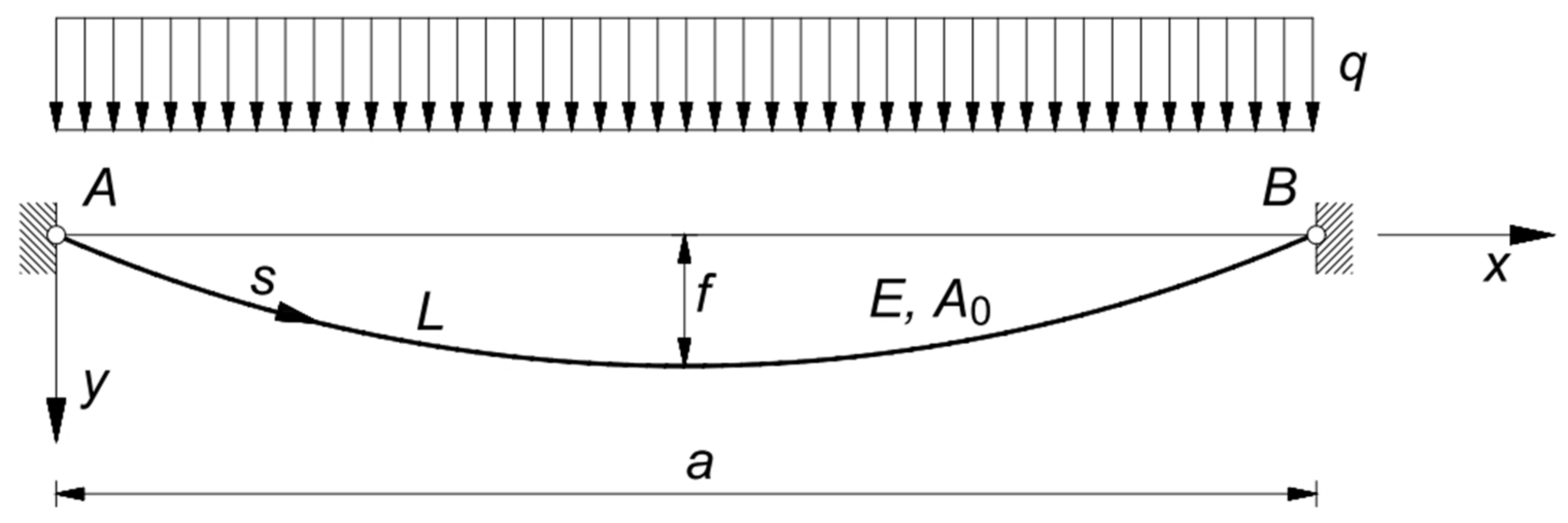
Figure 2.
System of forces acting on the cable portion .

Figure 3.
Virtual deformations of a cable running on a fixed pulley in : .
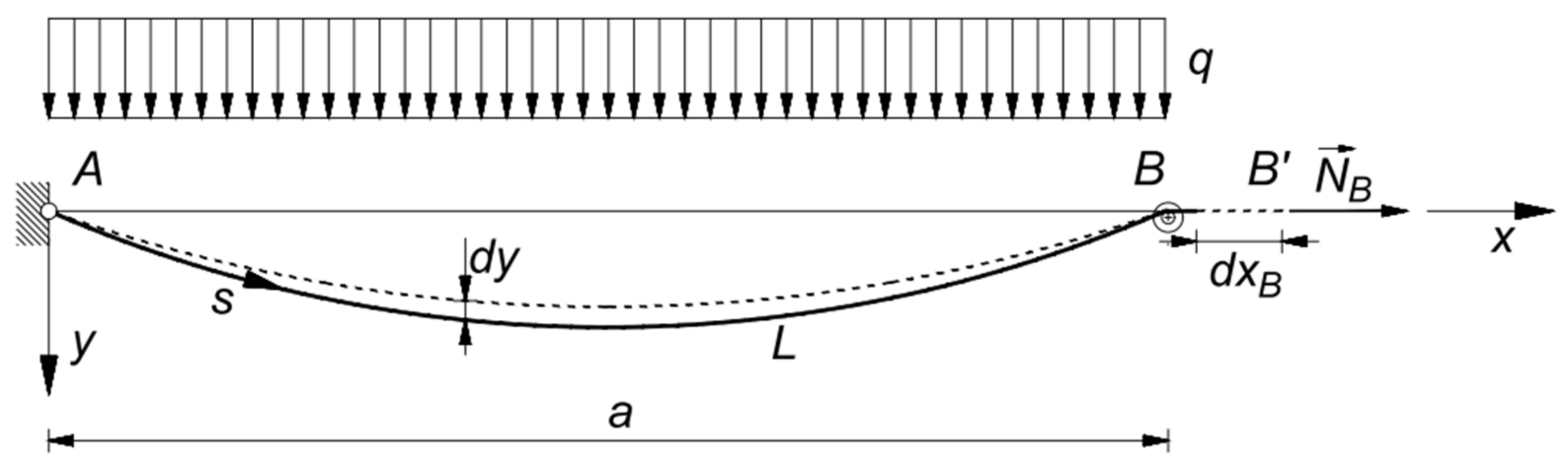
Figure 4.
Virtual deformations of a cable with ends fixed in and .

Figure 5.
diagram for a cable running on a fixed pulley: .

Figure 6.
diagrams parameterized in terms of ( (a) (b) ; (c) ; (d) .

Figure 7.
diagrams parameterized in terms of ((a) (b) .

Figure 8.
diagrams parameterized in terms of (a) (b) .

Figure 9.
diagram for a cable with fixed ends.

Figure 10.
diagrams parameterized in terms of ((a) (b) ; (c) ; (d) .

Figure 11.
diagrams parameterized in terms of ((a) (b) .

Figure 12.
diagrams parameterized in terms of (a) (b) .

Figure 13.
diagrams parameterized in terms of ((a) (b) .

Figure 14.
diagrams parameterized in terms of ((a) (b) .

Figure 15.
diagrams parameterized in terms of ((a) (b) .

Figure 16.
diagrams parameterized in terms of ((a) (b) .

Figure 17.
diagrams parameterized in terms of ((a) (b) .

Figure 18.
diagrams parameterized in terms of ((a) (b) .

Figure 19.
diagrams parameterized in terms of ((a) (b) .

Figure 20.
diagrams parameterized in terms of ((a) (b) .

Figure 21.
Finite element model of the cable: (a) (b) ; (c) (d) .

Figure 22.
diagram for the cable: loading phase ; imposed displacement phase .

Figure 23.
Comparison between theoretical curves parameterized in terms of and nonlinear finite element analysis results ((a) (b) .
Figure 23.
Comparison between theoretical curves parameterized in terms of and nonlinear finite element analysis results ((a) (b) .


Table 1.
Relevant mechanical properties of natural and artificial cable and rope materials.
| Cable Material | Density [kg/m3] | [GPa] | [MPa] | |
|---|---|---|---|---|
| Aramid fiber (high modulus) | 1440 | 112 | 3000 | 2.68% |
| Aramid fiber (normal modulus) | 1440 | 70.5 | 2900 | 4.11% |
| Liquid crystal aromatic polyester (LCP) fiber | 1410 | 66 | 2830 | 4.29% |
| Polybenzoxazole (PBO) fiber | 1560 | 270 | 3950 | 1.46% |
| Carbon fiber 1 | 1560 | 170 | 2500 | 1.47% |
| Carbon fiber 2 1 | 1800 | 240 | 4850 | 2.02% |
| Steel strand | 7850 | 180 | 1770 | 0.98% |
| Steel wire | 7850 | 206 | 1900 | 0.92% |
| Copper | 8940 | 110 | 240 | 0.22% |
| Aluminum | 2700 | 69 | 105 | 0.15% |
| Nylon fiber | 1140 | 4.56 | 610 | 13.38% |
| Polyester fiber | 1380 | 13.8 | 790 | 5.72% |
| Cotton rope | 1540 | 7.9 | 225 | 2.85% |
| Hemp rope | 1490 | 32 | 300 | 0.94% |
| Flax rope | 1540 | 27 | 340 | 1.26% |
| Jute rope | 1500 | 25.8 | 230 | 0.89% |
| Abaca (Manila hemp) rope | 1320 | 30 | 300 | 1.00% |
| Sisal | 1320 | 30 | 250 | 0.83% |
| Silk (silkworm) | 1320 | 10 | 650 | 6.50% |
| Silk (spider) | 1100 | 12 | 900 | 7.50% |
1 Carbon fiber for structural applications [31].
Publisher’s Note: MDPI stays neutral with regard to jurisdictional claims in published maps and institutional affiliations. |
© 2021 by the author. Licensee MDPI, Basel, Switzerland. This article is an open access article distributed under the terms and conditions of the Creative Commons Attribution (CC BY) license (https://creativecommons.org/licenses/by/4.0/).
Share and Cite
MDPI and ACS Style
Croce, P. Tie Rod-Equivalent Non-Linear Constitutive Law for Uniformly Loaded Cables. Materials 2021, 14, 5502. https://doi.org/10.3390/ma14195502
AMA Style
Croce P. Tie Rod-Equivalent Non-Linear Constitutive Law for Uniformly Loaded Cables. Materials. 2021; 14(19):5502. https://doi.org/10.3390/ma14195502
Chicago/Turabian StyleCroce, Pietro. 2021. "Tie Rod-Equivalent Non-Linear Constitutive Law for Uniformly Loaded Cables" Materials 14, no. 19: 5502. https://doi.org/10.3390/ma14195502
Note that from the first issue of 2016, this journal uses article numbers instead of page numbers. See further details here.