Article

Prediction of Axial Capacity of Concrete Filled Steel Tubes Using Gene Expression Programming

by
Kaffayatullah Khan
1,*,
Mudassir Iqbal
2,
Muhammad Raheel
3,
Muhammad Nasir Amin
1,
Anas Abdulalim Alabdullah
1,
Abdullah M. Abu-Arab
1 and
Fazal E. Jalal
4
1
Department of Civil and Environmental Engineering, College of Engineering, King Faisal University, Al-Ahsa 31982, Saudi Arabia
2
Department of Civil Engineering, University of Engineering and Technology Peshawar, Peshawar 25120, Pakistan
3
Department of Civil Engineering, University of Engineering and Technology Mardan, Mardan 23200, Pakistan
4
Department of Civil Engineering, Shanghai Jiao Tong University, Shanghai 200240, China
*
Author to whom correspondence should be addressed.
Materials 2022, 15(19), 6969; https://doi.org/10.3390/ma15196969
Submission received: 10 August 2022 / Revised: 26 August 2022 / Accepted: 1 September 2022 / Published: 7 October 2022

Abstract

:
The safety and economy of an infrastructure project depends on the material and design equations used to simulate the performance of a particular member. A variety of materials can be used in conjunction to achieve a composite action, such as a hollow steel section filled with concrete, which can be successfully utilized in the form of an axially loaded member. This study aims to model the ultimate compressive strength (Pu) of concrete-filled hollow steel sections (CFSS) by formulating a mathematical expression using gene expression programming (GEP). A total of 149 datapoints were obtained from the literature, considering ten input parameters, including the outer diameter of steel tube (D), wall thickness of steel tube, compressive strength of concrete (fc’), elastic modulus of concrete (Ec), yield strength of steel (fv), elastic modulus of steel (Es), length of the column (L), confinement factor (ζ), ratio of D to thickness of column, and the ratio of length to D of column. The performance of the developed models was assessed using coefficient of regression R2, root mean squared error RMSE, mean absolute error MAE and comparison of regression slopes. It was found that the optimal GEP Model T3, having number of chromosomes Nc = 100, head size Hs = 8 and number of genes Ng = 3, outperformed all the other models. For this particular model, R2overall equaled 0.99, RMSE values were 133.4 and 162.2, and MAE = 92.4 and 108.7, for training (TR) and testing (TS) phases, respectively. Similarly, the comparison of regression slopes analysis revealed that the Model T3 exhibited the highest R2 of 0.99 with m = 1, in both the TR and TS stages, respectively. Finally, parametric analysis showed that the Pu of composite steel columns increased linearly with the value of D, t and fy.

1. Introduction

Columns are a desideratum in designing the structural elements of a building. Depending upon the locality, application and resource availability, different materials, for instance, concrete, steel and their combination can be utilized for column construction [1,2,3,4,5]. Reinforced concrete (RC) columns are vastly used around the globe due to a number of reasons, i.e., easy availability of their constituent materials, known behavior under different loading conditions, and development of design codes, such as the ACI 318 [6] design manual and Euro code [7], among others. However, hollow steel sections filled with concrete (HSSFC) represent an improved version in contrast to the other traditional RC columns, both in terms of performance as well as construction costs, alongside possessing the merit of no longitudinal and transverse reinforcement requirements [8]. For example, the hollow steel section (from hereon, referred to as HSS) confines the concrete thus improving its mechanical properties while the buckling resistance of the steel section is enhanced due to the presence of concrete. The composite action of the two materials increases the overall strength, stiffness, ductility, buckling resistance of the element, and provides an improved fire resistance. Since concrete is poured inside the HSS, the need for formwork is eliminated and labor cost is also reduced [9,10,11,12,13].
The cross-sections of the HSS used in concrete-filled hollow steel sections (CFSS) exhibit numerous shapes, i.e., circular, rectangular and square, wherein the most common one is circular because of its high confinement performance [14,15,16]. On a global scale, a number of design codes encompasses the provisions for axial and flexure capacity design of the CFSS [17]. Examples include the Eurocode 4: Design of composite steel and concrete structures (EN1994) [7], AISC-360: Specification for structural steel buildings [18], ACI-318 [6], etc. In addition, the behavior of CFSS has been studied by a number of researchers by considering a number of design parameters such as the slenderness ratio, eccentricity ratio, end-moment ratio, thickness of internal steel tube and compressive strength of concrete, in addition to others [19,20,21], using laboratory experiments and numerical modelling. Although the current codes provide enough guidelines about the axial capacity of CFSS columns, however, uncertainties in the nominal and actual mechanical properties of steel and concrete make the design conservative. In this situation, artificial intelligence (AI) models provide an accurate solution based on mechanical properties of steel and concrete.
Besides the experimental studies for developing knowhow about the influence of various input parameters on the structural performance, soft computing (SC)/machine learning (ML)/(AI)/techniques are gaining popularity nowadays, because of their ability to learn from training data so as to formulate a trained algorithm which can be used for accurate prediction of the output(s) [22,23,24,25]. The accuracy of a typical AI model depends on the number of data points used during the training process and the selection of influential input variables (i.e., high Pearson correlation value). Therefore, several studies have been undertaken recently for evaluating the behavior of CFSS columns under different loading conditions. For example, Albero et al. [26] studied the ultimate resisting load of CFSS under unequal eccentricities at both ends. It was found that the application of unequal load eccentricities enhanced the ultimate resisting load with columns having higher slenderness ratio of 27.78. Similarly, neural networks were successfully used for modelling the strength of columns considering fv, fc’ and the diameter and wall thickness of the HSS and they concluded that the ANN model successfully predicted the columns’ performance (coefficient of regression R2 > 0.98 in the training, test and validation phases) and recommended it to be a reliable tool for assessing the columns’ performance based on the ANN-based Monte Carlo method [27]. Likewise, the axial load capacity of a CFSS having a circular cross-section was modelled using Artificial Neural Networks (ANN) and Gene Expression Programming (GEP). For example, Naderpour et al. [28] deployed GEP, ANN and group methods of data handling to predict the compressive strength of columns confined with fiber reinforced polymers. It was observed that the ANN model had the highest accuracy among its competitors, with R2 > 0.98. Similarly, the error percentage (± 20% error range) of the forecasted output by ANN, GEP and GMDH was recorded as 94.7, 84.2 and 88.4%, respectively. Similarly, Azim et al. [29] utilized the GEP approach to develop a prediction model for the compressive arch action capacity of RC beam-column substructures. Again, GEP was successfully used for studying the behavior of H-section steel columns (R2 > 0.94) under blast loading by Momeni et al. [30]. In addition, an empirical equation was also generated from the GEP model for relating the damage index to the displacement/rotational index. Wang et al. [31] studied the blast resistance and residual strength of CFSS considering the thickness of steel tube and cross-section geometry. It was observed that the CFSS retained up to 60% of its ultimate axial loading capacity even after close-range blast loading and that their axial load capacity retention was enhanced with the thickness of steel tubes. Similarly, Zhang et al. [32] also concluded that concrete filled steel tubular columns showed excellent performance against flexural loads under both static and dynamic loads.
A literature survey reveals successful application of different AI techniques, such as ANN, GEP and ANFIS alongside the combination of meta-heuristic optimization algorithms and ML algorithms for predicting the mechanical performance of concrete as well as soils [24,33,34,35,36,37,38,39]. However, the ANN and ANFIS provide lesser insight about the models pertaining to their practical implications, e.g., to derive an empirical relation between the input parameters and output(s), which can further be used for predicting the output(s) and performing parametric and sensitivity analysis [40,41]. In addition, both these models are termed as ‘black-box models’ in the literature [40,41], due to the complex interaction of neurons present in different hidden layers. As a result, a useful empirical relation between the input and output parameters is difficult to develop and has reliability issues [42]. In contrast, the white-box models, such as GEP, can provide a simple and easy-to-use mathematical expression to forecast the output for a specific range of input parameters. Using that expression sensitivity and parametric analyses could enable validation of the developed GEP model [43]. Shahmansouri et al. [44] developed an empirical equation for predicting the fc’ of geopolymer concrete by considering the specimen’s age, concentration of alkaline activator (i.e., NaOH), natural zeolite, silica fume and blast furnace slag content to be the most influential input parameters. Similarly, Naser et al. [45] developed design equations for the structural response of the CFSS by utilizing the Genetic Algorithm (GA) and GEP technique. They concluded that both GA and GEP models outperformed the current design codes, such as Eurocode 4 [7], AISC 360-16 [18] and New Zealand code (NZS 2327) [46]. Both the models had high predictive capability as a majority of the data points ranged within a 10% bounding error. In an effort to develop an empirical relation between the mix design parameters of lightweight foamed concrete, Sami et al. [47] employed GEP by using 191 data points to develop a model which could simulate the influence of input parameters (i.e., amount of cement, fine aggregate, water to cement ratio and foam volume) on two outputs (i.e., dry density and fc’). They revealed that GEP accurately modelled the dry density and fc’ of foamed concrete, as evident from their higher values of the coefficient of determination (R2) (i.e., 0.79 and 0.94, respectively).
In connection to the use of AI models related to predicting the Pu of CFSS columns, Sarir et al. [48] used a dataset of 303 points to compare the performance of a GEP model with ANN model optimized by particle swarm optimization (PSO) algorithm, as listed in Table 1. The concrete compressive strength (fc’), the column length (L), outer diameter (D), tensile yield stress of the steel column (fy), and steel cover thickness (t) were considered as input variables. The best performance was obtained for the GEP model interpreting R2 equaling 0.939. Javed et al. [49] included eccentricities at end supports (et, eb) alongside the previously mentioned variables by employing 227 sample specimens. Khan et al. used an extensive database yielding R2 of 0.9812 for test data; however, the value of MAE recorded was comparatively high. Several other researchers (Ngo et al. [50], Jiang et al. [51], Jayalekshmi et al. [52], Ahmadi et al. [53]) also developed Support Vector Regression (SVR) optimized by Grey Wolf Optimization (GWO), GEP, and ANN models, and evaluated the accuracy in terms of R2. The capabilities of the GEP model were not fully explored by changing its genetic parameters, i.e., number of chromosomes (Nc), genes (Ng) and head sizes (hs) to obtain the best hyperparameters. Nevertheless, this study utilized 10 variables including the confinement factor (ζ) which was not used in the reported literature.
The ANN and various other such hybrid algorithms (e.g., ANFIS) are unable to provide an empirical equation between the inputs and output(s). As a result, GEP is deployed to robustly simulate the ultimate compressive strength (Pu) of the CFSS considering different inputs parameters, i.e., (i) outer diameter of steel tube (D), (ii) wall thickness of steel tube (t), (iii) compressive strength of concrete (fc’), (iv) elastic modulus of concrete (Ec), (v) yield strength of steel (fv), (vi) elastic modulus of steel (Es), (vii) length of the column (L), (viii) confinement factor (ζ), (ix) D/t ratio of column and (x) the L/D ratio of column. The performance of the developed model was assessed using different statistical indices, i.e., R2, root mean square error (RMSE), mean absolute error (MAE), comparison of regression slopes, predicted to experimental (P/E) ratios. In addition, parametric and sensitivity analyses were also carried out to assess the effect and contribution of input parameters on the Pu of CFSS.
The flow of the paper is that the database is compiled, and the GEP modelling is performed. The formulated GEP model is obtained after undertaking several trials and the effect of genetic parameters on the model performance is studied. After selecting the most optimal trial, the mathematical expression is determined. A variety of performance measures (error indices) were calculated to check the performance of the optimal model. Parametric and sensitivity analyses were also performed for the input parameters considered in the formulated GEP model.

2. Methodology

2.1. Database Compilation

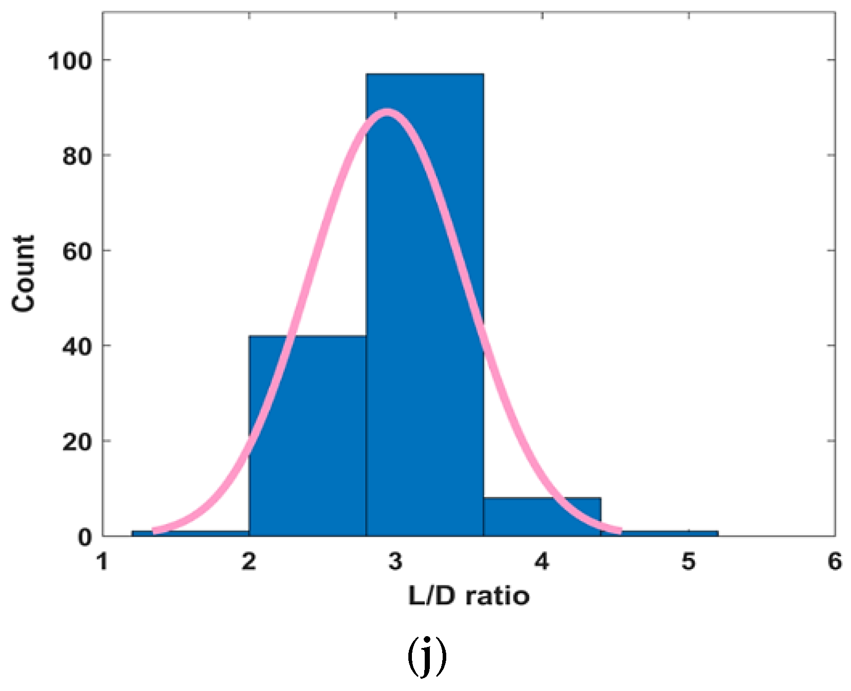
The database was compiled from the work published by Bardhan et al. [55], which comprises a total of 149 datapoints of which 104 datapoints were used for the training (TR) phase whereas the remaining 49 points were utilized for the testing (TS) phase. Ten input parameters, i.e., D, t, fc’, Ec, fy, Es, L, ζ, ratio of D and t (i.e., D/t) and the ratio of L and D (i.e., L/D) were considered in order to model their influence on the Pu of CFSS using a genetic programming approach. The descriptive statistics of the dataset used for developing the GEP model are listed in Table 2. In order to indicate the frequency distribution of input parameters, the departure of data from the horizontal symmetry (skewness) and the sharpness of the central peak, relative to a standard normal distribution curve [56], the frequency histograms of the input parameters along with their respective normal distribution fit are shown in Figure 1. The values of kurtosis and skewness in Table 2, are in accordance with the aforementioned normal distribution curves. For example, the values of kurtosis and skewness are positive for all the input parameters except for Ec and Es, respectively. Referring to Figure 1a–c,e–j), the distribution is peaked with a thick tail while Figure 1d shows that the distribution of Ec is flatter, which justifies the negative kurtosis value. Similarly, the negative value of skewness for Es can be corroborated from Figure 1a, since the distribution has a fatter tail on its left side.

2.2. GEP Modelling

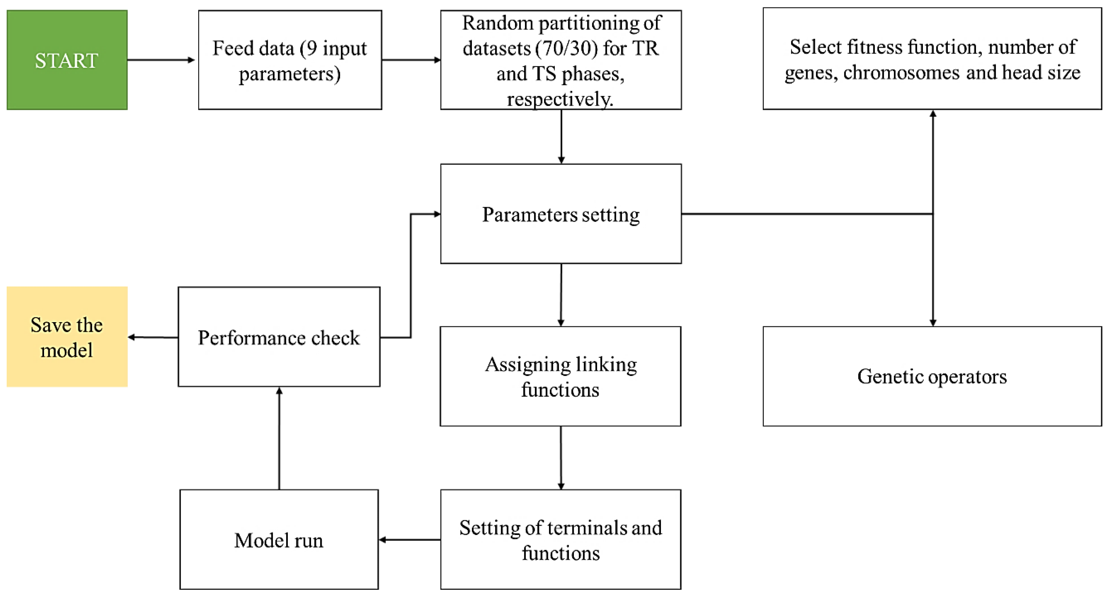
GeneXprotools v5.0, developed by Candida Ferreira (Portugal), was employed for developing the desired GEP models. For this purpose, the data was fed into the GEP interface. Afterwards, the dataset was divided into two subsets namely; the TR dataset (70%) and the TS dataset (30%). As a result, 104 datapoints were used for the TR phase whereas the remaining 45 datapoints were used during the TS phase. The option of normalization is readily available in the data tab of this tool; however, the authors did not utilize this option in the current study and the models were trained using the actual values. The authors opine that the statistical models are based upon the descriptive statistics of the given dataset. Similar studies have been widely reported in the past literature [57,58]. In order to achieve the best optimal model, the hyperparameter settings of GEP parameters were adjusted accordingly. For example; the number of chromosomes (Nc) were varied from 30 to 200, the number of genes (Ng) from 3 to 5 and, the head size (Hs) from 8 to 12. Similarly, it was observed that the addition function provides the optimal performance. This was achieved by exploring different linking functions (+, −, ×, /). The details of the genetic parameters settings, i.e., mutation, transposition, and recombination rates are given in Table 3. The details of 11 number of trials employing different values of hyperparameters and the resulting model performance in terms of R2, RMSE and MAE for both the TR and TS phases, respectively, are shown in Table 4. Moreover, Figure 2 shows the flowchart of GEP modelling. The process starts with feeding the input parameters data followed by the random partitioning of datasets. The process is continued by selecting the fitness function, Nc, Hs, Ng and assigning suitable genetic operators. After assignment of linking functions and terminals setting, the model is run and its performance can be checked using different statistical tools such as R2, RMSE and MAE, as shown in Equations (1)–(3), respectively.
R 2 = ( i = 1 n ( e i e ¯ i ) ( p i p ¯ i ) i = 1 n ( e i e ¯ i ) 2 i = 1 n ( p i p ¯ i ) 2 ) 2
R R M S E = 1 | e ¯ | i = 1 n ( e i p i ) 2 n
M A E = i = 1 n | e i p i | n
where ei and pi are the ith experimental and predicted output values, respectively; e ¯ i and p ¯ i are the average values of the experimental and predicted output values, respectively, and n are the total samples.
A trial and error approach was used for setting the GEP parameters, such that an optimal performing model with the best hyperparameter settings could be obtained. This practice would help avoiding overfitting the data during the TR phase, and, subsequently, improve their performance in the TS phase. In the past, researchers have addressed the problem of overfitting [59]. For example, Gandomi and Roke [60] selected the model with minimum objective function (OF) value which varies from 0 to maximum value, with the model having OF ≈ 0 is considered to have the best performance. Here, statistical evaluation was used to select a non-overfitted model. Table 5 shows the ideal values of the three performance indices, i.e., R2, RMSE and MAE, used to assess the models’ performance.

3. Results & Discussion

3.1. Variation of Genetic Parameters

Table 4 depicts that a total of 11 trials (Model T1 to T11) were conducted by varying the different parameters of the GEP model (Nc, Hs and Ng). As discussed earlier, the hyperparameters of GEP models were varied to achieve an optimal GEP model. A total of 11 trials (i.e., Model T1 to T11) were employed with varying values of Nc, Ng and Hs (Table 4). Firstly, the values of Nc were varied from 30 to 200, while keeping the Hs and Ng constant (i.e., 8 and 3, respectively). In the second stage, the Hs was changed from 8 to 12, while keeping both Nc and Ng constant. Similar practice was followed for Ng as well. The values of Nc, Hs and Ng for the best performing model (Model T3) came out to be 100, 8 and 3, respectively. For all the trials, the performance of the models was assessed using R2, RMSE and MAE. It is evident from Table 4 that the model T3 has the highest R2 and, lowest RMSE and MAE, in both the TR and TS phases, respectively.
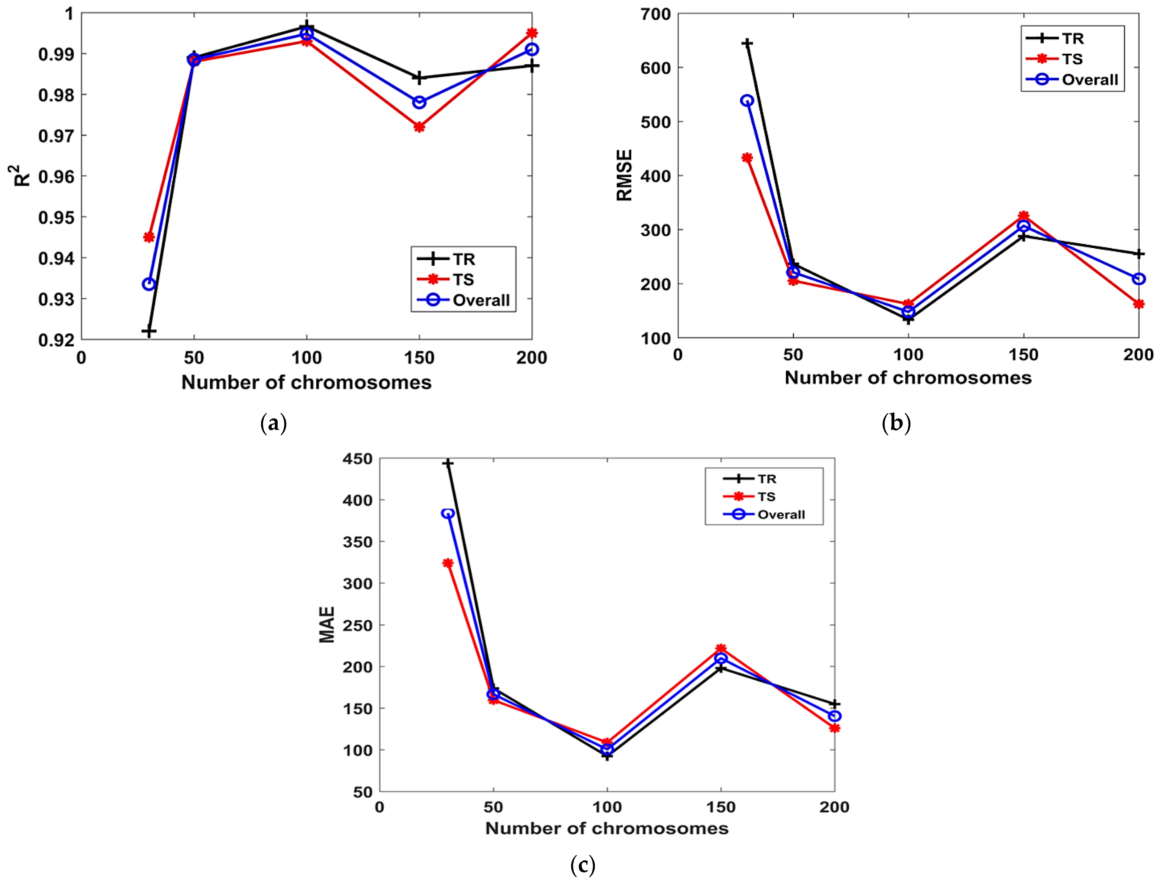
Figure 3 shows the influence of Nc on the R2, RMSE and MAE of the models, in both the TR and TS phases, respectively. It can be seen from Figure 3a that, the value of R2 increases with the Nc till it drops for Nc = 150. A further increase in Nc (i.e., from 150 to 200) enhances the R2 again. Similar improvement in the performance of the models with the increase in Nc up to 100 can be observed in Figure 3b,c. It is evident from these Figures that the value of RMSE and MAE plummets with the increase in Nc; however, the model performs poorly for Nc = 150 as evident from its lower R2 = 0.98, 0.97, higher RMSE = 287.8, 325.5, and MAE = 198.1, 221.7, in the TR and TS phases, respectively.
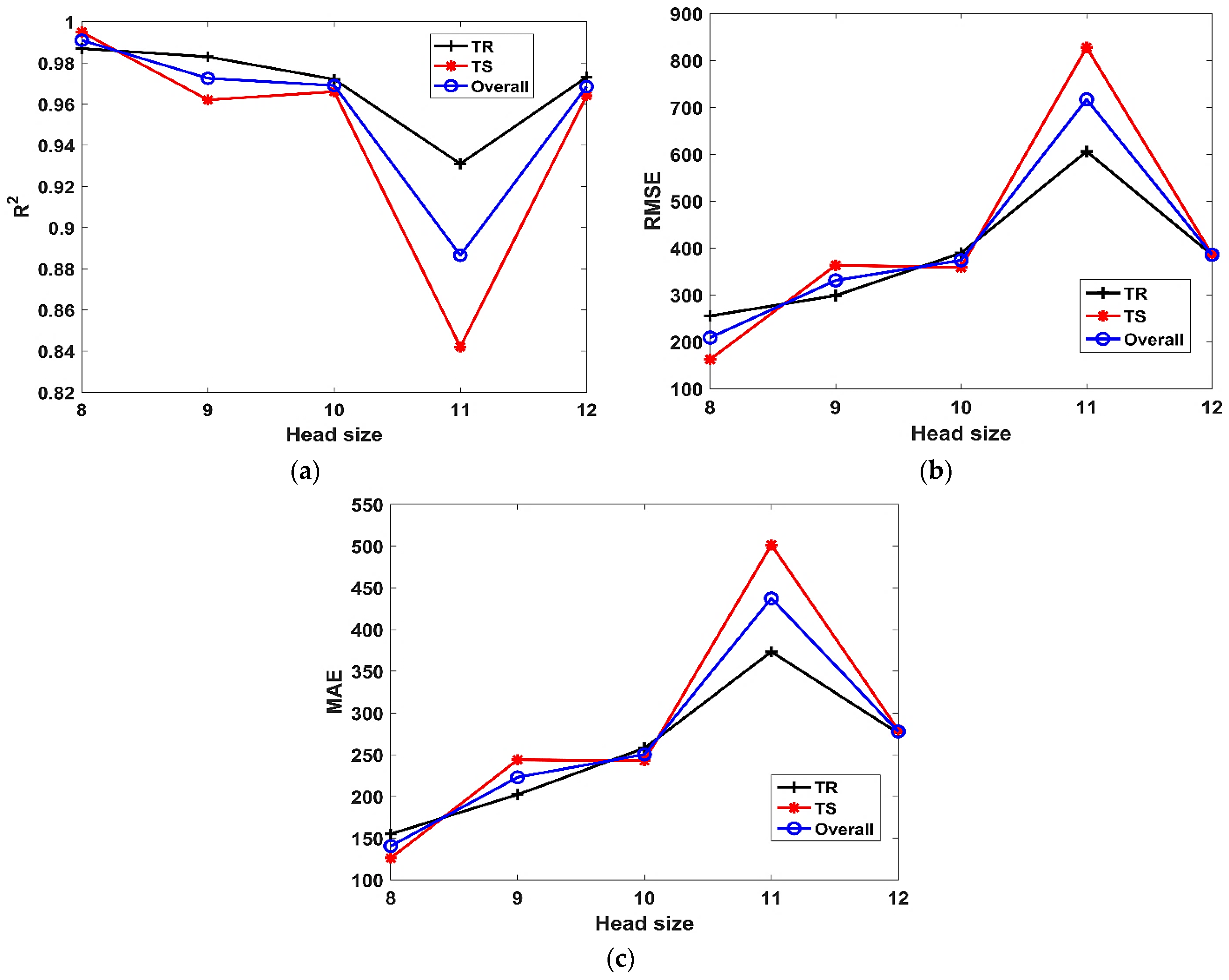
The influence of Hs on the performance of models (both TR and TS phases) in terms of R2, RMSE and MAE can be observed in Figure 4a–c, respectively. It is evident from Figure 4a that, R2 decreases with increasing Hs. The model depicts immensely poor performance for Hs = 11; however, upon further increase in the Hs = 12, the value of R2 improves. A similar trend can be observed in the case of Figure 4b,c, wherein the RMSE and MAE increase with the Hs. The model performs poorly as is evident from its high RMSE and MAE values for Hs = 11. The influence of Ng on the performance of models (TR and TS phases) in terms of R2, RMSE and MAE can be observed in Figure 5a–c, respectively. Considering the TR phase, it is evident from Figure 5a, that the value of R2 increases with the increase in the Ng up to 4. Further increase in value of Ng (i.e., 4 to 5) lowers the value of R2. Similar trend can be observed from Figure 5b,c, wherein the value of RMSE and MAE decrease with the value of Ng (i.e., 3 to 4). When the Ng is further increased from 4 to 5, the accuracy of the model decreased as is evident from its high RMSE and MAE values for Ng = 5. However, the performance of the model improves at higher Ng in the TS phase, as evident from its higher R2 value = 0.98, and lower RMSE and MAE values of 288.9 and 218.5, respectively.

3.2. Models’ Performance

3.2.1. Statistical Evaluation

It can be seen from Table 4 that the performance of the Model T3 is better (R2 = 0.99 for both the TR and TS phase) followed by Model T5 (R2 = 0.98 in TR phase, and 0.99 for TS phase). The observed values of R2 shows a good agreement between the predicted and experimental values. However, a model cannot be declared as the “best performing model” solely on the basis of R2. Other statistical error indices must also be considered, such as RMSE and MAE, in addition to others. In this regard, the values of RMSE and MAE were also studied in the current study while assessing the performance of different models. It is evident from Table 4 that, in addition to a higher R2 value, Model T3 exhibited the lowest RMSE (133.4 in TR phase, and 162.2 in TS phase) and MAE (92.4 in TR phase and 108.7 in TS phase). Similarly, the Model T5 performed as second-best model having RMSE = 255.1 in the TR phase, and, RMSE = 478.2, and MAE = 386.6 in the TS phase, respectively. Model T2 also performed better as it possessed the second highest R2 and second lowest value of RMSE in the TR phase, respectively. The ranking of the models based on the different statistical indices has also been shown in Table 6.

3.2.2. Comparison of Regression Slopes

Prediction models can be evaluated by plotting a trend line between the experimental and predicted values. This assessment method has also been used in this study and as a result, regression slopes have been plotted for all the 11 models, in both the TR and TS phases, respectively. It is noteworthy to mention that an ideal trend line has a slope “m” value of unity (=1.0) and, its angle of inclination with both the X- and Y-axis in the cartesian coordinate system equals 45°. The performance of the model is considered to be reliable and accurate provided the plot between the forecasted and experimental values follow the ideal trend line (i.e., inclined at an angle of 45° with the X-axis). A regression line whose m value approaches one, and, its correlation value i.e., R 0.8 are considered reliable in forecasting new data [61].
Figure 6 shows the values of R2 and m for both the TR and TS phases, respectively. It is evident from the Figure 6 that R2 exceeds 0.90 for all of the models. In the TR phase, Model T3 has the best fit with an R2 value of 0.99 and m = 1 whereas, Model T1 has a lower value of R2 = 0.92 and m = 0.91. Similarly, the performance of the models improved in the TS phase, as indicated from the higher R2 values and the m values becoming closer to one. All the models have R2 ≥ 0.90. It can also be observed from Figure 6 that, the highest value of m = 1 has been obtained for the optimal model T3 in both the TR and TS phases, respectively. However, Figure 7 shows that in addition to model T3, other models (except T2 and T6) had m values equaling one. It is important to mention here that for m = 1, the slope of the regression line will be exactly 45°. In comparison to other models, the values of ‘m’ and R2 observed for the Model T3 are closer to one. Therefore, it can be concluded that the Model T3 is the best performing model, compared to the others.

3.2.3. Model Predicted to Experimental Ratio (P/E)

The performance of the generated models as a result of different trials (by varying Nc, Hs and Ng) was further studied using the P/E ratio. Figure 7a,b depict the distribution of the P/E ratios for the optimal performing Model T3 in the TR and TS phases, respectively. The bin range has been varied between 0 and 2 using a uniform interval of 0.2. It can be observed from both Figure 7a,b that most of the P/E values (higher frequencies) concentrated in the bin range proximal to one. This serves another statistical check in evaluating the performance of the formulated model and acts as visual justification in case of the optimal performance Model T3.

3.3. GEP Formulations

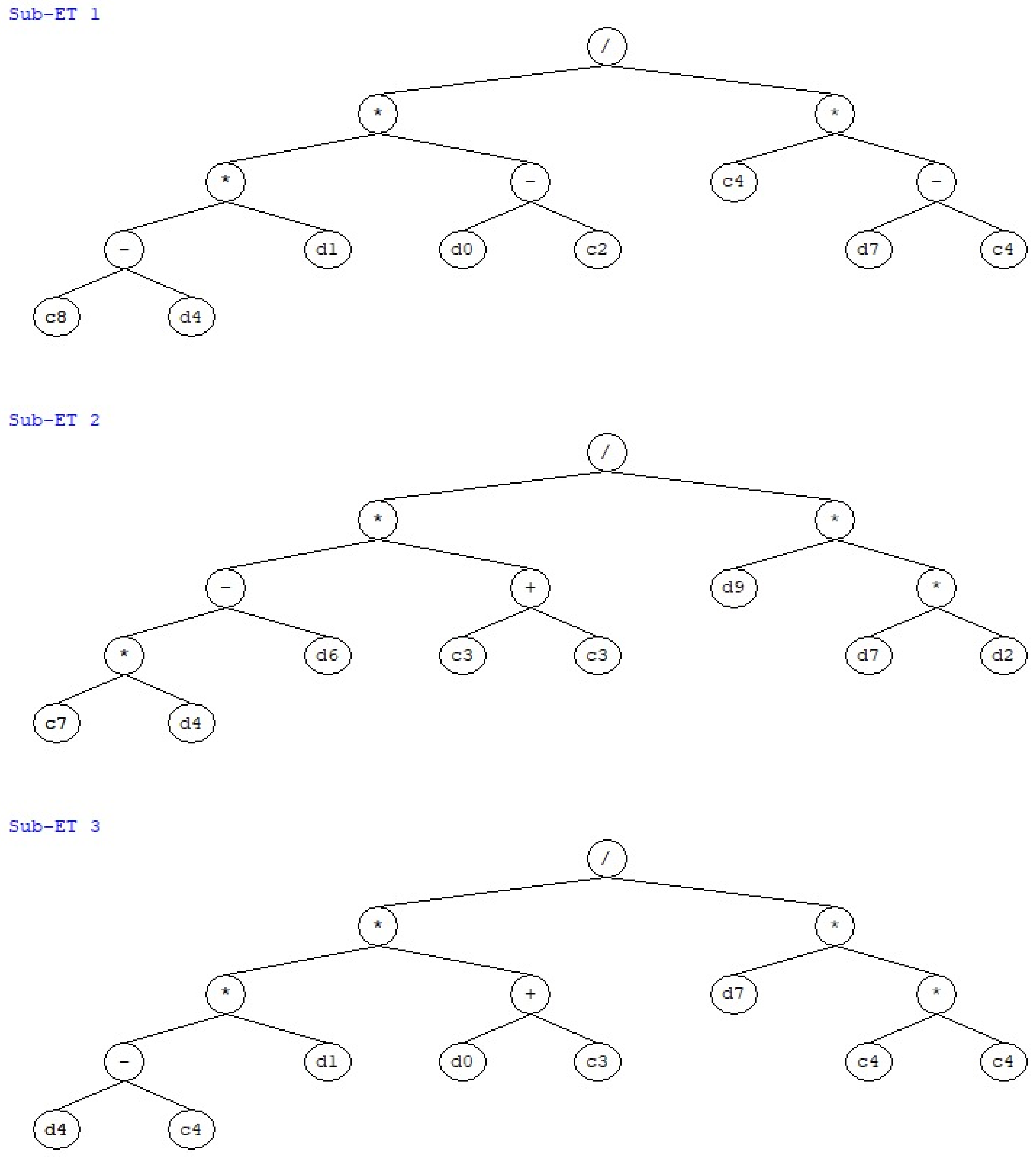
In addition to successful simulation of the Pu of CFSS considering a number of input parameters, another novel achievement of this research work is to obtain an empirical equation which can be used for predicting the Pu of the CFSS using the different input variables. For this purpose, the optimal performing Model T3 was used to develop the empirical equation. The expression tree for the Model T3 (Figure 8) and the MATLAB model were utilized to obtain the mathematical expression, which can be further used for forecasting the Pu of the CFSS, and, sensitivity and parametric analysis can be performed as well. As a result, Equation (4) was obtained, which is able to predict the Pu of CFSS using various input variables (i.e., D, t, fc’, Ec, fv, Es, L, ζ, ratio of D to thickness of column and, the ratio of length to D of column). It is highly recommended to use the prediction equation for input variables whose range and other details have already been discussed in Section 2.1 [62,63].
P u = ( 36.9 f y ) ( D 25.2 ) t 17.2 ( ζ 17.2 ) + ( ( 2.3 f y ) L ) 21.2 L / D ζ f c + ( ( f y 17.2 ) t ) ( D + 2.2 ) ζ 34.4
The values of the constants (c), as present in Figure 8 are as follows:
Sub-ET1: c8 = −36.9; c2 = 25.2; c4 = 17.2; Sub-ET2: c7 = 2.3; c3 = 10.6; Sub-ET3: c4 = 17.2; c3 = 2.2;
Whereas, d0, d1, d2, d3, d4, d5, d6, d7, d8, d9 represents the input parameters such as D, t, fc’, Ec, fy, Es, L, ζ, D/t and L/D, respectively.
This Equation (4) is a simple-to-use mathematical expression for designers and practitioners, who can robustly determine the Pu of the CFSS when the easily determinable parameters are available.

3.4. Parametric and Sensitivity Analysis

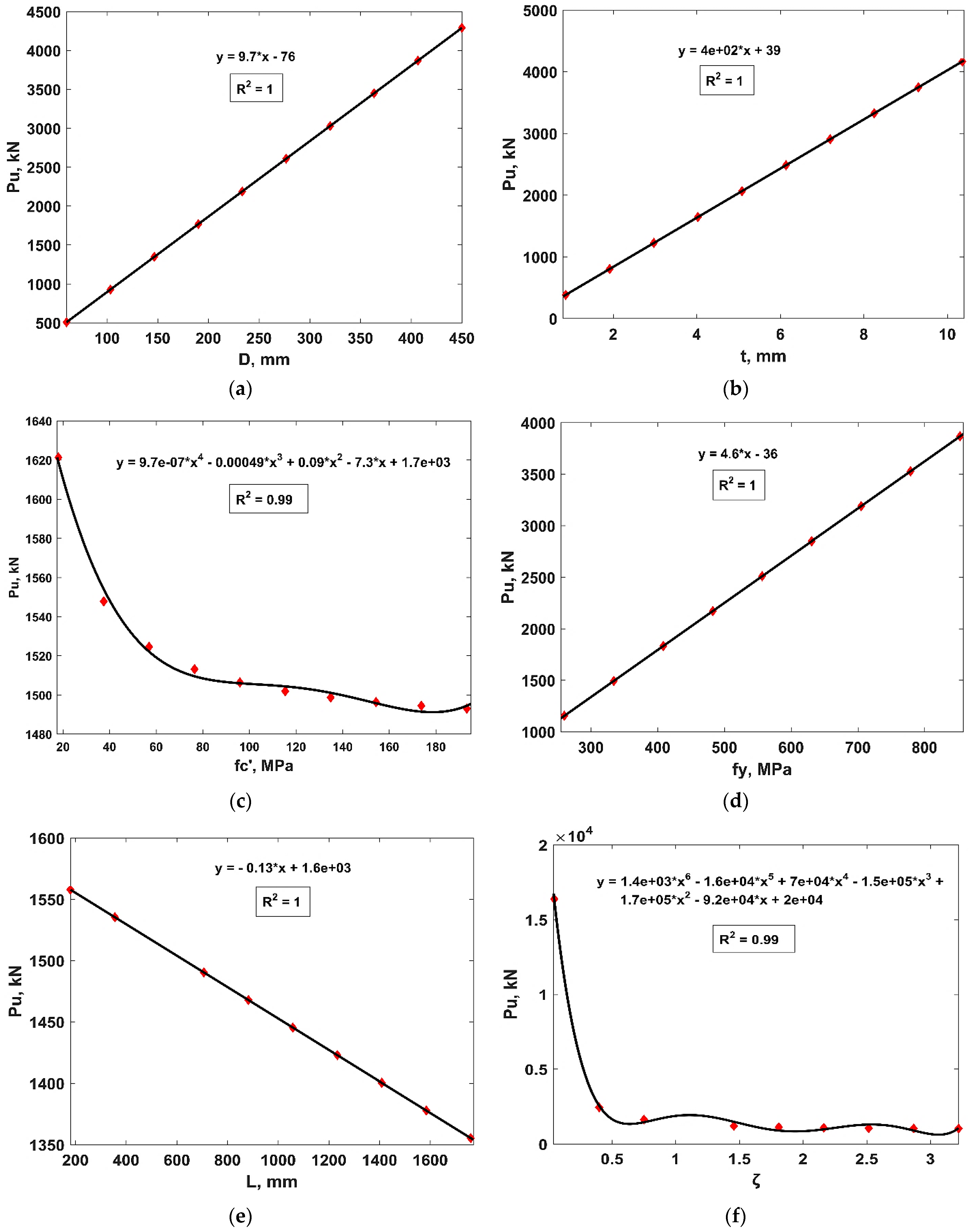
The reliability of different AI models can be verified by conducting parametric analysis of the input features. In this study, the parametric analysis was also carried out for all the input parameters viz., D, t, fc’, Ec, fv, Es, L, ζ, ratio of D to column, and the ratio of L to D, in order to evaluate their effect on the resulting Pu of the CFSS columns. Table 7 shows the possible combination of the study input parameters, considered for the parametric analysis. Hence, a dataset was generated such that one of the input variables (first variable, D) was varied between its extreme values (lower to maximum value in the dataset) in equal increments, while, keeping the remaining input parameters at their average values. In the next step, a second input parameter (i.e., t) was altered in a similar manner, while, keeping the other input features at their mean values. This practice was repeated for all the input parameters. The prediction equation (as given by Equation (1)) was utilized to obtain the corresponding change in the target variable. The range of input variables and their corresponding influence on the Pu of CFSS columns was plotted to study their relationship. The net change in the output (Pu of CFSS columns) due to changing a particular input feature, was calculated in terms of weighted percentage, in order to find the sensitivity of each input attribute, as well. Note that the sensitivity analysis shows the response of the prediction model by varying the input parameters [64]. The relative contribution of the input parameters can be studied using this analysis as shown in Equation (5) and (6) below.
P i = f max ( s i ) f min ( s i ) × N
S e n s i t i v i t y ( % ) = P i i = 1 n P j × 100
Here, f m a x ( s i ) and f m i n ( s i ) refer to the maximum and minimum GEP estimated values for the i’th input domains, where the remaining input factors = 1. The value of sensitivity analysis is between 0 and 1 which depicts the relative contribution of input parameters among each input attribute as well as the predicted output variable.
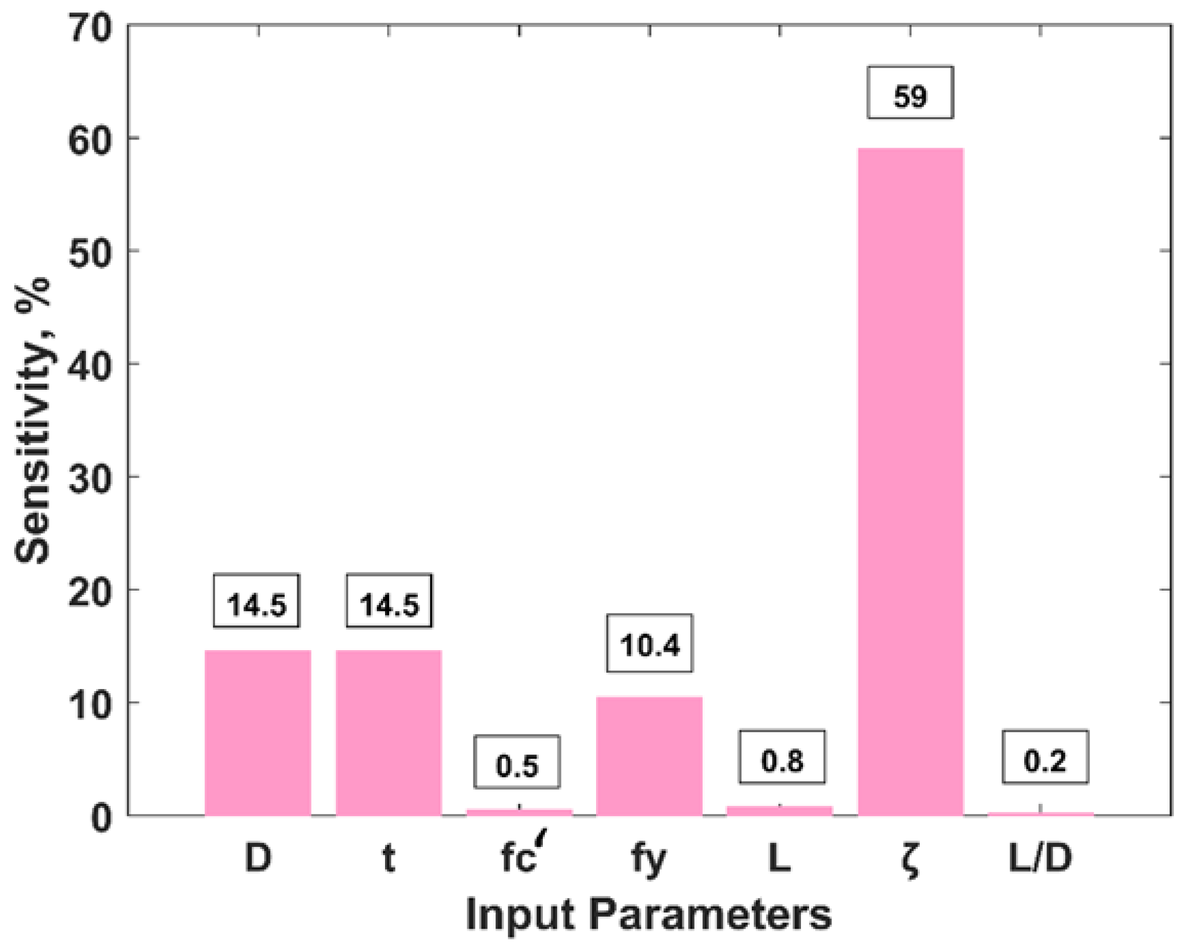
Figure 9 shows the variation of the Pu of CFSS columns in response to the change in each input variable, as explained above. It is apparent from Figure 9a,b,d that the Pu of CFSS columns increases linearly with the values of D, t and fy while it decreases with the amount of fc’, L, ζ and L/D ratio, as is evident from Figure 9c,e–g), respectively. The parametric analysis also revealed that the input parameters, such as Ec, Es and the ratio of D/t had least influence on the output parameter, i.e., Pu. Moreover, Figure 9c,f reveal that the value of Pu plummets with the increasing values of fc’ and ζ. Similarly, different equations such as linear, 3-, 4- and 6-degree polynomial equations were fitted to the resulting parametric analysis, which illustrate good agreement with the datapoints, i.e., all the parameters exhibit R2 ≥ 0.99. The sensitivity analysis of the input variables (as shown in Figure 10) reveals that ζ has the highest value of sensitivity (59%) followed by D and t (14.5%, each). It is also evident that L/D has the least sensitivity value = 0.2. This can be explained from the fact that the confinement of concrete enhances its strength and ductility, which enhances the Pu. Similarly, increasing value of D and t reduces the slenderness ratio of a column and enables the steel casing to withstand higher tensile stresses imparted by the confined concrete, respectively [21].

4. Conclusions

This research study aims to model the ultimate compressive strength (Pu) of concrete-filled hollow steel sections (CFSS) columns by formulating an empirical relation between the output and input parameters. A total of 149 datapoints were taken from the literature, considering a number of input parameters such as outer diameter of steel tube (D), wall thickness of steel tube, compressive strength of concrete, elastic modulus of concrete (Ec), yield strength of steel (fv), elastic modulus of steel (Es), length of the column (L), confinement factor (ζ), ratio of D to thickness of column and the ratio of length to D of column. Different trials were undertaken to develop GEP models using various settings of the hyperparameters.
  • The performance of the developed models was assessed using variety of performance indices, i.e., R2, RMSE, MAE and comparison of regression slopes. It was found that Model T3 having Nc = 100, Hs = 8 and Ng = 3 was the optimally performing model among all others. The model exhibits the highest R2 value of 0.99, and the lowest RMSE = 133.4 and 162.2 and MAE = 92.4 and 108.7, in the training and testing phases, respectively.
  • Similarly, the comparison of regression slopes analysis reveals that the Model T3 possess the highest value of R2 equaling 0.99 and m = 1, which represents its high performance and robustness.
  • Finally, the parametric analysis depicts that the Pu of CFSS columns increases linearly with the value of D, t and fy while, Ec, Es and the ratio of D/t had the least influence on the output parameter. The sensitivity analysis of input variables reveals that the ζ is recorded to have the highest value of sensitivity (59%) whereas L/D has the least effect (i.e., 0.2%) in governing the Pu of the CFSS.
  • It is highly recommended to use the prediction equation (Equation (4)) for input variables whose range and other details are considered in the descriptive statistics of the current study. The following simple-to-use mathematical expression can be used to predict the Pu of the CFSS with higher accuracy.

Author Contributions

Conceptualization, K.K.; Data curation, M.I. and F.E.J.; Formal analysis, F.E.J.; Funding acquisition, K.K.; Investigation, M.I., M.R., A.A.A., A.M.A.-A. and F.E.J.; Methodology, M.R., M.N.A., A.A.A., A.M.A.-A. and F.E.J.; Project administration, K.K.; Resources, K.K.; Software, M.I. and F.E.J.; Validation, M.N.A.; Visualization, M.N.A.; Writing – original draft, K.K., M.I., M.R. and F.E.J. All authors have read and agreed to the published version of the manuscript.

Funding

This work was supported by the Deanship of Scientific Research, Vice Presidency for Graduate Studies and Scientific Research, King Faisal University, Saudi Arabia [Project No. GRANT762]. The APC was funded by the same “Project No. GRANT762”.

Institutional Review Board Statement

Not applicable.

Informed Consent Statement

Not applicable.

Data Availability Statement

The data used in this research have been properly cited and reported in the main text.

Acknowledgments

The authors acknowledge the Deanship of Scientific Research, Vice Presidency for Graduate Studies and Scientific Research, King Faisal University, Saudi Arabia [Project No. GRANT762]. The authors extend their appreciation for the financial support that has made this study possible.

Conflicts of Interest

The authors declare no conflict of interest.

References

  1. Sun, Z.; Chen, Y.; Xu, S.Y.; Sun, Y.; Wu, G. Shaking table test of concrete columns hybrid reinforced by steel/FRP bars. J. Build. Eng. 2022, 48, 103938. [Google Scholar] [CrossRef]
  2. Melo, J.; Afshan, S.; Rossetto, T.; Varum, H.; Arêde, A. Experimental and numerical investigation of the cyclic response of stainless steel reinforced concrete columns. Eng. Struct. 2022, 252, 113607. [Google Scholar] [CrossRef]
  3. Zhao, X.; Wen, F.; Yan, S. Behavior of multi-steel reinforced concrete columns with encased steel H-sections. Eng. Struct. 2022, 264, 114463. [Google Scholar] [CrossRef]
  4. Zhuang, M.-L.; Sun, C.; Dong, B. Experimental and numerical investigations on seismic performance of HTRB630 high-strength steel bars reinforced concrete columns. Case Stud. Constr. Mater. 2022, 17, e01185. [Google Scholar] [CrossRef]
  5. Golewski, G.L. A novel specific requirements for materials used in reinforced concrete composites subjected to dynamic loads. Compos. Struct. 2019, 223, 110939. [Google Scholar] [CrossRef]
  6. ACI 318-14; ACI Committee 318, Building Code Requirements for Structural Concrete (ACI 318-14): Commentary on Building Code Requirements for Structural Concrete (ACI 318R-14)—An ACI Standard and Report. American Concrete Institute: Farmington Hills, MI, USA, 2014.
  7. EN1994-1; Design of Composite Steel and Concrete Structures—Part 1-1: General Rules and Rules for Buildings. European Committee for Standardization: Brussels, Belgium, 1994.
  8. Radovanovic, M.M.L.; Nikolic, J.Z.; Radovanovic, J.R.; Kostic, S.M. Structural Behaviour of Axially Loaded Concrete-Filled Steel Tube Columns during the Top-Down Construction Method. Appl. Sci. 2022, 12, 3771. [Google Scholar] [CrossRef]
  9. Zhang, J.; Liu, Y.; Chen, Z.; Cai, R.; Li, X. Seismic behavior of high-strength concrete-filled square steel tube columns reinforced with ultrahigh-strength reinforcing bars. Structures 2021, 34, 3125–3140. [Google Scholar] [CrossRef]
  10. Shao, Z.; Zha, X.; Wan, C. Design method of fire-resistance capacity of reinforced-concrete-filled steel tube column under axial compression. Fire Saf. J. 2022, 129, 103572. [Google Scholar] [CrossRef]
  11. Zhang, T.; Ding, F.X.; Liu, X.M.; Yu, Z.W. Seismic behavior of terminal stirrup-confined concrete-filled elliptical steel tube columns: Experimental investigation. Thin-Walled Struct. 2021, 167, 108251. [Google Scholar] [CrossRef]
  12. Huang, Y.; Zhao, P.; Lu, Y.; Zhang, H. Push-out tests of CFST columns strengthened with self-compacting and self-stressing concrete filled square steel tube. J. Constr. Steel Res. 2022, 193, 107263. [Google Scholar] [CrossRef]
  13. Feng, W.; Wang, Y.; Sun, J.; Tang, Y.; Wu, D.; Jiang, Z.; Wang, J.; Wang, X. Prediction of thermo-mechanical properties of rubber-modified recycled aggregate concrete. Constr. Build. Mater. 2022, 318, 125970. [Google Scholar] [CrossRef]
  14. Zhao, P.; Huang, Y.; Liu, Z.; Wang, H.; Lu, Y. Experimental research on seismic performance of steel fiber-reinforced recycled concrete-filled circular steel tube columns. J. Build. Eng. 2022, 54, 104683. [Google Scholar] [CrossRef]
  15. Wang, X.; Fan, F.; Lai, J. Strength behavior of circular concrete-filled steel tube stub columns under axial compression: A review. Constr. Build. Mater. 2022, 322, 126144. [Google Scholar] [CrossRef]
  16. Jahangir, H.; Soleymani, A.; Esfahani, M.R. Investigating the Confining Effect of Steel Reinforced Polymer and Grout Composites on Compressive Behavior of Square Concrete Columns. Iran. J. Sci. Technol. Trans. Civ. Eng. 2022, 1–17. [Google Scholar] [CrossRef]
  17. Tang, Y.; Zhu, M.; Chen, Z.; Wu, C.; Chen, B.; Li, C.; Li, L. Seismic performance evaluation of recycled aggregate concrete-filled steel tubular columns with field strain detected via a novel mark-free vision method. Structures 2022, 37, 426–441. [Google Scholar] [CrossRef]
  18. ANSI/AISC 360-16; Specification for Structural Steel Buildings. American Institute of Steel Construction (AISC): Chicago, IL, USA, 2016.
  19. Won, D.; Kim, S.; Seo, J.; Kang, Y.-J. Experimental Study of Composite Hollow RC Column under Uniaxial Compressive Load. Appl. Sci. 2019, 9, 373. [Google Scholar] [CrossRef] [Green Version]
  20. Lin, S.; Li, Z.; Lu, Z.-H.; Zhao, Y.-G. Experimental study on the behavior of circular ultra-high strength concrete-filled steel tube columns subjected to unequal end moments. Eng. Struct. 2022, 267, 114709. [Google Scholar] [CrossRef]
  21. Ci, J.; Ahmed, M.; Liang, Q.Q.; Chen, S.; Chen, W.; Sennah, K.; Hamoda, A. Experimental and numerical investigations into the behavior of circular concrete-filled double steel tubular slender columns. Eng. Struct. 2022, 267, 114644. [Google Scholar] [CrossRef]
  22. Mangalathu, S.; Jeon, J.S. Classification of failure mode and prediction of shear strength for reinforced concrete beam-column joints using machine learning techniques. Eng. Struct. 2018, 160, 85–94. [Google Scholar] [CrossRef]
  23. Munir, M.J.; Kazmi, S.M.S.; Wu, Y.F.; Lin, X.; Ahmad, M.R. Development of novel design strength model for sustainable concrete columns: A new machine learning-based approach. J. Clean. Prod. 2022, 357, 131988. [Google Scholar] [CrossRef]
  24. Santarsiero, G.; Mishra, M.; Singh, M.K.; Masi, A. Structural health monitoring of exterior beam–column subassemblies through detailed numerical modelling and using various machine learning techniques. Mach. Learn. Appl. 2021, 6, 100190. [Google Scholar] [CrossRef]
  25. Naderpour, H.; Mirrashid, M.; Parsa, P. Failure mode prediction of reinforced concrete columns using machine learning methods. Eng. Struct. 2021, 248, 113263. [Google Scholar] [CrossRef]
  26. Albero, V.; Ibañez, C.; Hernández-Figueirido, D.; Piquer, A. Experimental analysis on circular concrete-filled steel tubular beam-columns under unequal load eccentricities. Eng. Struct. 2022, 259, 114206. [Google Scholar] [CrossRef]
  27. Irandegani, M.A.; Zhang, D.; Shadabfar, M. Probabilistic assessment of axial load-carrying capacity of FRCM-strengthened concrete columns using artificial neural network and Monte Carlo simulation. Case Stud. Constr. Mater. 2022, 17, e01248. [Google Scholar] [CrossRef]
  28. Naderpour, H.; Nagai, K.; Fakharian, P.; Haji, M. Innovative models for prediction of compressive strength of FRP-confined circular reinforced concrete columns using soft computing methods. Compos. Struct. 2019, 215, 69–84. [Google Scholar] [CrossRef]
  29. Azim, I.; Yang, J.; Javed, M.F.; Iqbal, M.F.; Mahmood, Z.; Wang, F.; Liu, Q.-F. Prediction model for compressive arch action capacity of RC frame structures under column removal scenario using gene expression programming. Structures 2020, 25, 212–228. [Google Scholar] [CrossRef]
  30. Momeni, M.; Hadianfard, M.A.; Bedon, C.; Baghlani, A. Damage evaluation of H-section steel columns under impulsive blast loads via gene expression programming. Eng. Struct. 2020, 219, 110909. [Google Scholar] [CrossRef]
  31. Wang, H.; Wu, C.; Zhang, F.; Fang, Q.; Xiang, H.; Li, P.; Li, Z.; Zhou, Y.; Zhang, Y.; Li, J. Experimental study of large-sized concrete filled steel tube columns under blast load. Constr. Build. Mater. 2017, 134, 131–141. [Google Scholar] [CrossRef]
  32. Zhang, F.; Wu, C.; Wang, H.; Zhou, Y. Numerical simulation of concrete filled steel tube columns against BLAST loads. Thin-Walled Struct. 2015, 92, 82–92. [Google Scholar] [CrossRef]
  33. Koopialipoor, M.; Fallah, A.; Armaghani, D.J.; Azizi, A.; Mohamad, E.T. Three hybrid intelligent models in estimating flyrock distance resulting from blasting. Eng. Comput. 2019, 35, 243–256. [Google Scholar] [CrossRef]
  34. Iftikhar, B.; Alih, S.C.; Vafaei, M.; Elkotb, M.A.; Shutaywi, M.; Javed, M.F.; Deebani, W.; Khan, M.I.; Aslam, F. Predictive modeling of compressive strength of sustainable rice husk ash concrete: Ensemble learner optimization and comparison. J. Clean. Prod. 2022, 348, 131285. [Google Scholar] [CrossRef]
  35. Kaloop, M.R.; Bardhan, A.; Kardani, N.; Samui, P.; Hu, J.W.; Ramzy, A. Novel application of adaptive swarm intelligence techniques coupled with adaptive network-based fuzzy inference system in predicting photovoltaic power. Renew. Sustain. Energy Rev. 2021, 148, 111315. [Google Scholar] [CrossRef]
  36. Bui, D.T.; Nhu, V.H.; Hoang, N.D. Prediction of soil compression coefficient for urban housing project using novel integration machine learning approach of swarm intelligence and Multi-layer Perceptron Neural Network. Adv. Eng. Inform. 2018, 38, 593–604. [Google Scholar] [CrossRef]
  37. Abukhettala, M.; Fall, M. Geotechnical characterization of plastic waste materials in pavement subgrade applications. Transp. Geotech. 2021, 27, 100472. [Google Scholar] [CrossRef]
  38. Boğa, A.R.; Öztürk, M.; Topçu, I.B. Using ANN and ANFIS to predict the mechanical and chloride permeability properties of concrete containing GGBFS and CNI. Compos. Part B: Eng. 2013, 45, 688–696. [Google Scholar] [CrossRef]
  39. Lemonis, M.E.; Daramara, A.G.; Georgiadou, A.G.; Siorikis, V.G.; Tsavdaridis, K.D.; Asteris, P.G. Ultimate axial load of rectangular concrete-filled steel tubes using multiple ANN activation functions. Steel Compos. Struct. 2022, 42, 459. [Google Scholar] [CrossRef]
  40. Mjalli, F.S.; Al-Asheh, S.; Alfadala, H.E. Use of artificial neural network black-box modeling for the prediction of wastewater treatment plants performance. J. Environ. Manag. 2007, 83, 329–338. [Google Scholar] [CrossRef]
  41. Sarker, I.H. Deep Learning: A Comprehensive Overview on Techniques, Taxonomy, Applications and Research Directions. SN Comput. Sci. 2021, 2, 420. [Google Scholar] [CrossRef]
  42. Khan, M.A.; Aslam, F.; Javed, M.F.; Alabduljabbar, H.; Deifalla, A.F. New prediction models for the compressive strength and dry-thermal conductivity of bio-composites using novel machine learning algorithms. J. Clean. Prod. 2022, 350, 131364. [Google Scholar] [CrossRef]
  43. Amar, M.N.; Ghahfarokhi, A.J. Prediction of CO2 diffusivity in brine using white-box machine learning. J. Pet. Sci. Eng. 2020, 190, 107037. [Google Scholar] [CrossRef]
  44. Shahmansouri, A.A.; Akbarzadeh Bengar, H.; Ghanbari, S. Compressive strength prediction of eco-efficient GGBS-based geopolymer concrete using GEP method. J. Build. Eng. 2020, 31, 101326. [Google Scholar] [CrossRef]
  45. Naser, M.Z.; Thai, S.; Thai, H.T. Evaluating structural response of concrete-filled steel tubular columns through machine learning. J. Build. Eng. 2021, 34, 101888. [Google Scholar] [CrossRef]
  46. AS/NZS2327; Composite Steel-Concrete Construction for Buildings. Standards Austalia: Sydney, Australia; Standards New Zealand: Wellington, New Zealand, 2017.
  47. Sami Ullah, H.; Khushnood, R.A.; Ahmad, J.; Farooq, F. Predictive modelling of sustainable lightweight foamed concrete using machine learning novel approach. J. Build. Eng. 2022, 56, 104746. [Google Scholar] [CrossRef]
  48. Sarir, P.; Chen, J.; Asteris, P.G.; Armaghani, D.J.; Tahir, M.M. Developing GEP tree-based, neuro-swarm, and whale optimization models for evaluation of bearing capacity of concrete-filled steel tube columns. Eng. Comput. 2019, 37, 1–19. [Google Scholar] [CrossRef]
  49. Javed, M.F.; Farooq, F.; Memon, S.A.; Akbar, A.; Khan, M.A.; Aslam, F.; Alyousef, R.; Alabduljabbar, H.; Rehman, S.K.U.; Rehman, S.K.U.; et al. New Prediction Model for the Ultimate Axial Capacity of Concrete-Filled Steel Tubes: An Evolutionary Approach. Crystals 2020, 10, 741. [Google Scholar] [CrossRef]
  50. Ngo, N.T.; Le, H.A.; Pham, T.P. Integration of support vector regression and grey wolf optimization for estimating the ultimate bearing capacity in concrete-filled steel tube columns. Neural Comput. Appl. 2021, 33, 8525–8542. [Google Scholar] [CrossRef]
  51. Jiang, H.; Mohammed, A.S.; Kazeroon, R.A.; Sarir, P. Use of the Gene-Expression Programming Equation and FEM for the High-Strength CFST Columns. Appl. Sci. 2021, 11, 10468. [Google Scholar] [CrossRef]
  52. Jayalekshmi, S.; Jegadesh, J.S.S.; Goel, A. Empirical Approach for Determining Axial Strength of Circular Concrete Filled Steel Tubular Columns. J. Inst. Eng. Ser. A 2018, 99, 257–268. [Google Scholar] [CrossRef]
  53. Ahmadi, M.; Naderpour, H.; Kheyroddin, A. Utilization of artificial neural networks to prediction of the capacity of CCFT short columns subject to short term axial load. Arch. Civ. Mech. Eng. 2014, 14, 510–517. [Google Scholar] [CrossRef]
  54. Khan, S.; Khan, M.A.; Zafar, A.; Javed, M.F.; Aslam, F.; Musarat, M.A.; Vatin, N.I. Predicting the Ultimate Axial Capacity of Uniaxially Loaded CFST Columns Using Multiphysics Artificial Intelligence. Materials 2022, 15, 39. [Google Scholar] [CrossRef]
  55. Bardhan, A.; Biswas, R.; Kardani, N.; Iqbal, M.; Samui, P.; Singh, M.; Asteris, P.G. A novel integrated approach of augmented grey wolf optimizer and ANN for estimating axial load carrying-capacity of concrete-filled steel tube columns. Constr. Build. Mater. 2022, 337, 127454. [Google Scholar] [CrossRef]
  56. Baykasoğlu, A.; Öztaş, A.; Özbay, E. Prediction and multi-objective optimization of high-strength concrete parameters via soft computing approaches. Expert Syst. Appl. 2009, 36, 6145–6155. [Google Scholar] [CrossRef]
  57. Azimi-Pour, M.; Eskandari-Naddaf, H. ANN and GEP prediction for simultaneous effect of nano and micro silica on the compressive and flexural strength of cement mortar. Constr. Build. Mater. 2018, 189, 978–992. [Google Scholar] [CrossRef]
  58. Yang, L.; Xu, Z.; Xu, R.; Lu, J.; Xu, Z.; Li, K. A New Dual-Mode GEP Prediction Algorithm Based on Irregularity and Similar Period. Discret. Dyn. Nat. Soc. 2021, 2021, 3594271. [Google Scholar] [CrossRef]
  59. Iqbal, M.F.; Liu, Q.-F.; Azim, I.; Zhu, X.; Yang, J.; Javed, M.F.; Rauf, M. Prediction of mechanical properties of green concrete incorporating waste foundry sand based on gene expression programming. J. Hazard. Mater. 2020, 384, 121322. [Google Scholar] [CrossRef]
  60. Gandomi, A.H.; Roke, D.A. Assessment of artificial neural network and genetic programming as predictive tools. Adv. Eng. Softw. 2015, 88, 63–72. [Google Scholar] [CrossRef]
  61. Onyelowe, K.C.; Iqbal, M.; Jalal, F.E.; Onyia, M.E.; Onuoha, I.C. Application of 3-algorithm ANN programming to predict the strength performance of hydrated-lime activated rice husk ash treated soil. Multiscale Multidiscip. Model. Exp. Des. 2021, 4, 259–274. [Google Scholar] [CrossRef]
  62. Wang, Z.; Zhao, X.-L.; Xian, G.; Wu, G.; Raman, R.S.; Al-Saadi, S.; Haque, A. Long-term durability of basalt- and glass-fibre reinforced polymer (BFRP/GFRP) bars in seawater and sea sand concrete environment. Constr. Build. Mater. 2017, 139, 467–489. [Google Scholar] [CrossRef]
  63. Kafodya, I.; Xian, G.; Li, H. Durability study of pultruded CFRP plates immersed in water and seawater under sustained bending: Water uptake and effects on the mechanical properties. Compos. Part B Eng. 2015, 70, 138–148. [Google Scholar] [CrossRef]
  64. Hanandeh, S.; Ardah, A.; Abu-Farsakh, M. Using artificial neural network and genetics algorithm to estimate the resilient modulus for stabilized subgrade and propose new empirical formula. Transp. Geotech. 2020, 24, 100358. [Google Scholar] [CrossRef]
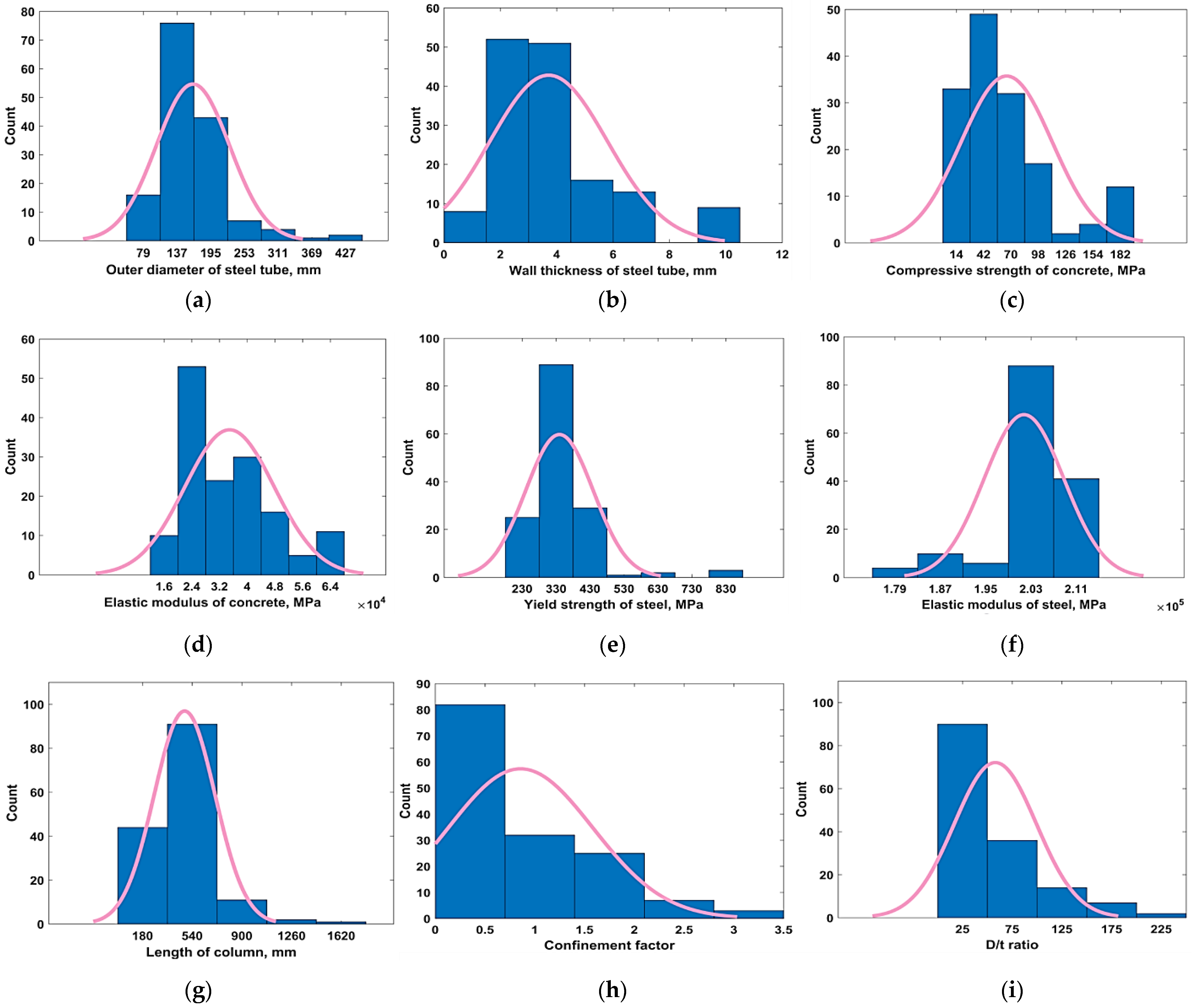
Figure 1. Frequency histograms of input variables. (a) Elastic modulus of concrete, (b) wall thickness of steel tube, (c) compressive strength of concrete, (d) Elastic modulus of concrete, (e) Yield strength of steel, (f) Elastic modulus of steel, (g) Length of column, (h) Confinement factor, (i) D/t, (j) L/D.
Materials 15 06969 g001aMaterials 15 06969 g001b
Figure 2. Flowchart of GEP modelling.
Materials 15 06969 g002
Figure 3. Effect of Nc on the performance of models. (a) R2, (b) RMSE, (c) MAE.
Materials 15 06969 g003
Figure 4. Effect of Hs on the performance of models. (a) R2, (b) RMSE, (c) MAE.
Materials 15 06969 g004
Figure 5. Effect of Ng on the performance of models. (a) R2, (b) RMSE, (c) MAE.
Materials 15 06969 g005aMaterials 15 06969 g005b
Figure 6. Comparison of regression slopes in the TR phase.
Materials 15 06969 g006
Figure 7. P/E ratio distribution of the best performing model T3, (a) TR phase, (b) TS phase.
Materials 15 06969 g007
Figure 8. Expression tree for the model T3 depicting the three sub expression trees.
Materials 15 06969 g008
Figure 9. Parametric analysis of input variables. (a) Outer diameter of steel tube (D), (b) wall thickness of steel tube (t), (c) compressive strength of concrete (fc’), (d) yield strength of steel (fy), (e) length of column, (L), (f) confinement factor (ζ), (g) ratio of L/D.
Materials 15 06969 g009aMaterials 15 06969 g009b
Figure 10. Sensitivity analysis of input variables.
Materials 15 06969 g010
Table 1. Summary of the previous studies in the literature pertaining to prediction of axial capacity of CFSS.
ReferenceModelNumber of Data PointsInput VariablesTesting Data Performance
R2MAE
Sarir et al. [48]GEP303fc’, L, D, fy, t0.939_
Javed et al. [49]GEP227fc’, L, D, fy, t, L/D0.980153.9
Khan et al. [54]GEP702fc’, L, D, fy, t, et, eb0.981290.36
Ngo et al. [50]SVR-GWO802fc’, L, D, fy, t, D/t0.996_
Jiang et al. [51]GEP32D, L, t, L/D, D/t, fy, Es, f’c, Ec, υ__
Jayalekshmi et al. [52]ANN633D, t, fy, fc’, L0.962_
Ahmadi et al. [53]ANN272D, t, fy, fc’, L0.801_
This studyGEP149D, t, fc’, Ec, fy, Es, L, ζ, D/t, L/D0.99108.7
Table 2. Descriptive statistics of the input variables.
Descriptive StatisticsD
(mm)
T
(mm)
fc
(MPa)
Ec
(MPa)
fy
(MPa)
Es
(MPa)
L
(mm)
ζ
D/t
(mm/mm)
L/D
(mm/mm)
Average164.383.7165.603.5 × 104339.85201,767485.070.8658.072.94
Standard Error5.170.173.821.1 × 1038.16575.8118.080.063.380.04
Standard Deviation63.092.0846.581.3 × 10499.577029220.730.7341.210.53
Sample Variance39804.3421701.66 × 108991449,401,97848,721116980
Kurtosis5.181.900.80−0.1811.502.219.120.943.030.84
Skewness1.791.401.240.832.75−1.012.321.191.780.08
Minimum600.8618.031.8 × 104186177,0001800.05171.8
Maximum45010.36193.306.6 × 104853213,00017603.222214.90
Table 3. Parameters setting for GEP algorithms.
ParametersSettings
Axial Capacity (Pu) of CFSS
Numerical constants
   Constant per gene10
Floating number
10
[−10, 10]
   Type of data
   Maximum complexity
   Ephemeral random constant
Genetic operators
   Rate of mutation0.00138
   Inversion rate0.00546
   IS transposition rate
   RIS transposition rate
1-point recombination rate0.00277
 2-point recombination rate
   Gene recombination rate
   Gene transposition rate
Table 4. Details of the different trials/models conducted to obtain optimal model.
Trial/ModelNo. of VariablesNo. of ChromosomesHead SizeNo. of GenesTR PhaseTS Phase
R2RMSEMAER2RMSEMAE
T1530830.92644.4443.60.94432.9323.9
T2750830.98236.5173.80.98205.3159.6
T37100830.99133.492.40.99162.2108.7
T48150830.98287.8198.10.97325.5221.7
T59200830.98255.1154.90.99162.3126.0
T67100930.98298.5202.10.96363.1243.8
T781001030.97389.0257.90.96358.3242.7
T871001130.93605.8373.10.84828.0501.3
T981001230.97385.1276.00.96386.0279.8
T108100840.98313.6209.90.97298.2222.7
T118100850.96443.8286.20.98288.9218.5
Table 5. Ideal values of performance indices.
IndexRange/Ideal Value
R2(0–1)/1
RMSE ( 0 ) / 0
MAE ( 0 ) / 0
Table 6. Ranking of models based on R2 and RMSE.
StatisticR2RMSEMAE
Rank1st2nd1st2nd1st2nd
TR PhaseT3T2, T5T3T2T3T5
TS PhaseT3T5T3T5T3T5
Table 7. Dataset used for parametric analysis.
Input VariablesConstant Input ParametersNo. of DataPoints
ParameterRange
D60–450t = 3.71, fc’ = 65.60, fy = 339.85, L = 485.07, ζ = 0.86, L/D = 2.9410
t0.86–10.36D = 164.34, fc’ = 65.60, fy = 339.85, L = 485.07, ζ = 0.86, L/D = 2.94
fc18.03–193.30D = 164.34, t = 3.71, fy = 339.85, L = 485.07, ζ = 0.86, L/D = 2.94
fy186–853D = 164.34, t = 3.71, fc’ = 65.60, L = 485.07, ζ = 0.86, L/D = 2.94
L180–1760D = 164.34, t = 3.71, fc’ = 65.60, fy = 339.85, ζ = 0.86, L/D = 2.94
ζ0.045–3.221D = 164.34, t = 3.71, fc’ = 65.60, fy = 339.85, L = 485.07, L/D = 2.94
L/D1.8–4.9D = 164.34, t = 3.71, fc’ = 65.60, fy = 339.85, L = 485.07, ζ = 0.86,
Publisher’s Note: MDPI stays neutral with regard to jurisdictional claims in published maps and institutional affiliations.