Article

Piston Wear Detection and Feature Selection Based on Vibration Signals Using the Improved Spare Support Vector Machine for Axial Piston Pumps

1
State Key Laboratory of High Performance Complex Manufacturing, Central South University, Changsha 410017, China
2
College of Mechanical and Electrical Engineering, Wenzhou University, Wenzhou 325000, China
*
Author to whom correspondence should be addressed.
Materials 2022, 15(23), 8504; https://doi.org/10.3390/ma15238504
Submission received: 9 November 2022 / Revised: 25 November 2022 / Accepted: 28 November 2022 / Published: 29 November 2022
(This article belongs to the Topic Research on the Mechanical Wear of Gear-Shaped Parts)
(This article belongs to the Section Manufacturing Processes and Systems)

Abstract

:
A piston wear fault is a major failure mode of axial piston pumps, which may decrease their volumetric efficiency and service life. Although fault detection based on machine learning theory can achieve high accuracy, the performance mainly depends on the detection model and feature selection. Feature selection in learning has recently emerged as a crucial issue. Therefore, piston wear detection and feature selection are essential and urgent. In this paper, we propose a vibration signal-based methodology using the improved spare support vector machine, which can integrate the feature selection into the piston wear detection learning process. Forty features are defined to capture the piston wear signature in the time domain, frequency domain, and time–frequency domain. The relevance and impact of sparsity in 40 features are illustrated through the single and multiple statistical feature analysis. Model performance is assessed and the sparse features are discovered. The maximum model testing and training accuracy are 97.50% and 96.60%, respectively. Spare features s10, s12, Ew(8), x7, Ee(5), and Ee(4) are selected and validated. Results show that the proposed methodology is applicable for piston wear detection and feature selection, with high model accuracy and good feature sparsity.

1. Introduction

Hydraulic transmission systems have been widely utilized in the aviation, aerospace, and marine industries, with the advantages of high power density and output efficiency [1,2]. Axial piston pumps are the key power components in hydraulic systems, and they can convert the rotating mechanical power into fluid power [3,4,5]. Typical structures of an axial piston pump are shown in Figure 1. Pistons are uniformly distributed around the center of the cylinder block. The swash plate and retainer drive the pistons reciprocating along the cylinder block center. The oil suction and extrusion are accomplished through the reciprocating movements. There are three friction pairs acting as bearing and sealing functions (marked with red lines in Figure 1): the slipper pair, the piston pair, and the valve plate pair. The piston pair has poor bearing and sealing functions due to the huge lateral forces from the inclined swash plate [6,7,8]. The poor performance of the piston pair may lead the piston surface to easily wear and become stuck. The piston wear is caused by surface microprotrusion; different microstructures are proposed to improve the film characteristics of the piston pair [9]. Proper materials of friction matching can decrease the piston wear; 940 stainless steel, F102 engineering plastics, and Al2O3 ceramic were used as matching materials in a water hydraulic pump [10]. Ceramic and 30Cr2MoVA materials were applied to an ultra-high-pressure pump [11]. In addition, an anti-friction coating was added to high-lead bronze, and the mechanical properties and wear mechanism of the piston pair were evaluated. Uniform distributions of lead segregations can improve the piston wear properties [12]. Therefore, piston wear fault detection is of great significance for the system’s efficiency and lifetime.
Numerous types of research have been carried out for the fault detection of an axial piston pump based on vibration signals. Methods based on cluster analysis [13], particle swarm optimization [14], artificial neural networks [15], hidden semi-Markov [16], and deep belief networks [17,18] are proposed, and features in the time domain (TD), frequency domain (FD), and time–frequency domains (TFD), including kurtosis, the root mean square, the energy ratio, the coefficients of the wavelet packet transform (WPT), and spectral entropy, are used as model indicators.
Although fault detection based on machine learning theory can achieve satisfactory accuracy, the performance is heavily dependent on model and feature selection [19]. Gaussian process regression (GPR), extreme gradient boosting, and support vector machine (SVM) are used for modeling the specific heat capacity in the application of solar energy [20]. Linear discriminant analysis, logistic regression, decision tree, random forest, Light-GBM, and multi-layer perceptron are utilized for the anomaly detection of the hydraulic system [21]. The GPR and support vector regression (SVR) are employed to predict the energy storage properties [22]. In addition, the convolutional neural network is proposed for the fault diagnosis of axial piston pumps [23]. Among the machine learning methods, SVM, with powerful generalization ability and high learning efficiency, has been widely used as a fault detection model for bearings [24,25,26], motors [27], gearboxes [28,29], and pumps [30]. Improved algorithms for SVM include the wavelet transform-based SVM [31], least squares-based SVM [32,33], hyper-sphere-structured SVM [34], proximal SVM [35], etc. In addition, feature selection in learning has recently emerged as a crucial issue [36,37]. Various forms of regularization are presented for feature selection during the machine learning process. The 2 regularization is not enforced, and the results of the feature selection are poor. Numerous types of research based on the 1 form, 1/2 form, and 1 + 2 form have emerged to induce sparsity for feature selection in learning [38]. The 1 regularization is widely utilized to select features during the machine learning process.
The model and feature selection during the fault detection of axial piston pumps are mostly based on expert knowledge. However, the relevance and impact of sparsity in model features are unclear. A piston wear fault is a major failure mode of axial piston pumps, but recent studies are not specific to piston wear detection and feature selection. The classical SVM is unable to complete feature selection during the learning process. In the presented study, a methodology using the improved SPARE-SVM is proposed for piston wear detection and feature selection for the first time. This methodology has the ability to integrate feature selection during the machine learning process. A large set of features is employed in the TD, FD, and TFD. The relevance and impact of sparsity in these features are illustrated through single and multiple statistical feature analysis, model performance evaluation, and feature selection analysis.

2. Materials and Methods

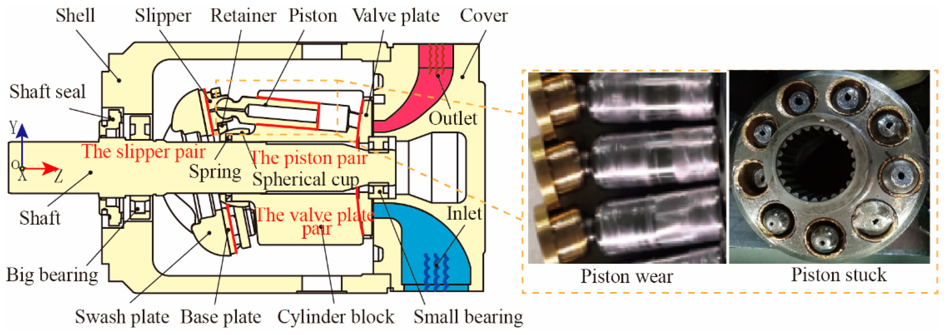
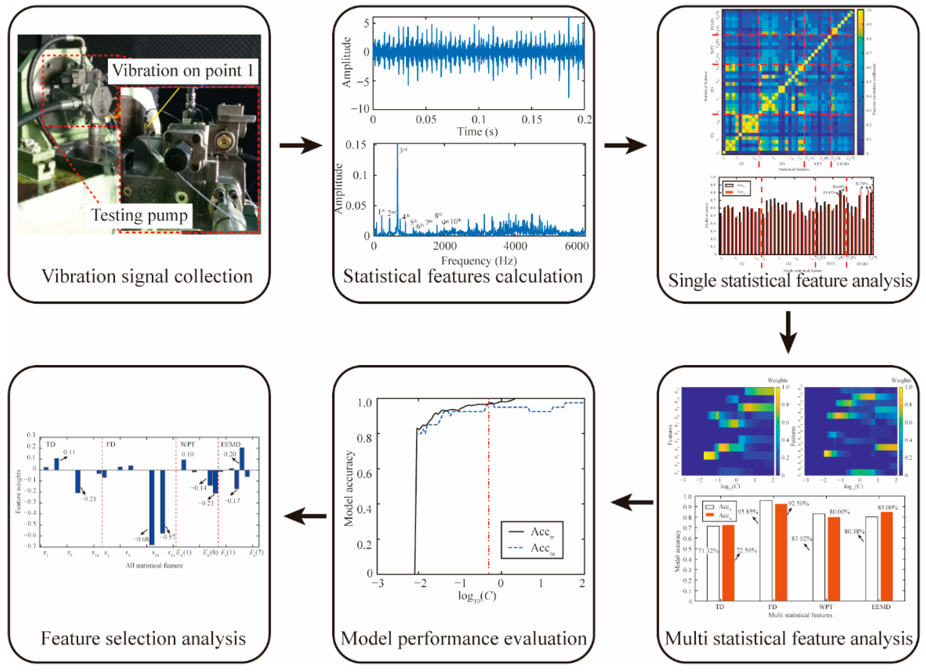
2.1. Experimental Setup and Procedure

Testing pumps are axial piston pumps with swash-plate-type variable control. Detailed parameters are shown in Table 1. The testing pump has nine pistons. The materials of the piston pair are 38CrMoAl and CuPb15Sn5. The piston diameter is 17 mm. Large fitting clearance of the piston pair will increase the leakage, while small fitting clearance may lead to the piston becoming stuck. The normal fitting clearance between the piston and the cylinder for the testing pump is approximately 0.03 mm. A piston wear fault leads to the fitting clearance exceeding the level of tolerance. Abnormal vibrations will occur simultaneously. In this paper, additional clearance is processed through the centerless grinder to simulate the piston wear fault. As shown in Figure 2, the diameter of the three marked pistons (A, B, and C) is reduced by 0.03 mm.
The testing rigs for the testing pump are shown in Figure 3. The testing pump is driven by an inverter-fed motor through the drum–gear coupling. A torque–speed transducer is used to monitor the torque and rotating speed, which is located between the testing pump and motor. The frequency converter can regulate the motor rotating speed. The discharge pressure is regulated by a pressure relief valve, and its maximum pressure is 35 MPa. The discharge pressure is measured by a pressure transducer and a pressure gauge. The pump output flow is measured by a flow transducer. The vibration signal is used for the piston wear fault detection and feature selection. The vibration acceleration on point 1 is collected by a piezoelectric accelerometer (Type LAN-XI 3050, Brüel & Kjær, Virum, Denmark) and data acquisition module (Type 4507-B-001, Brüel & Kjær, Virum, Denmark). The sampling frequency of vibration signals is 48,000 Hz. A high-pass filter is utilized to denoise raw vibration signals and the cut-off frequency is 7 Hz.
A testing pump with normal pistons (TPNP) and a testing pump with worn pistons (TPWP) are tested in the test rig, respectively. Vibration signals are compared in the TD, FD, and TFD. The denoised signals of the vibration acceleration on point 1 for the TPNP and TPWP are shown in Figure 4a,c, respectively. There are 9600 points (0.2 s) of the waveform in the TD. It is difficult to distinguish differences in the TD waveforms in Figure 4a,c. The signal’s inherent nature in the FD can be disclosed by Fourier transform (FT) analysis. The FT can reflect the frequency components and distribution of the vibration signal in the FD. There will be some abnormal frequencies in the signal spectra when a mechanical fault occurs. Spectra in the FD of the TPNP and TPWP are shown in Figure 4b,d, respectively. The frequency ranges from 0 Hz to 6000 Hz. Some differences in the spectrum distributions are presented. The amplitude of different harmonics is variable.
Signal comparison in the TD and FD is based on stationary signals. The frequency spectrum obtained from the FT may fluctuate with time, because the mechanical fault signal is not stationary when a fault occurs. Signal processing methods in the TFD have been proposed to analyze the non-stationary signals. These methods include the short-time Fourier transform, Wigner–Ville distribution, wavelet transform (WT), WPT, empirical mode decomposition (EMD), and ensemble empirical mode decomposition (EEMD), etc. The WT or WPT decomposes a signal into an approximated component and a detailed component. Moreover, the WPT has high-frequency resolution power in both the low and high frequency range, because this transform can choose the matched frequency band adaptively. A signal can be divided into a series of IMFs and a residue by the EMD or EEMD algorithm. Furthermore, the EEMD algorithm is able to overcome the mode mixing issue by adding white noise with a finite amplitude and obtain better performance. Therefore, apart from signal comparisons in the TD and FD, TFD analyses based on the WPT and EEMD algorithms are conducted on the denoised vibration signals. The wavelet is sym4 and the decomposition level is 3 for the WPT algorithm. The WPT-reconstructed coefficients of the TPNP and TPWP are shown in Figure 5. The maximum amplitude of the fifth frequency sub-band of the TPNP is approximately 2, while the maximum amplitude of the fifth frequency sub-band of the TPWP is approximately 4. The maximum amplitude of the sixth frequency sub-band of the TPNP is approximately 5, while the maximum amplitude of the sixth frequency sub-band of the TPWP is approximately 4. In addition, there are also some differences in the waveforms of the WPT-reconstructed coefficients.
For the EEMD algorithm, the ratio of the standard deviation for the added sample noise is 0.2. The ensemble number is 50 and the IMF number is 7. The EEMD IMFs of the TPNP and TPWP are shown in Figure 6. The maximum amplitude of the seventh IMF of the TPNP is approximately 0.05, while the maximum amplitude of the seventh IMF of the TPWP is approximately 0.1. In addition, there are also some differences in the waveforms of the IMFs.
Results show that some differences in the TD, FD, and TFD can be found when the pump has a piston wear fault. These differences are caused by the waveform distortions and spectrum energy relocation. Therefore, it is feasible to detect the piston wear fault through the vibration signal. This paper proposes an improved SPARE-SVM-based methodology for the piston wear detection and feature selection of axial piston pumps. The training dataset contains 220 samples of the TPNP and 45 samples of the TPWP, and the testing dataset includes 30 samples of the TPNP and 10 samples of the TPWP. The length of a single sample is 512 data points. The training and testing samples are independent of each other.

2.2. Improved SPARE-SVM Based Methodology

The SVM algorithm has been widely used in various applications, with the advantages of uncomplicated principles, easy calculation, and high classification accuracy. This algorithm aims to construct a separating hyper-plane. The hyper-plane is able to divide the dataset (xi, i = 1, 2, ∙∙∙, N) into two classes (yi = ±1). The maximum distance between the upper and lower boundary of the hyper-plane is called the maximized margin. The support vectors are data points located on the hyper-plane. The separating hyper-plane of the SVM algorithm is constructed by structural risk minimization [25].
f ( x ) = ω T x + b .
The optimal hyper-plane is built from parameters (ω, b), and estimations of the parameters are calculated as
( ω ^ , b ^ ) arg min 1 2 ω 2 2 + C n = 1 N H ω , b ( x i , y i ) ,
where parameter ω is an N-dimensional vector and parameter b is a scalar. ‖ω2 is the 2 form of the parameter ω. H(~) represents the hinge loss function of the ith data (xi, yi). The weight of H(~) is adjusted by parameter C.
H ω , b ( x i , y i ) = max { 0 , 1 y i ( ω T x i + b ) } ,
The classical SVM algorithm is unable to complete the feature selection during the machine learning process, due to the fact that the 2 form of the parameter ω is used. In addition, imbalanced datasets of two classes (yi = ±1) may also decrease the parameter sparsity and model accuracy. Therefore, the improved SPARE-SVM algorithm is put forward, using the 1 regularization form, the square hinge loss function H2(~), and the weights of the imbalanced datasets [39]. This algorithm can integrate the feature selection into the fault detection learning process.
The 1 norm can impose the sparsity of parameter ω. Meanwhile, it renders the solution of the optimal hyper-plane difficult as the 1 norm is not differentiable. The square hinge loss function H2(~) is able to deal with the non-differentiable problem of the 1 norm and solve the optimal hyper-plane. The weights of the imbalanced datasets are imposed to increase the robustness and precision of the models. Parameter estimations of the improved SPARE-SVM algorithm are calculated as follows:
( ω ^ , b ^ ) arg min ω 1 + C n = 1 N 1 H ω , b 2 ( x i , y i ) + C N 1 N + 1 n = 1 N + 1 H ω , b 2 ( x i , y i ) ,
where N−1 is the number of the class (yi = −1) and N+1 refers to the number of the other class (yi = +1).
The 1 regularization norm of parameter ω is non-differentiable. The forward–backward splitting algorithm can solve this optimization problem using the gradient descent step of the square hinge loss function H2(~). The proximity operator of parameter ω is defined as
Prox { 1 norm [ ω ( 1 ) ] } = argmin 1 2 ω ( 1 ) ω 2 2 + 1 norm [ ω ( 1 ) ] ,
where ω(1) is the parameter estimation of the 1 regularization norm. The parameter ω is obtained by the iterative calculation of the forward-backward splitting algorithm.
ω ( z ) = Prox { ω ( z 1 ) 1 D H ω ( z 1 ) , b 2 ( x i , y i ) } ,
where ω(z) and ω(z − 1) are the parameter estimations of the zth and z − 1th iterative. The parameter D is a constant of gradient descent order, and ∇H2(~) refers to the Lipschitz-continuous gradient of the square hinge loss function.
The improved SPARE-SVM-based methodology is proposed for the piston wear detection and feature selection of axial piston pumps. The flowchart of this methodology is shown in Figure 7. First, the vibration signals of the axial piston pump are collected by the data acquisition module. Second, a comprehensive set of features is defined in the TD, FD, and TFD. Third, single statistical feature analysis is conducted to investigate the feature correlations and model performance obtained from a single feature. Fourth, multiple statistical feature analysis is used to illustrate the weight variations and model performance of multiple features in the TD, FD, and TFD. Fifth, the weight variations and model accuracy of the large set of features are analyzed through the model performance evaluation. Lastly, feature selection analysis is utilized to validate the feature sparsity.
Differences in the waveforms in the TD, FD, and TFD are shown through the signal comparison in Section 2.1. Statistical feature calculation in the TD [40,41], FD [42], and TFD [43,44] is conducted, and 40 features are constructed to capture the fault characteristics from different aspects.
Statistical features used in the TD are listed in Table 2, where xi (i = 1, 2, …, 11) denotes the ith feature, x(n) (n = 1, 2, …, N) refers to the TD signal, and N is the data length of the vibration signal. The mean value and standard deviation (x1 and x2) reflect the average and deviation of the TD signal. The root amplitude, root mean square, and peak value (x3, x4, and x5) refer to the signal amplitude and energy. The skewness (x6) measures the data asymmetry around the mean value. The kurtosis (x7) shows the outlier proneness of a distribution. The crest factor (x8) and clearance factor (x9) indicate peak severity. The shape factor (x10) reveals the shape of the distribution. The impulse factor (x11) detects the impulse components of the distribution.
Statistical features in the FD are shown in Table 3, where si (i = 1, 2, …, 14) denotes the ith feature, s(k) (k = 1, 2, …, K) is the amplitude and f(k) (k = 1, 2, …, K) represents the corresponding frequency for the kth FT spectrum line, and K refers to the FT spectrum line number. The mean frequency (s1) reflects the signal energy in the FD. The frequency center, root 2 order weighting, root 4-2 order weighting, 2-4-order weighting, 2 order center moment, 3 order center moment, 4 order center moment, and root 2 order center moment (s2, s3, s4, s5, s6, s7, s8, and s9) refer to the main frequency position changes in the frequency spectrum. The root 2 order convergence index, 3 order convergence index, 4 order convergence index, 1/2 order convergence index, and root 2 order convergence index (s10, s11, s12, s13, and s14) reveal the convergence characteristics of the frequency spectrum power.
Signal features obtained from the TFD are effective compensations for the statistical features in the TD and FD. The energy ratio of the frequency sub-bands decomposed by the WPT and the energy ratio of the IMFs decomposed by the EEMD are used as statistical features in the TFD. As shown in Table 4, Ew(i) (i = 1, 2, …, 2m) denotes the ith frequency sub-band feature of the WPT, xi(j) refers to the ith frequency sub-band, and m represents the decomposition level (m = 3). For the EEMD algorithm, Ee(i) (i = 1, 2, …, L) denotes the ith IMF feature, ci(j) refers to the ith IMF, and L represents the number of IMFs (L = 7).

3. Results and Discussion

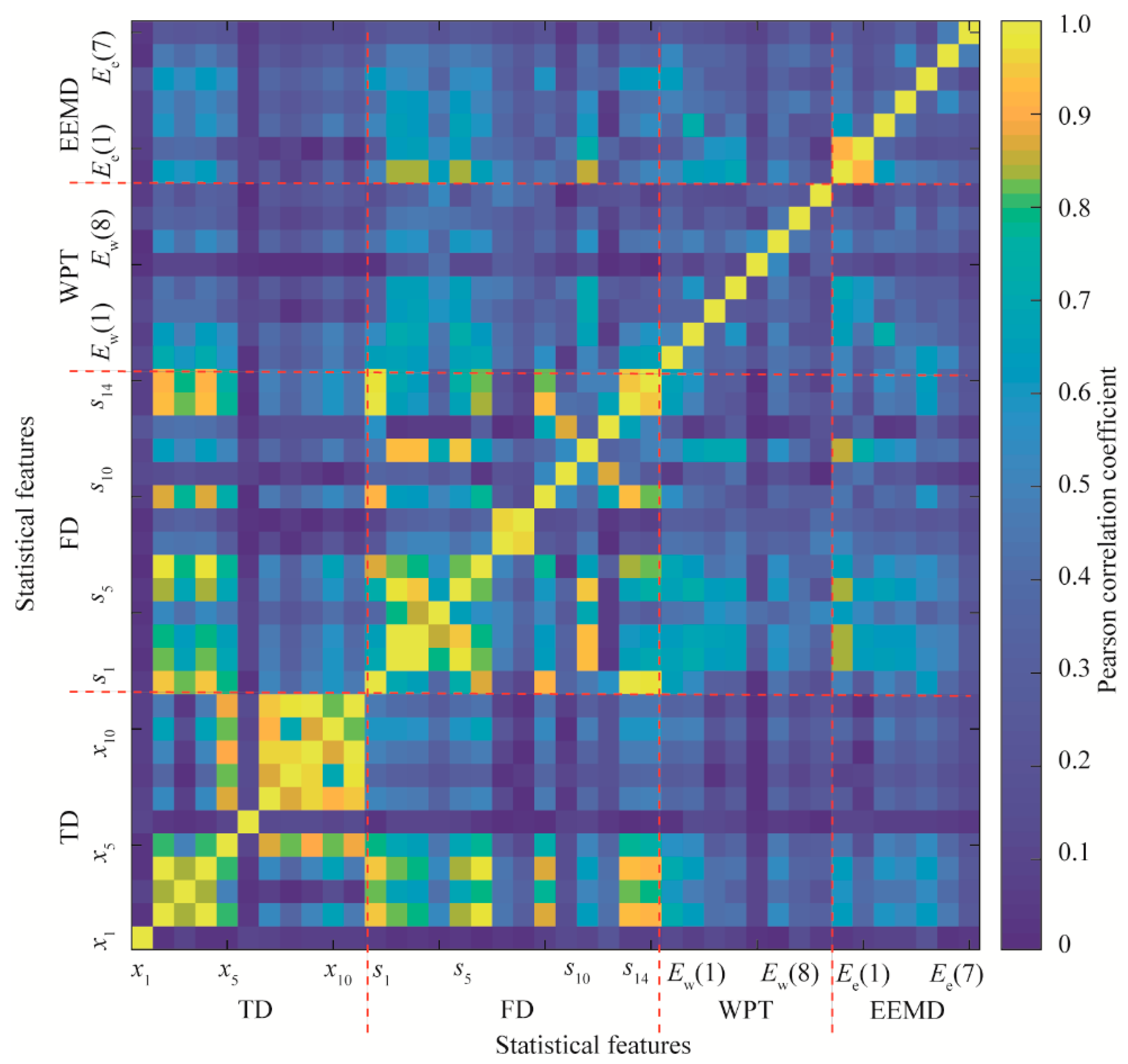
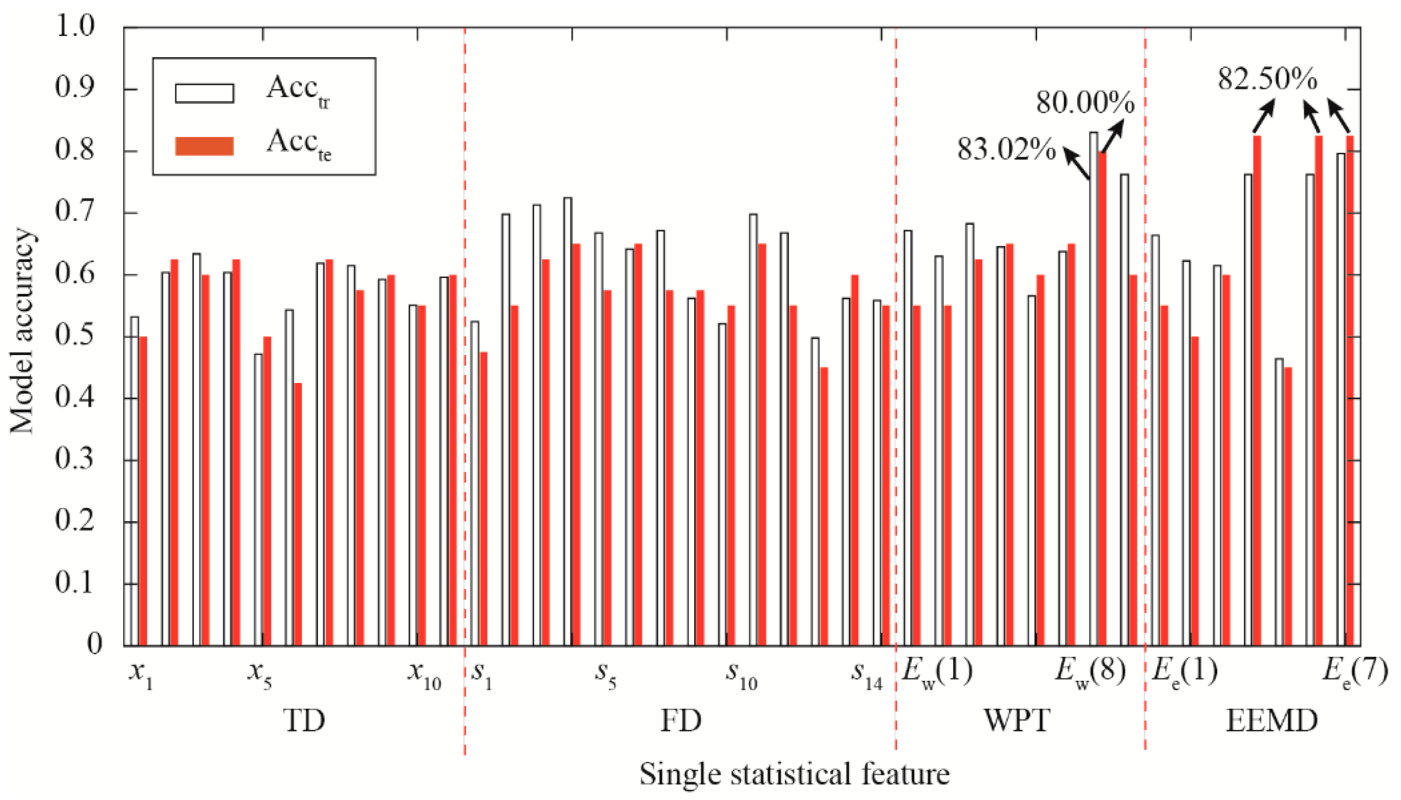
3.1. Single Statistical Feature Analysis

Statistical feature correlations and model performance obtained from the single feature were investigated via single statistical feature analysis. The correlation analysis of the features of all training samples was carried out. The absolute values of the Pearson correlation coefficients (PCCs) are shown in Figure 8. The diagonal entries are only 1 due to the fact that all statistical features are always directly correlated to themselves. Statistical features in the TD or FD have a strong correlation. For example, the root mean square (x4) is directly correlated to the standard deviation (x2) as the PCC is 1. The PCCs between x9 and x8, x7 are 0.954 and 0.959, respectively. The PCCs between x11 and x9, x8, x7 are 0.996, 0.977, and 0.946, respectively.
In terms of the features in the FD, the PCC between s3 and s2 is 0.993. The PCCs between s5 and s3, s2 equal 0.952 and 0.977, respectively. The PCC between s8 and s7 is 0.954. The PCC between s9 and s1 equals 0.920. The PCCs between s11 and s5, s3, s2 are 0.940, 0.926, and 0.924, respectively. The PCCs between s13 and s9, s1 equal 0.933 and 0.986, respectively. The PCCs between s14 and s13, s1 are 0.951 and 0.970, respectively.
Moreover, some statistical features in the FD are highly correlated to those in the TD. For instance, the PCCs between s1 and x4, x2 equal 0.943. The PCCs between s6 and x4, x2 equal 0.976. The PCCs between s13 and x4, x2 equal 0.930. The PCCs between s14 and x4, x2 equal 0.915. Strong correlations are due to the fact that the calculation processes of some statistical features in the TD and FD are related to each other.
In terms of statistical features in the TFD, most features calculated by the WPT and EEMD have a lower correlation with each other due to frequency decompositions of the vibration signals. Therefore, statistical features with lower correlations in the TFD have better independence than features in the TD or FD.
A single statistical feature is utilized as a model indicator for piston wear detection. The model accuracy of the training dataset (Acctr) and the testing dataset (Accte) is shown in Figure 9. Features Ee(4), Ee(6), and Ee(7) in the TFD yield better testing performance, with Accte of 82.50%. Feature Ew(7) has the best training performance, with the maximum Acctr of 83.02%. Moreover, the Accte of this single feature equals 80.00%. In addition, most features in the FD have better model accuracy than features in the TD. Features, s2, s3, s4, s5, s6, s7, s10, and s11 in the FD have larger Acctr values than features in the TD. A single feature of the energy ratio is able to capture the piston wear information. Results of the single statistical feature analysis show that a single feature in the TFD has better independence and model accuracy.

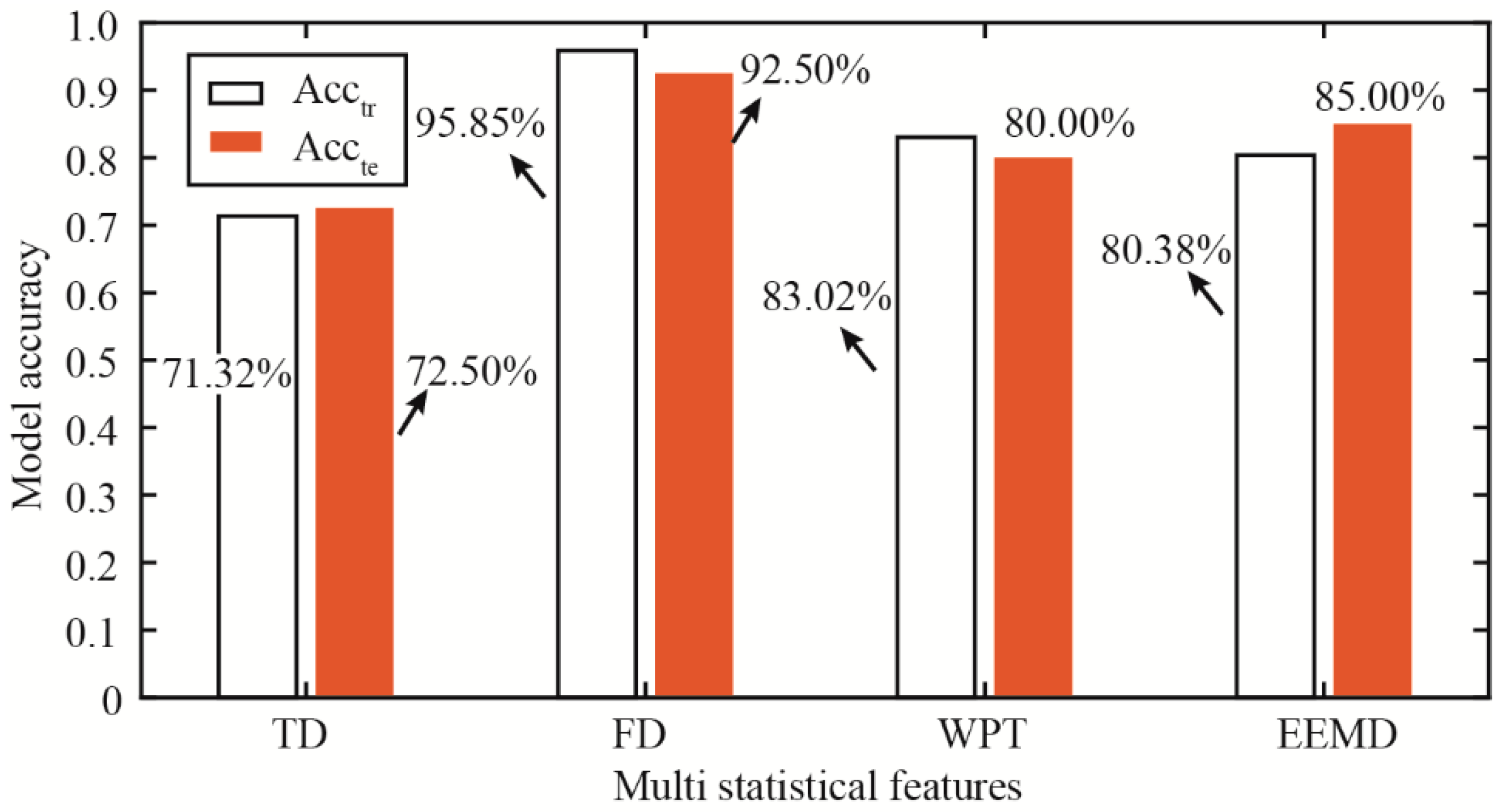
3.2. Multiple Statistical Feature Analysis

Weight variations of multiple features in the TD, FD, and TFD are shown in Figure 10. Abscissas are the logarithmic coordinates of parameter C. The parameter C ranges from 1.00 × 10⁻³ to 1.00 × 10², and it can adjust the weights of the square hinge loss function H2(~). Vertical coordinates refer to feature weights varying with parameter C during the piston wear detection process. Figure 10a shows that features x3, x4, x7, and x8 are the four first features selected by the multiple statistical feature analysis using the improved SPARE-SVM algorithm. These features are excluded as C increases. For features (x7, x8, x9, and x11), with strong correlations in the TD, only features x9 and x11 remain included when increasing parameter C. As shown in Figure 10b, features s5, s11, and s13 are selected among the multiple correlated features in the FD. Weight variations of multiple features calculated by the WPT are shown in Figure 10c. Ew(7) and Ew(8) are selected as the two first features and they remain included during the piston wear detection process. The three first selected features from the EEMD are Ee(4), Ee(5), and Ee(6), as shown in Figure 10d, and they continue to be selected as parameter C increases.
Multiple statistical features calculated from the TD, FD, WPT, and EEMD are employed as model indicators for piston wear detection, respectively. Moreover, the model accuracy Acctr and Accte is shown in Figure 11. Multiple features in the FD have the maximum model accuracy, where Acctr and Accte are 95.85% and 92.50%, respectively. Features in the TD have the minimum model accuracy, where Acctr and Accte are 71.32% and 72.50%, respectively. The Acctr and Accte for the WPT are 83.02% and 80.00%, respectively. Moreover, the Acctr and Accte for the EEMD are 80.38% and 85.00%, respectively. The model accuracy of multiple statistical features in the TFD is larger than that of features in the TD. Results show that piston wear detection based on multiple statistical features in the TD is not applicable. Features in the FD and TFD are effective compensations for the detection model. The model accuracy of features in the FD and TFD is higher and satisfactory.

3.3. Model Performance Evaluation

The large set of features in the TD, FD, and TFD is used as the input of the improved SPARE-SVM model for piston wear detection simultaneously. All feature weights varying with parameter C during the model learning process are shown in Figure 12a. All statistical features are excluded when parameter C is smaller than 9.11 × 10⁻³. The energy ratio features Ew(7), Ew(8), and Ee(4) are the three first features selected due to the high independence and model accuracy, and they are shown in Figure 8 and Figure 9, respectively. These variations are verified with the results of the multiple statistical feature analysis shown in Figure 10c,d. Most statistical features calculated from the TD, WPT, and EEMD have decreasing weights when parameter C continues to increase. The weights of some statistical features (s1, s10, s12, and s13) in the FD increase as parameter C increases. They agree with the results shown in Figure 10b.
The model accuracy Acctr and Accte varying with parameter C during the model learning process is shown in Figure 12b. There is a sudden change in the model accuracy when C is around 9.11 × 10⁻³. The change is due to the fact that a large set of features in the TD, FD, and TFD is not selected during the model learning process when C is less than 9.11 × 10⁻³. The Accte increases as parameter C increases. The maximum value of the Accte of 97.50% occurs when C is around 4.75 × 10⁻¹. Moreover, the Acctr is 96.60% at this time. The Accte is no longer improved as parameter C increases. In addition, when C is larger than 6.00 × 10⁻¹, the Accte begins to decline. The model accuracy Acctr gradually increases as parameter C becomes larger, which means that over-fitting occurs in the model learning process. It is found that the parameter C is able to regulate the trade-off between the feature sparsity and model accuracy. Therefore, the optimal parameter C is chosen as 4.75 × 10⁻¹ through the model performance evaluation. It is found that the model accuracy for all features is higher than that obtained from the single and multiple statistical feature analysis. This means that the model accuracy for all features is more satisfactory.

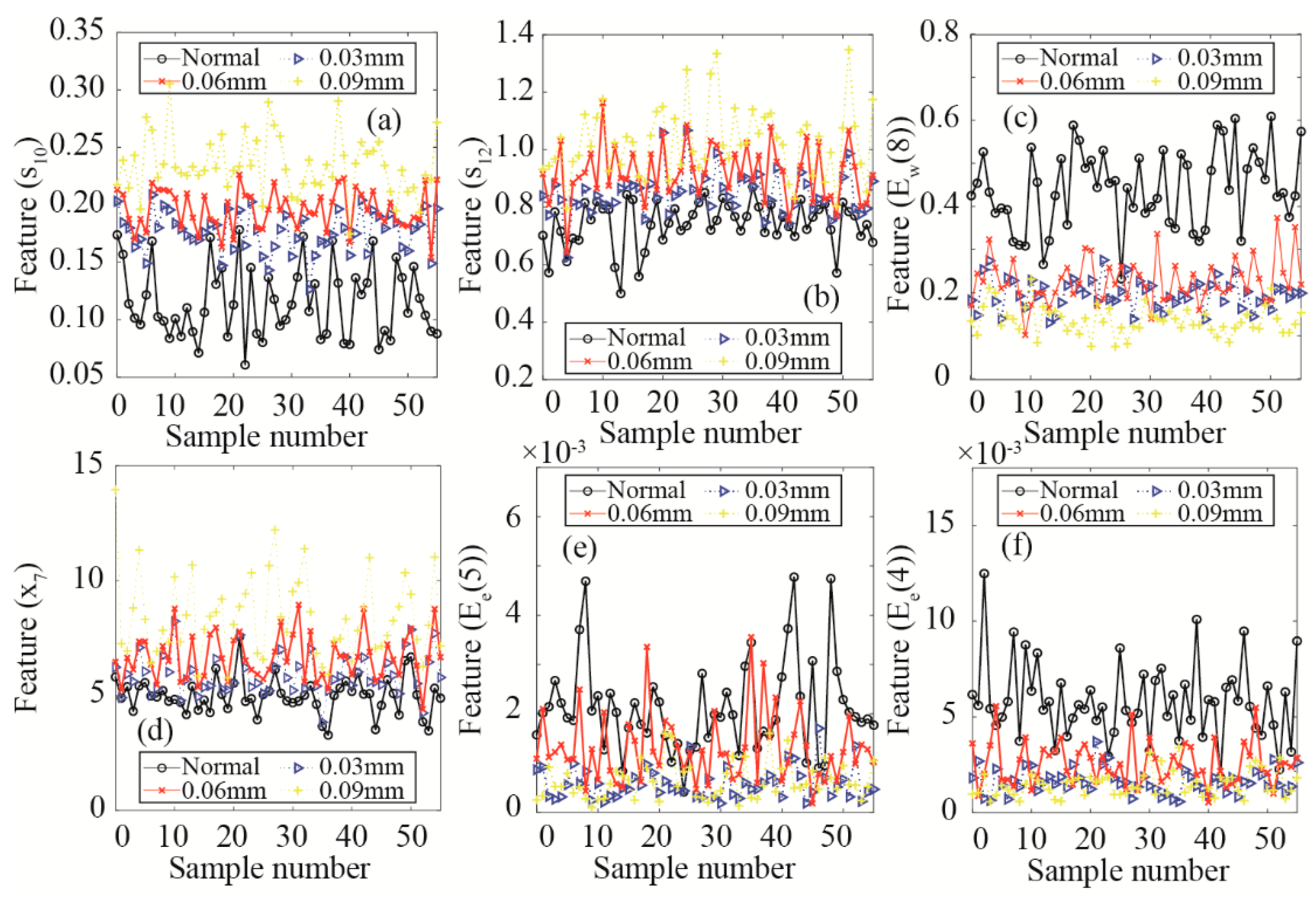
3.4. Feature Selection Analysis

Considering that the classical SVM algorithm cannot complete the feature selection during the machine learning process, the feature selection analysis is only conducted based on the improved SPARE SVM algorithm. The weights of the large set of features in the TD, FD, and TFD with C = 4.75 × 10⁻¹ are shown in Figure 13. Statistical features x1, x3, x7, x11, s1, s4, s6, s10, s12, Ew(2), Ew(4), Ew(7), Ew(8), Ee(1), Ee(3), Ee(4), Ee(5), and Ee(6) are selected by the improved SPARE-SVM algorithm. Meanwhile, features x2, x4, x5, x6, x8, x9, x10, s2, s3, s5, s7, s8, s9, s11, s13, s14, Ew(1), Ew(3), Ew(5), Ew(6), Ee(2), and Ee(7) are excluded with no weights. Features s10 and s12 in the FD have larger weights than other features. The weights of s10 and s12 are −0.68 and −0.57, respectively. The weights of the features x3 and x7 in the TD are 0.11 and −0.21, respectively. The weights of the features Ew(2), Ew(7), and Ew(8) calculated by the WPT are 0.10, −0.14, and −0.21, respectively. The weights of the features Ee(4) and Ee(5) calculated by the EEMD are −0.17 and 0.20, respectively. The order of the first six sparse features is s10, s12, Ew(8), x7, Ee(5), and Ee(4).
Different cases of additional clearance (0.03 mm, 0.06 mm, and 0.09 mm) are investigated to validate the six sparse features selected by the improved SPARE-SVM algorithm for piston wear detection. Feature comparisons under different cases of piston wear are shown in Figure 14. The abscissa is the sample number, and the sparse features of 55 samples are calculated. As shown in Figure 14a,b, different wear cases affect the convergence characteristics of the frequency spectrum power, especially for the root 2 order convergence index (s10) and 4 order convergence index (s12,). The indexes s10 and s12 become larger as the clearance increases. The case of the normal piston can be identified from the energy ratio features Ew(8), Ee(5), and Ee(4), as shown in Figure 14c,e,f, respectively. The case of 0.09 mm is different from the other three cases in terms of kurtosis (x7). The six major sparse features of the piston wear fault are s10, s12, Ew(8), x7, Ee(5), and Ee(4) due to the weight differences. Results show that the improved SPARE-SVM model is effective for piston wear fault detection and sparse feature selection.

4. Conclusions

This paper proposes a methodology using the improved SPARE-SVM for piston wear detection and feature selection for the first time. An experimental investigation was carried out, and the following conclusions were drawn.
  • The proposed methodology can integrate feature selection during the machine learning process of piston wear detection.
  • A large set of features is constructed in the TD, FD, and TFD. Single and multiple feature analysis are utilized to illustrate the relevance and impact of sparsity in the comprehensive set of features.
  • Feature effects on the model accuracy are analyzed. The maximum model testing and training accuracy values are 97.50% and 96.60%, respectively.
  • Spare features s10, s12, Ew(8), x7, Ee(5), and Ee(4) are selected and validated.
Future work will focus on the improvement of the SPARE-SVM algorithm. Then, this improved algorithm will be used for other types of fault detection in axial piston pumps.

Author Contributions

Conceptualization, S.X. and Y.X.; methodology, S.X.; software, S.X.; validation, S.X., Y.X. and J.X.; formal analysis, S.X.; investigation, S.X.; resources, Y.X.; data curation, S.X.; writing—original draft preparation, S.X.; writing—review and editing, S.X.; visualization, S.X.; supervision, Y.X.; project administration, J.X.; funding acquisition, Y.X. All authors have read and agreed to the published version of the manuscript.

Funding

This research was funded by the National Natural Science Foundation of China (Grant No. 52105078), the Project of State Key Laboratory of High Performance Complex Manufacturing (Grant No. ZZYJKT2021-16), and the Open Foundation of the State Key Laboratory of Fluid Power and Mechatronic Systems (Grant No. GZKF-202007).

Institutional Review Board Statement

Not applicable.

Informed Consent Statement

Not applicable.

Data Availability Statement

The data presented in this study are available on request from the corresponding author. The data are not publicly available due to an ongoing study.

Acknowledgments

The authors would like to thank Zhihua Ye, Huaijun Shi, and Ping Wu, from Ningbo Hilead Hydraulic Co., Ltd., for their help in preparing the pumps and performing the tests.

Conflicts of Interest

The authors declare no conflict of interest.

References

  1. Tang, S.; Zhu, Y.; Yuan, S. Intelligent fault diagnosis of hydraulic piston pump based on deep learning and Bayesian optimization. ISA Trans. 2022, 129 Pt A, 555–563. [Google Scholar] [CrossRef]
  2. Zhang, C.C.; Zhu, C.H.; Meng, B.; Li, S. Challenges and Solutions for High-Speed Aviation Piston Pumps: A Review. Aerospace 2021, 8, 392–398. [Google Scholar] [CrossRef]
  3. Xiao, C.; Tang, H.; Ren, Y.; Xiang, J.; Kumar, A. Adaptive MOMEDA based on improved advance-retreat algorithm for fault features extraction of axial piston pump. ISA Trans. 2022, 128 Pt B, 503–520. [Google Scholar] [CrossRef]
  4. Zhao, B.; Hu, X.; Li, H.; Liu, Y.; Zhang, B.; Dong, Q. A New Approach for Modeling Mixed Lubricated Piston-Cylinder Pairs of Variable Lengths in Swash-Plate Axial Piston Pumps. Materials 2021, 14, 5836–5841. [Google Scholar] [CrossRef] [PubMed]
  5. Xia, S.Q.; Xia, Y.M.; Xiang, J.W. Modelling and Fault Detection for Specific Cavitation Damage Based on the Discharge Pressure of Axial Piston Pumps. Mathematics 2022, 10, 2461–2469. [Google Scholar] [CrossRef]
  6. Chao, Q.; Zhang, J.H.; Xu, B.; Wang, Q.N.; Lyu, F.; Li, K. Integrated slipper retainer mechanism to eliminate slipper wear in high-speed axial piston pumps. Front. Mech. Eng. 2022, 17, 1. [Google Scholar] [CrossRef]
  7. Li, Y.; Chen, X.; Luo, H.; Zhang, J. An Empirical Model for the Churning Losses Prediction of Fluid Flow Analysis in Axial Piston Pumps. Micromachines 2021, 12, 398–402. [Google Scholar] [CrossRef] [PubMed]
  8. Chao, Q.; Xu, Z.; Tao, J.; Liu, C. Capped piston: A promising design to reduce compressibility effects, pressure ripple and cavitation for high-speed and high-pressure axial piston pumps. Alex. Eng. J. 2023, 62, 509–521. [Google Scholar] [CrossRef]
  9. Qi, B.; Yong, Z. Tribological study of piston–cylinder interface of radial piston pump in high-pressure common rail system considering surface topography effect. Proc. Inst. Mech. Eng. Part J J. Eng. Tribol. 2019, 234, 1381–1395. [Google Scholar] [CrossRef]
  10. Huayong, Y.; Jian, Y.; Hua, Z. Research on materials of piston and cylinder of water hydraulic pump. Ind. Lubr. Tribol. 2003, 55, 38–43. [Google Scholar] [CrossRef]
  11. Zhang, J.; Qiu, X.; Gong, X.; Kong, X. Wear behavior of friction pairs of different materials for ultra-high-pressure axial piston pump. Proc. Inst. Mech. Eng. Part E J. Process Mech. Eng. 2018, 233, 945–953. [Google Scholar] [CrossRef]
  12. D’Andrea, D.; Epasto, G.; Bonanno, A.; Guglielmino, E.; Benazzi, G. Failure analysis of anti-friction coating for cylinder blocks in axial piston pumps. Eng. Fail. Anal. 2019, 104, 126–138. [Google Scholar] [CrossRef]
  13. Gao, Q.; Xiang, J.W.; Hou, S.M.; Tang, H.S.; Zhong, Y.T.; Ye, S.G. Method using L-kurtosis and enhanced clustering-based segmentation to detect faults in axial piston pumps. Mech. Syst. Signal Process. 2021, 147, 107130. [Google Scholar] [CrossRef]
  14. Chaoang, X.; Hesheng, T.; Yan, R. Compressed sensing reconstruction for axial piston pump bearing vibration signals based on adaptive sparse dictionary model. Meas. Control 2020, 53, 649–661. [Google Scholar] [CrossRef] [Green Version]
  15. Maradey Lázaro, J.G.; Borrás Pinilla, C. A methodology for detection of wear in hydraulic axial piston pumps. Int. J. Interact. Des. Manuf. 2020, 14, 1103–1119. [Google Scholar] [CrossRef]
  16. Dong, M.; He, D. A segmental hidden semi-Markov model (HSMM)-based diagnostics and prognostics framework and methodology. Mech. Syst. Signal Process. 2007, 21, 2248–2266. [Google Scholar] [CrossRef]
  17. Wang, S.H.; Xiang, J.W.; Zhong, Y.T.; Tang, H.S. A data indicator-based deep belief networks to detect multiple faults in axial piston pumps. Mech. Syst. Signal Process. 2018, 112, 154–170. [Google Scholar] [CrossRef]
  18. Hou, X.; Guo, W.; Ren, S.; Li, Y.; Si, Y.; Su, L. Bolt-Loosening Detection Using 1D and 2D Input Data Based on Two-Stream Convolutional Neural Networks. Materials 2022, 15, 6757–6762. [Google Scholar] [CrossRef]
  19. Li, H.; Tian, S.; Yang, Z. A Novel Blade Vibration Monitoring Experimental System Based on Blade Tip Sensing. Materials 2022, 15, 6987–6995. [Google Scholar] [CrossRef] [PubMed]
  20. Said, Z.; Sharma, P.; Elavarasan, R.M.; Tiwari, A.K.; Rathod, M.K. Exploring the specific heat capacity of water-based hybrid nanofluids for solar energy applications: A comparative evaluation of modern ensemble machine learning techniques. J. Energy Storage 2022, 54, 105230. [Google Scholar] [CrossRef]
  21. Kim, D.; Heo, T.Y. Anomaly Detection with Feature Extraction Based on Machine Learning Using Hydraulic System IoT Sensor Data. Sensors 2022, 22, 2479. [Google Scholar] [CrossRef] [PubMed]
  22. Said, Z.; Sharma, P.; Aslfattahi, N.; Ghodbane, M. Experimental analysis of novel ionic liquid-MXene hybrid nanofluid’s energy storage properties: Model-prediction using modern ensemble machine learning methods. J. Energy Storage 2022, 52, 104858. [Google Scholar] [CrossRef]
  23. Tang, S.; Yuan, S.; Zhu, Y.; Li, G. An Integrated Deep Learning Method towards Fault Diagnosis of Hydraulic Axial Piston Pump. Sensors 2020, 20, 6576. [Google Scholar] [CrossRef] [PubMed]
  24. Cui, M.L.; Wang, Y.Q.; Lin, X.S.; Zhong, M.Y. Fault Diagnosis of Rolling Bearings Based on an Improved Stack Autoencoder and Support Vector Machine. IEEE Sens. J. 2021, 21, 4927–4937. [Google Scholar] [CrossRef]
  25. Wang, Z.; Yao, L.; Chen, G.; Ding, J. Modified multiscale weighted permutation entropy and optimized support vector machine method for rolling bearing fault diagnosis with complex signals. ISA Trans. 2021, 114, 470–484. [Google Scholar] [CrossRef]
  26. Kecik, K.; Smagala, A.; Lyubitska, K. Ball Bearing Fault Diagnosis Using Recurrence Analysis. Materials 2022, 15, 5940–5952. [Google Scholar] [CrossRef] [PubMed]
  27. Lu, L.; Wang, W. Fault Diagnosis of Permanent Magnet DC Motors Based on Multi-Segment Feature Extraction. Sensors 2021, 21, 7505. [Google Scholar] [CrossRef]
  28. Dhiman, H.; Deb, D.; Muyeen, S.M.; Kamwa, I. Wind Turbine Gearbox Anomaly Detection Based on Adaptive Threshold and Twin Support Vector Machines. IEEE Trans. Energy Convers. 2021, 36, 3462–3469. [Google Scholar] [CrossRef]
  29. Gelman, L.; Solinski, K.; Ball, A. Novel Instantaneous Wavelet Bicoherence for Vibration Fault Detection in Gear Systems. Energies 2021, 14, 6811–6820. [Google Scholar] [CrossRef]
  30. Ranawat, N.S.; Kankar, P.K.; Miglani, A. Fault Diagnosis in Centrifugal Pump using Support Vector Machine and Artificial Neural Network. J. Eng. Res. 2021, 9, 99–111. [Google Scholar] [CrossRef]
  31. Kshirsagar, P.R.; Joshi, K.A.; Hendre, V.S.; Paliwal, K.K.; Akojwar, S.G.; Atauurahman, S. Mental task classification using wavelet transform and support vector machine. Int. J. Biomed. Eng. Technol. 2021, 37, 368–381. [Google Scholar] [CrossRef]
  32. Lu, Y.; Huang, Z.P. A new hybrid model of sparsity empirical wavelet transform and adaptive dynamic least squares support vector machine for fault diagnosis of gear pump. Adv. Mech. Eng. 2020, 12, 168781402092204. [Google Scholar] [CrossRef]
  33. Chen, S.L.; Gao, Z.H.; Zhu, X.Q.; Du, Y.M.; Pang, C. Unstable unsteady aerodynamic modeling based on least squares support vector machines with general excitation. Chin. J. Aeronaut. 2020, 33, 2499–2509. [Google Scholar] [CrossRef]
  34. Wang, Y.J.; Kang, S.Q.; Jiang, Y.C.; Yang, G.X.; Song, L.X.; Mikulovich, V.I. Classification of fault location and the degree of performance degradation of a rolling bearing based on an improved hyper-sphere-structured multi-class support vector machine. Mech. Syst. Signal Process. 2012, 29, 404–414. [Google Scholar] [CrossRef]
  35. Li, G.; Yang, L.; Wu, Z.; Wu, C. D.C. Programming for sparse proximal support vector machines. Inf. Sci. 2021, 547, 187–201. [Google Scholar] [CrossRef]
  36. Ye, Z.; Yu, J.B. Multi-level features fusion network-based feature learning for machinery fault diagnosis. Appl. Soft Comput. 2022, 122, 108900. [Google Scholar] [CrossRef]
  37. Dong, W.; Zhang, S.Q.; Hu, M.F.; Zhang, L.G.; Liu, H.T. Intelligent fault diagnosis of wind turbine gearboxes based on refined generalized multi-scale state joint entropy and robust spectral feature selection. Nonlinear Dyn. 2022, 107, 2485–2517. [Google Scholar] [CrossRef]
  38. Zhang, Z.Z.; Li, S.M.; Lu, J.T.; Xin, Y.; Ma, H.J. Intrinsic component filtering for fault diagnosis of rotating machinery. Chin. J. Aeronaut. 2021, 34, 397–409. [Google Scholar] [CrossRef]
  39. Spilka, J.; Frecon, J.; Leonarduzzi, R.; Pustelnik, N.; Abry, P.; Doret, M. Sparse Support Vector Machine for Intrapartum Fetal Heart Rate Classification. IEEE J. Biomed. Health Inform. 2017, 21, 664–671. [Google Scholar] [CrossRef] [PubMed]
  40. Cao, J.; Yang, Z.; Tian, S.; Li, H.; Jin, R.; Yan, R.; Chen, X. Biprobes Blade Tip Timing Method for Frequency Identification Based on Active Aliasing Time-Delay Estimation and Dealiasing. IEEE Trans. Ind. Electron. 2022, 70, 1939–1948. [Google Scholar] [CrossRef]
  41. Tang, H.B.; Fu, Z.; Huang, Y. A fault diagnosis method for loose slipper failure of piston pump in construction machinery under changing load. Appl. Acoust. 2021, 172, 107634. [Google Scholar] [CrossRef]
  42. Zheng, Z.; Xin, G. Fault Feature Extraction of Hydraulic Pumps Based on Symplectic Geometry Mode Decomposition and Power Spectral Entropy. Entropy 2019, 21, 476–482. [Google Scholar] [CrossRef] [PubMed] [Green Version]
  43. Jiang, W.L.; Zheng, Z.; Zhu, Y.; Li, Y. Demodulation for hydraulic pump fault signals based on local mean decomposition and improved adaptive multiscale morphology analysis. Mech. Syst. Signal Process. 2015, 58–59, 179–205. [Google Scholar] [CrossRef]
  44. Gao, Z.; Lin, J.; Wang, X.; Xu, X. Bearing Fault Detection Based on Empirical Wavelet Transform and Correlated Kurtosis by Acoustic Emission. Materials 2017, 10, 571–579. [Google Scholar] [CrossRef] [PubMed]
Figure 1. Typical structure and piston wear of axial piston pumps.
Materials 15 08504 g001
Figure 2. Process of the piston wear fault.
Materials 15 08504 g002
Figure 3. Layout of the test rig.
Materials 15 08504 g003
Figure 4. Denoised signals and the FT spectra. (a) Denoised signal of the TPNP; (b) spectrum of the TPNP; (c) denoised signal of the TPWP; (d) spectrum of the TPWP.
Materials 15 08504 g004
Figure 5. WPT-reconstructed coefficients. (a) TPNP; (b) TPWP.
Materials 15 08504 g005
Figure 6. EEMD IMFs. (a) TPNP; (b) TPWP.
Materials 15 08504 g006
Figure 7. Flowchart of the improved SPARE-SVM-based methodology.
Materials 15 08504 g007
Figure 8. Correlations between statistical features.
Materials 15 08504 g008
Figure 9. Model performance obtained from single statistical feature.
Materials 15 08504 g009
Figure 10. Weight variations of multiple features. (a) TD; (b) FD; (c) WPT; (d) EEMD.
Materials 15 08504 g010
Figure 11. Model performance obtained from multiple statistical features.
Materials 15 08504 g011
Figure 12. Weight variations and model accuracy for all features. (a) Weight variations of all features; (b) model accuracy obtained from all features.
Materials 15 08504 g012
Figure 13. Weight variations of all features with C = 4.75 × 10⁻¹.
Materials 15 08504 g013
Figure 14. Six sparse feature comparisons under different cases of piston wear.
Materials 15 08504 g014
Table 1. Detailed descriptions of the testing pumps.
No.ParametersValues
1Rated speed1500 r/min
2Maximum value of the displacement40 cm3/r
3Maximum value of the discharge pressure35 MPa
4Piston diameter17 mm
5Piston number9
Table 2. Statistical features in the TD.
No.DescriptionExpressionNo.DescriptionExpression
1Mean value x 1 = 1 N n = 1 N x ( n ) 2Standard deviation x 2 = 1 N 1 n = 1 N [ x ( n ) x 1 ] 2
3Root amplitude x 3 = [ 1 N n = 1 N | x ( n ) | ] 2 4Root mean square x 4 = 1 N n = 1 N x ( n ) 2
5Peak value x 5 = max | x ( n ) | 6Skewness value x 6 = 1 ( N 1 ) x 2 3 n = 1 N [ x ( n ) x 1 ] 3
7Kurtosis value x 7 = 1 ( N 1 ) x 2 4 n = 1 N [ x ( n ) x 1 ] 4 8Crest factor x 8 = x 5 x 4
9Clearance factor x 9 = x 5 x 3 10Shape factor x 10 = N x 4 / n = 1 N | x ( n ) |
11Impulse factor x 11 = N x 5 / n = 1 N | x ( n ) |
Table 3. Statistical features in the FD.
No.DescriptionExpressionNo.DescriptionExpression
1Mean frequency s 1 = 1 K k = 1 K s ( k ) 2Frequency center s 2 = k = 1 K f ( k ) s ( k ) / k = 1 K s ( k )
3Root 2 order weighting s 3 = k = 1 K f 2 ( k ) s ( k ) / k = 1 K s ( k ) 4Root 4-2 order weighting s 4 = k = 1 K f 4 ( k ) s ( k ) / k = 1 K f 2 ( k ) s ( k )
52-4 order weighting s 5 = k = 1 K f 2 ( k ) s ( k ) / k = 1 K f 4 ( k ) s ( k ) k = 1 K s ( k ) 62 order center moment s 6 = 1 K 1 k = 1 K [ s ( k ) s 1 ] 2
73 order center moment s 7 = k = 1 K [ s ( k ) s 1 ] 3 / K s 6 3 84 order center moment s 8 = k = 1 K [ s ( k ) s 1 ] 4 / K s 6 2
9Root 2 order center moment s 9 = 1 K k = 1 K [ f ( k ) s 2 ] 2 s ( k ) 10Root 2 order center moment convergence index s 10 = s 9 / s 2
113 order convergence index s 11 = 1 K s 9 3 k = 1 K [ f ( k ) s 2 ] 3 s ( k ) 124 order convergence index s 12 = 1 K s 9 4 k = 1 K [ f ( k ) s 2 ] 4 s ( k )
131/2 order convergence index s 13 = 1 K s 9 k = 1 K | f ( k ) s 2 | 1 / 2 s ( k ) 14Root 2 order convergence index s 14 = k = 1 K [ f ( k ) s 2 ] 2 s ( k ) / k = 1 K s ( k )
Table 4. Statistical features in the TFD.
No.DescriptionExpression
1Frequency band energy ratio E w ( i ) = j = 1 2 m N [ x i ( j ) ] 2 / i = 1 2 m j = 1 2 m N [ x i ( j ) ] 2 , i = 1 , 2 , , 2 m
2IMF energy ratio E e ( i ) = j = 1 N [ c i ( j ) ] 2 / i = 1 L j = 1 N [ c i ( j ) ] 2 , i = 1 , 2 , , L
Publisher’s Note: MDPI stays neutral with regard to jurisdictional claims in published maps and institutional affiliations.

