

Effective Mechanical Properties of Periodic Cellular Solids with Generic Bravais Lattice Symmetry via Asymptotic Homogenization

Abstract
:1. Introduction
2. Methodology
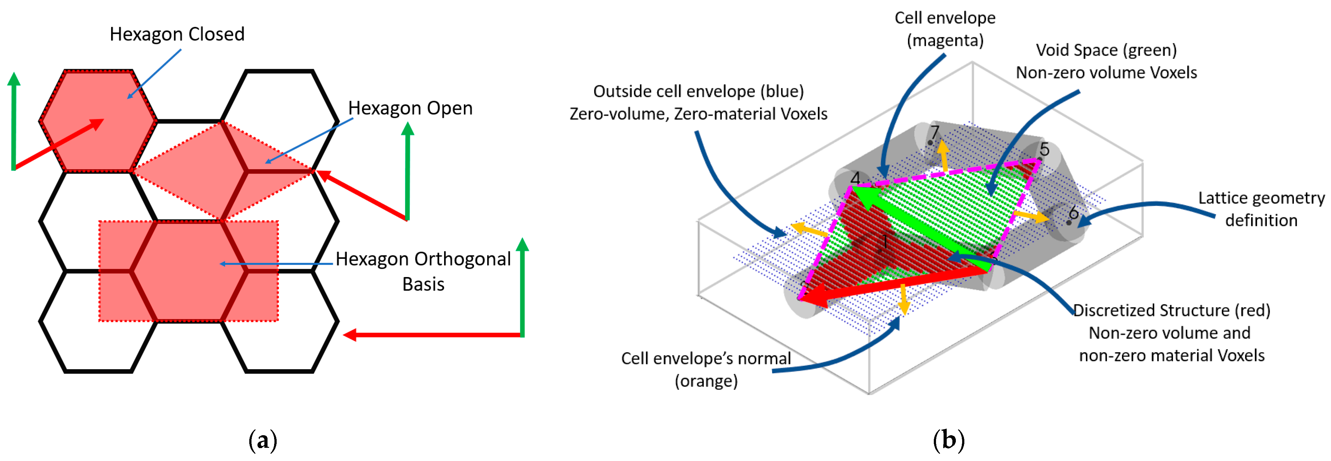
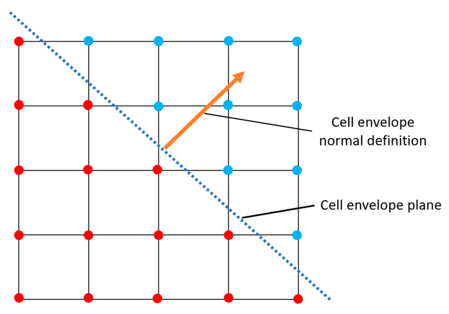
2.1. Representative Volume Element
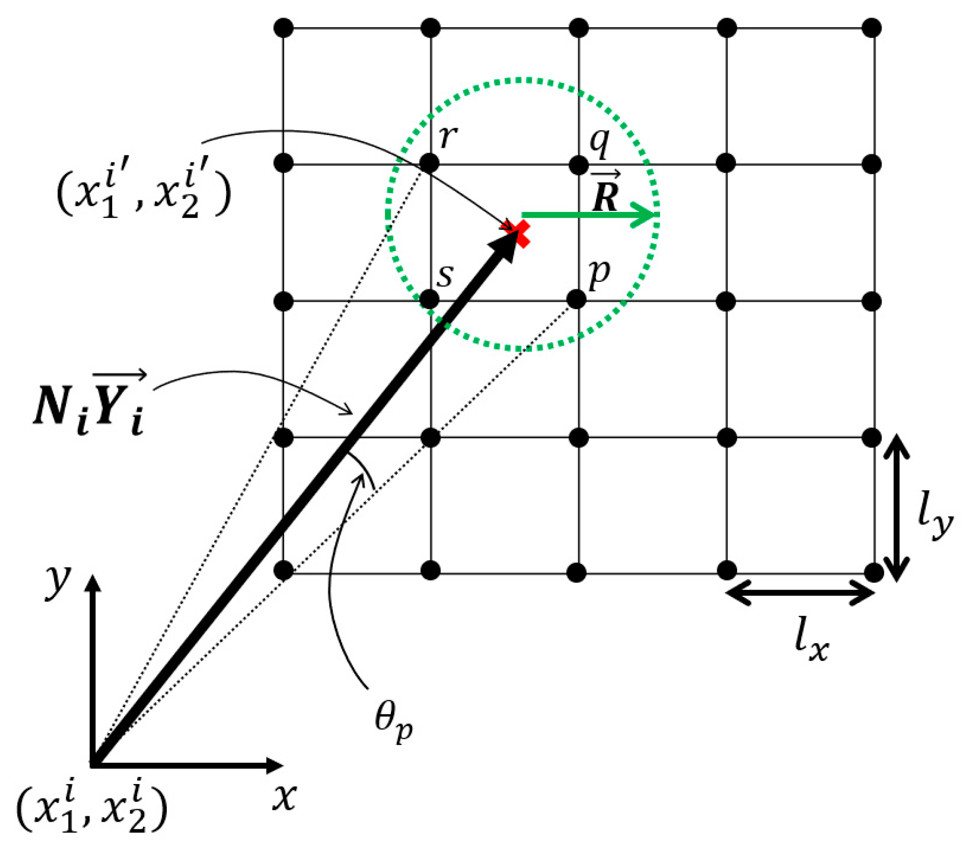
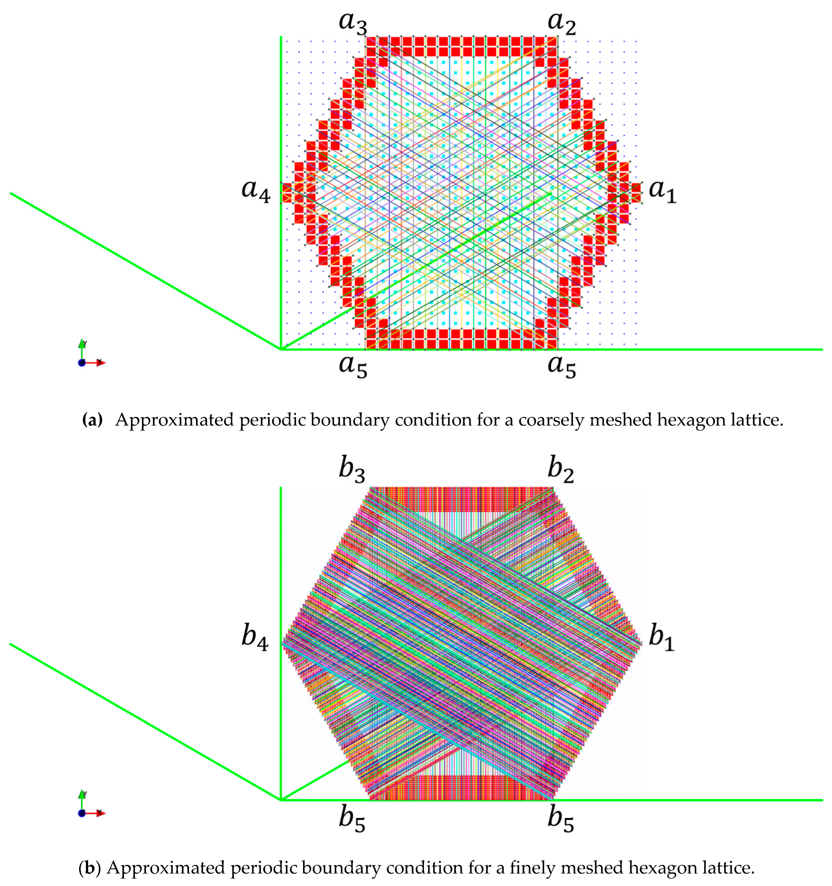
2.2. Discretization and Approximation of the Periodic Boundary Condition
2.3. Numerical Homogenization
3. Validation
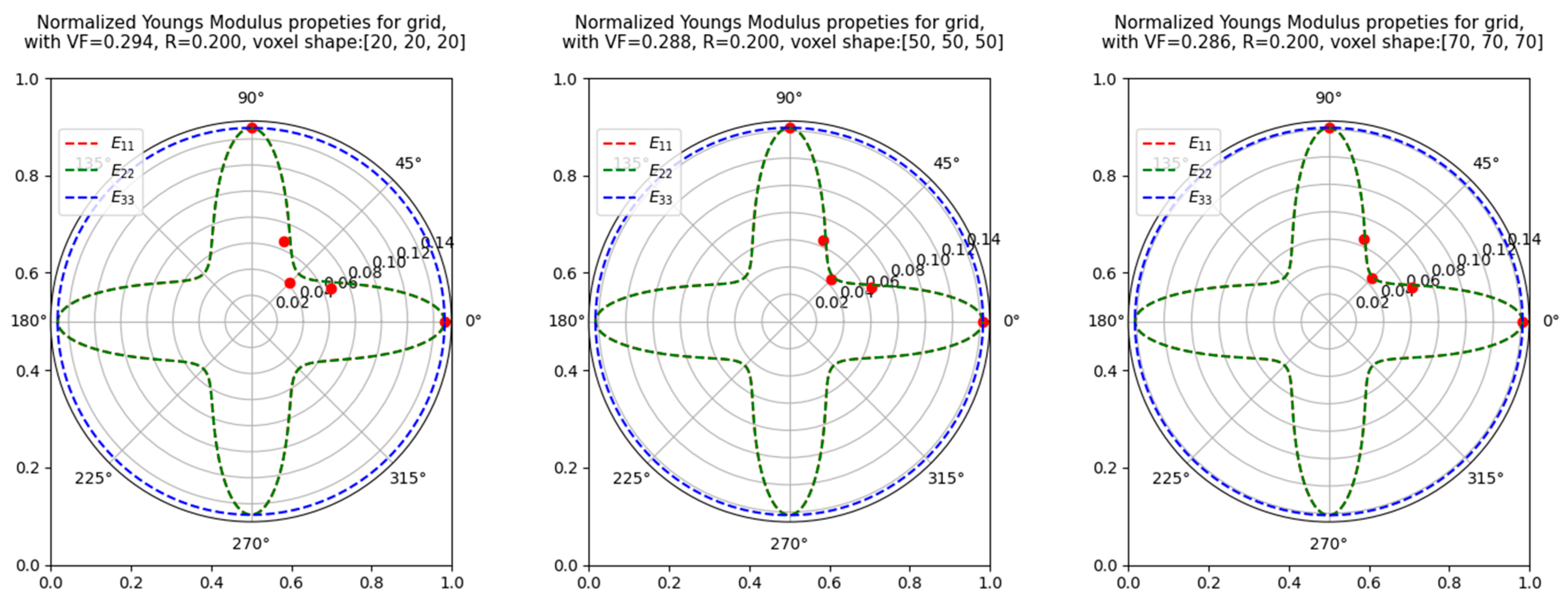
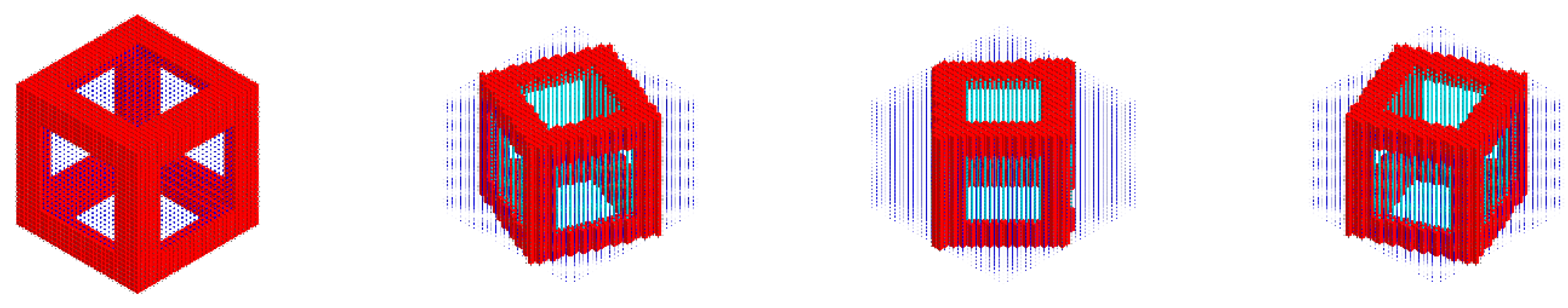
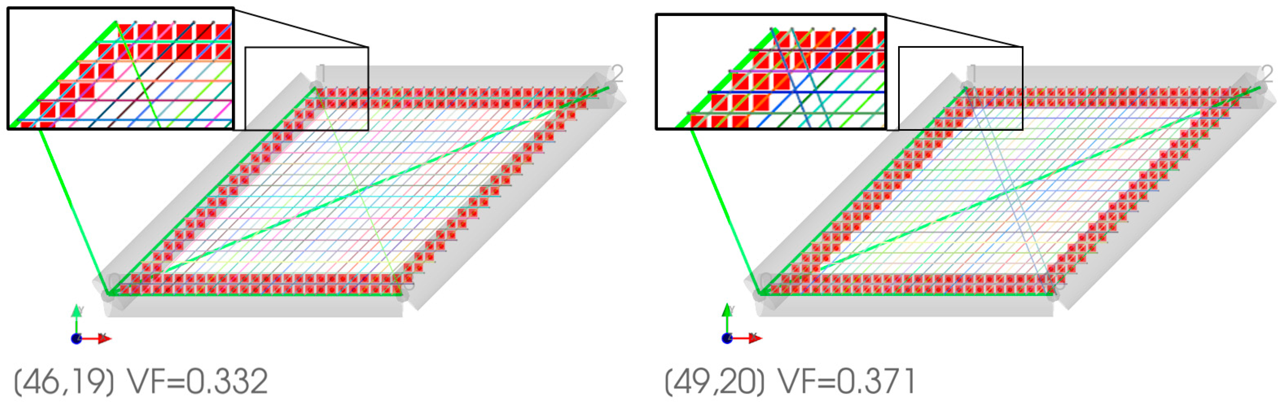
3.1. Grid Convergence Study
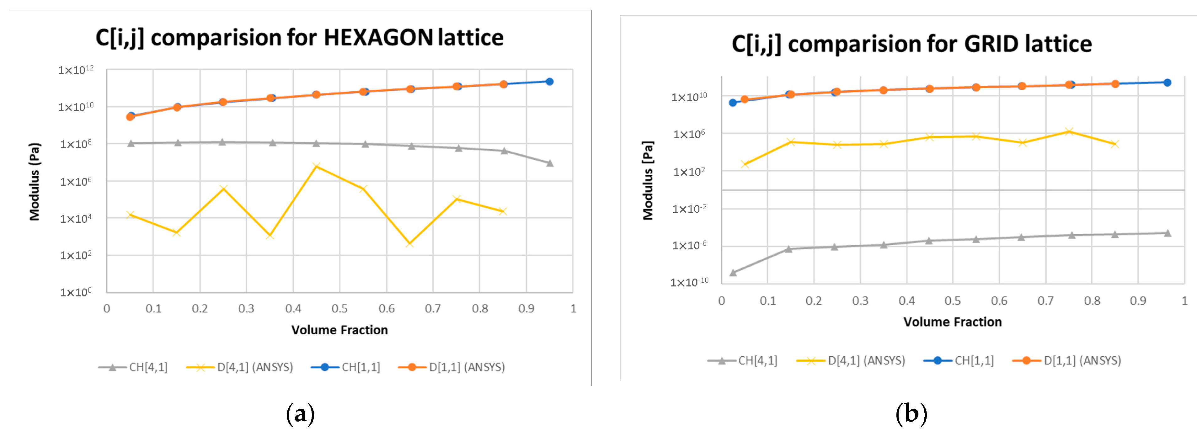
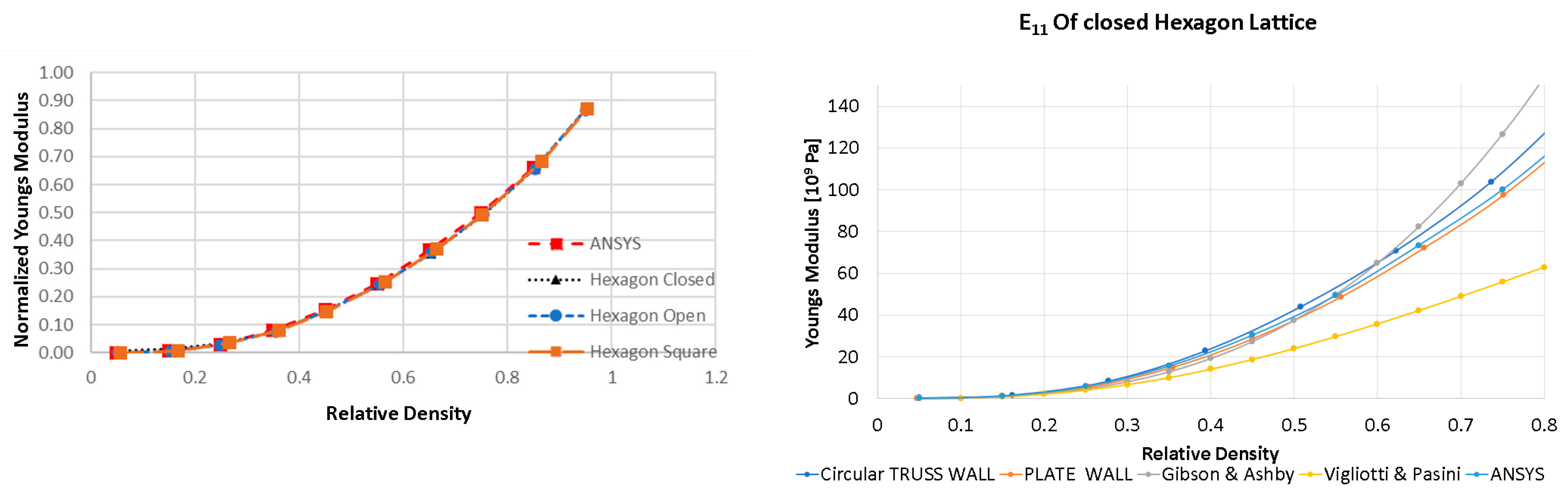
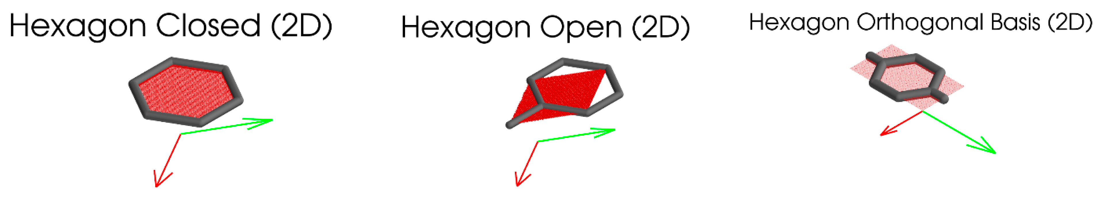
3.2. Comparison with ANSYS
3.3. RVE Rotation
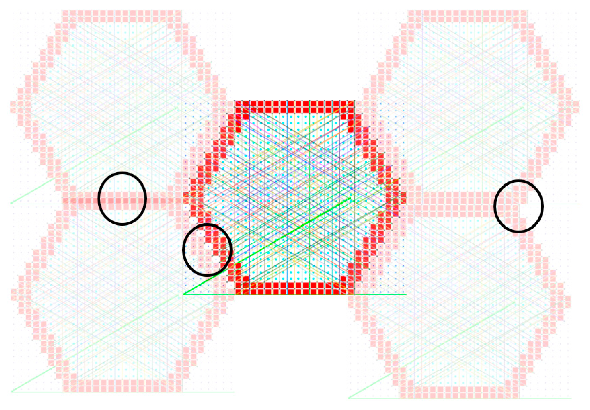
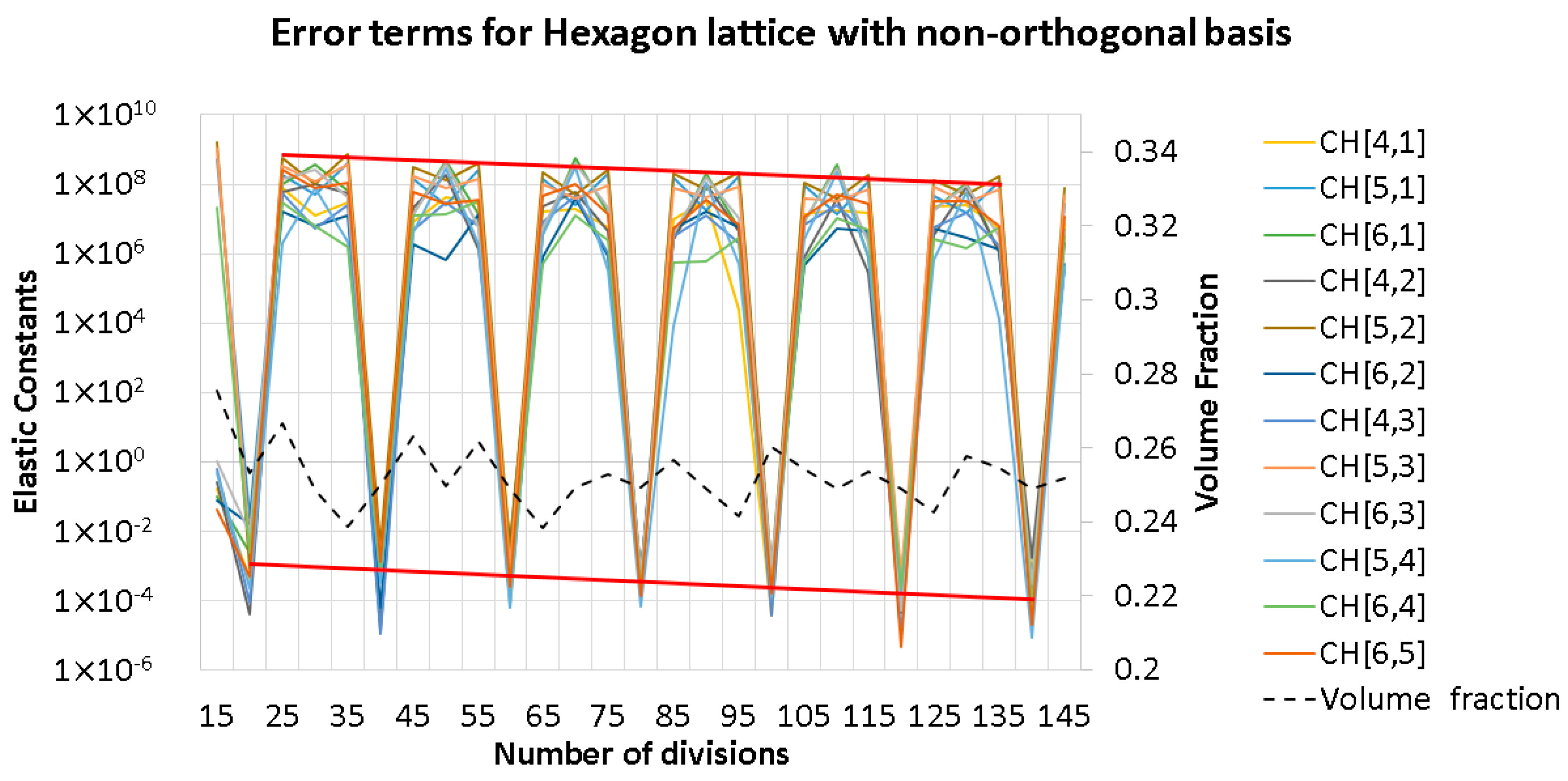
3.4. Numerical Errors Due to Approximating Periodicity
3.5. Comparison of Young’s Modulus with Volume Fraction
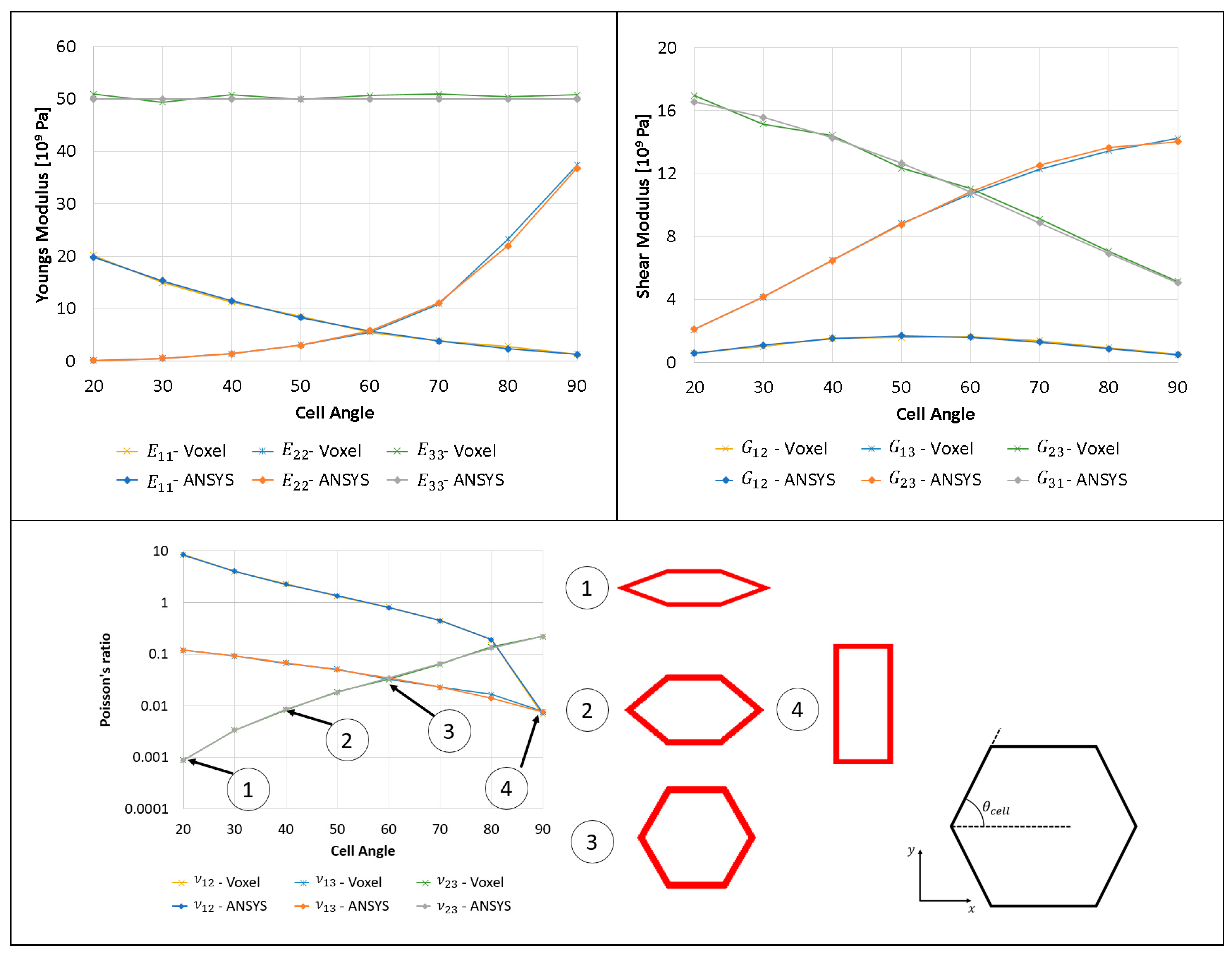
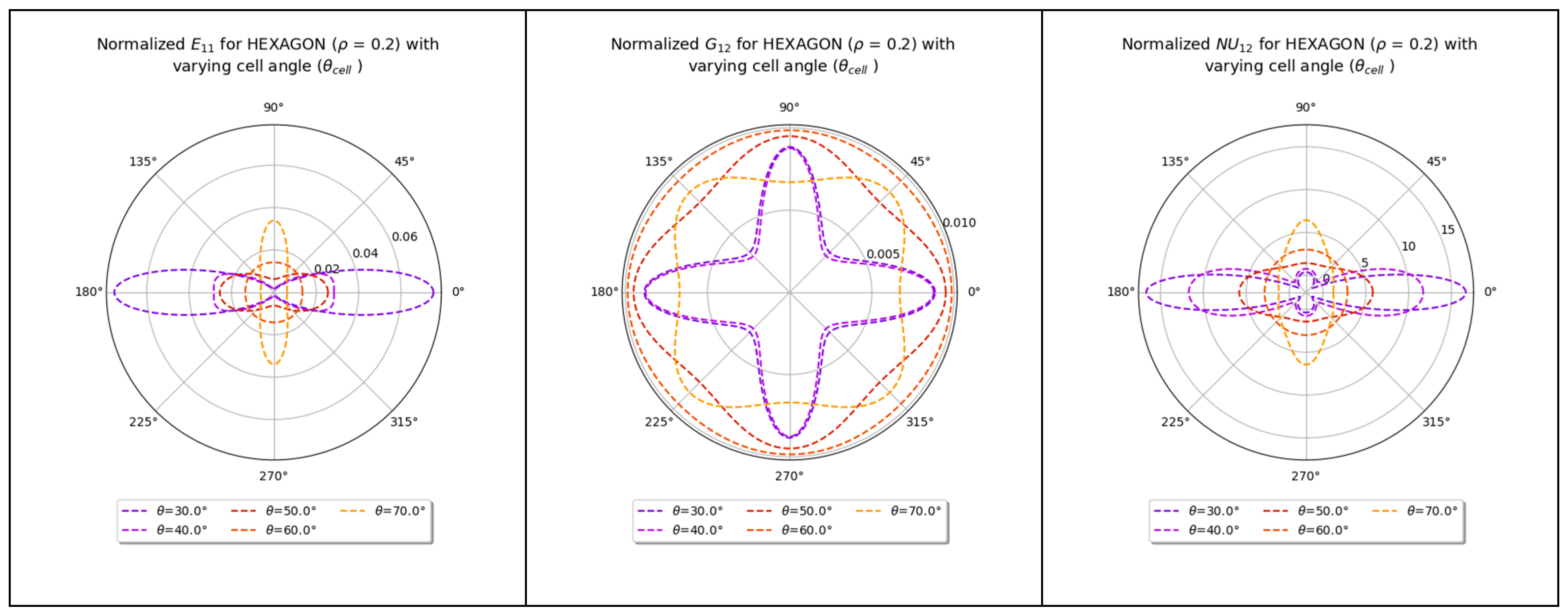
3.6. Comparison of Elastic Properties for Hexagon Lattice with Varying Cell Angle
3.7. Comparison of Elastic Constants for a 2D Monoclinic RVE Lattice with Varying Cell Angle
4. Application
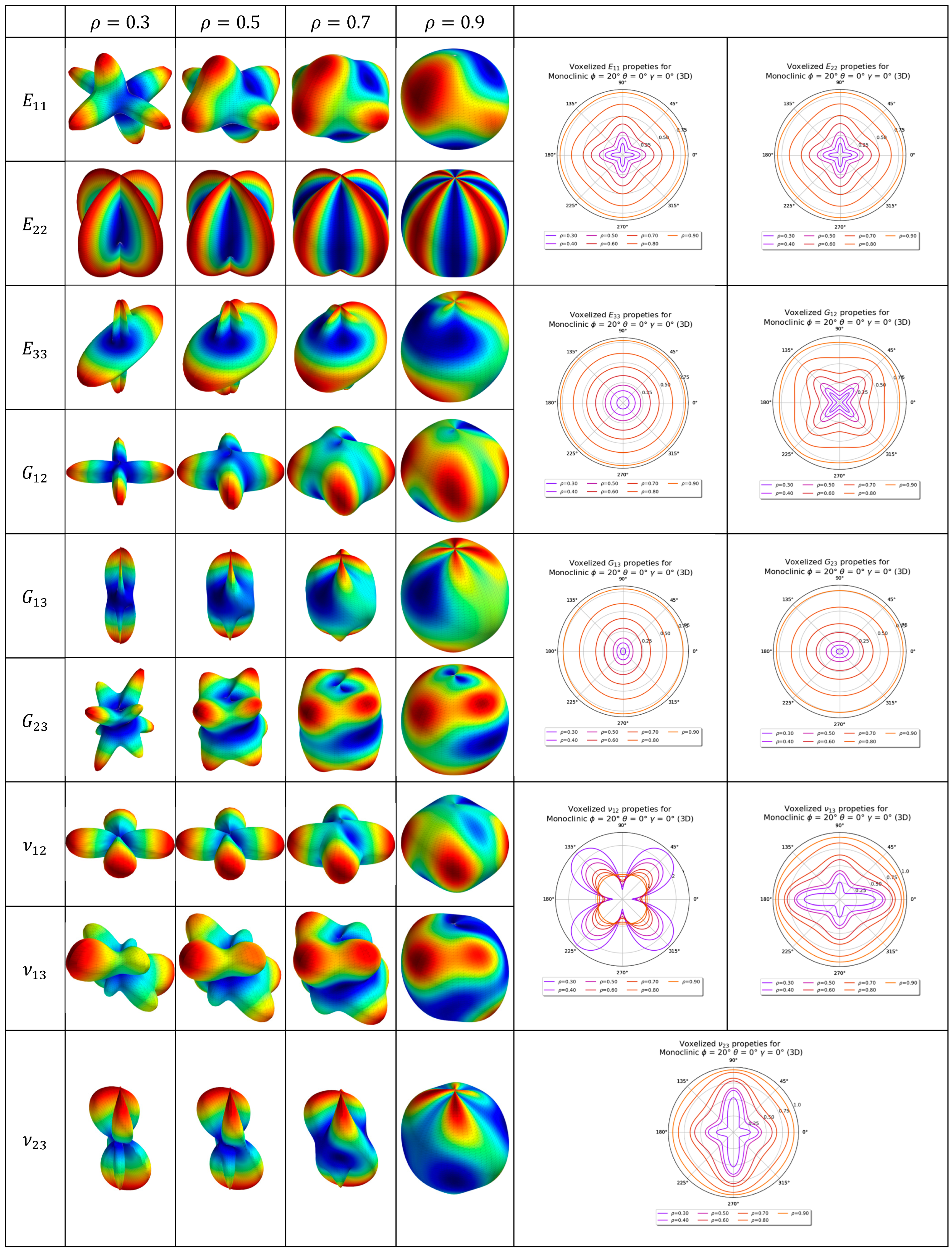
4.1. Three-Dimensional Triclinic and a Monoclinic Bravais Grid Lattice
4.2. Two-Dimensional Non-Orthogonal Lattice
4.3. Three-Dimensional Sandwich Panel Lattice
5. Conclusions
Supplementary Materials
Author Contributions
Funding
Institutional Review Board Statement
Informed Consent Statement
Data Availability Statement
Acknowledgments
Conflicts of Interest
References
- Tancogne-Dejean, T.; Spierings, A.B.; Mohr, D. Additively-Manufactured Metallic Micro-Lattice Materials for High Specific Energy Absorption under Static and Dynamic Loading. Acta Mater. 2016, 116, 14–28. [Google Scholar] [CrossRef]
- Ling, B.; Wei, K.; Wang, Z.; Yang, X.; Qu, Z.; Fang, D. Experimentally Program Large Magnitude of Poisson’s Ratio in Additively Manufactured Mechanical Metamaterials. Int. J. Mech. Sci. 2020, 173, 105466. [Google Scholar] [CrossRef]
- Wang, C.; Gu, X.; Zhu, J.; Zhou, H.; Li, S.; Zhang, W. Concurrent Design of Hierarchical Structures with Three-Dimensional Parameterized Lattice Microstructures for Additive Manufacturing. Struct. Multidiscip. Optim. 2020, 61, 869–894. [Google Scholar] [CrossRef]
- Chen, L.-Y.; Liang, S.-X.; Liu, Y.; Zhang, L.-C. Additive Manufacturing of Metallic Lattice Structures: Unconstrained Design, Accurate Fabrication, Fascinated Performances, and Challenges. Mater. Sci. Eng. R Rep. 2021, 146, 100648. [Google Scholar] [CrossRef]
- Chen, Y.; Zhao, B.; Liu, X.; Hu, G. Highly Anisotropic Hexagonal Lattice Material for Low Frequency Water Sound Insulation. Extrem. Mech. Lett. 2020, 40, 100916. [Google Scholar] [CrossRef]
- Yin, S.; Wu, L.; Yang, J.; Ma, L.; Nutt, S. Damping and Low-Velocity Impact Behavior of Filled Composite Pyramidal Lattice Structures. J. Compos. Mater. 2014, 48, 1789–1800. [Google Scholar] [CrossRef]
- Murray, G.; Gandhi, F.; Hayden, E. Polymer-Filled Honeycombs to Achieve a Structural Material with Appreciable Damping. J. Intell. Mater. Syst. Struct. 2012, 23, 703–718. [Google Scholar] [CrossRef]
- Yang, R.; Yang, Q.; Niu, B. Design and Study on the Tailorable Directional Thermal Expansion of Dual-Material Planar Metamaterial. Proc. Inst. Mech. Eng. Part C J. Mech. Eng. Sci. 2020, 234, 837–846. [Google Scholar] [CrossRef]
- Xu, H.; Farag, A.; Pasini, D. Routes to Program Thermal Expansion in Three-Dimensional Lattice Metamaterials Built from Tetrahedral Building Blocks. J. Mech. Phys. Solids J. Homepage 2018, 117, 54–87. [Google Scholar] [CrossRef]
- Wei, K.; Chen, H.; Pei, Y.; Fang, D. Planar Lattices with Tailorable Coefficient of Thermal Expansion and High Stiffness Based on Dual-Material Triangle Unit. J. Mech. Phys. Solids 2016, 86, 173–191. [Google Scholar] [CrossRef]
- Nelissen, W.E.D.; Ayas, C.; Tekõ Glu, C. 2D Lattice Material Architectures for Actuation. J. Mech. Phys. Solids J. Homepage 2019, 124, 83–101. [Google Scholar] [CrossRef]
- McHale, C.; Telford, R.; Weaver, P.M. Morphing Lattice Boom for Space Applications. Compos. Part B Eng. 2020, 202, 108441. [Google Scholar] [CrossRef]
- Li, M.Z.; Stephani, G.; Kang, K.J. New Cellular Metals with Enhanced Energy Absorption: Wire-Woven Bulk Kagome (WBK)-Metal Hollow Sphere (MHS) Hybrids. Adv. Eng. Mater. 2011, 13, 33–37. [Google Scholar] [CrossRef]
- Murray, G.J.; Gandhi, F. Auxetic Honeycombs with Lossy Polymeric Infills for High Damping Structural Materials. J. Intell. Mater. Syst. Struct. 2013, 24, 1090–1104. [Google Scholar] [CrossRef]
- Tao, Y.; Duan, S.; Wen, W.; Pei, Y.; Fang, D. Enhanced Out-of-Plane Crushing Strength and Energy Absorption of in-Plane Graded Honeycombs. Compos. Part B Eng. 2017, 118, 33–40. [Google Scholar] [CrossRef]
- Dinovitzer, M.; Miller, C.; Hacker, A.; Wong, G.; Annen, Z.; Rajakareyar, P.; Mulvihill, J.; El Sayed, M. Structural Development and Multiscale Design Optimization of Additively Manufactured UAV with Blended Wing Body Configuration Employing Lattice Materials. In Proceedings of the AIAA Scitech 2019 Forum, San Diego, CA, USA, 7–11 January 2019; American Institute of Aeronautics and Astronautics: Reston, VA, USA, 2019. [Google Scholar]
- Zhu, J.H.; Zhang, W.H.; Xia, L. Topology Optimization in Aircraft and Aerospace Structures Design. Arch. Comput. Methods Eng. 2016, 23, 595–622. [Google Scholar] [CrossRef]
- Askar, A.; Cakmak, A.S.S. A Structural Model of a Micropolar Continuum. Int. J. Eng. Sci. 1968, 6, 583–589. [Google Scholar] [CrossRef]
- Chen, J.Y.; Huang, Y.; Ortiz, M. Fracture Analysis of Cellular Materials: A Strain Gradient Model. J. Mech. Phys. Solids 1998, 46, 789–828. [Google Scholar] [CrossRef]
- Bažant, Z.P.; Christensen, M. Analogy between Micropolar Continuum and Grid Frameworks under Initial Stress. Int. J. Solids Struct. 1972, 8, 327–346. [Google Scholar] [CrossRef]
- Kumar, R.S.; McDowell, D.L. Generalized Continuum Modeling of 2-D Periodic Cellular Solids. Int. J. Solids Struct. 2004, 41, 7399–7422. [Google Scholar] [CrossRef]
- van Tuijl, R.A.; Remmers, J.J.C.; Geers, M.G.D. Multi-Dimensional Wavelet Reduction for the Homogenisation of Microstructures. Comput. Methods Appl. Mech. Eng. 2019, 359, 112652. [Google Scholar] [CrossRef]
- Vigliotti, A.; Pasini, D. Mechanical Properties of Hierarchical Lattices. Mech. Mater. 2013, 62, 32–43. [Google Scholar] [CrossRef]
- Hutchinson, R.G.; Fleck, N.A. The Structural Performance of the Periodic Truss. J. Mech. Phys. Solids 2006, 54, 756–782. [Google Scholar] [CrossRef]
- Elsayed, M.S.A.; Pasini, D. Analysis of the Elastostatic Specific Stiffness of 2D Stretching-Dominated Lattice Materials. Mech. Mater. 2010, 42, 709–725. [Google Scholar] [CrossRef]
- Vigliotti, A.; Pasini, D. Linear Multiscale Analysis and Finite Element Validation of Stretching and Bending Dominated Lattice Materials. Mech. Mater. 2012, 46, 57–68. [Google Scholar] [CrossRef]
- Florence, C.; Sab, K. A Rigorous Homogenization Method for the Determination of the Overall Ultimate Strength of Periodic Discrete Media and an Application to General Hexagonal Lattices of Beams. Eur. J. Mech. A/Solids 2006, 25, 72–97. [Google Scholar] [CrossRef]
- Assidi, M.; Dos Reis, F.; Ganghoffer, J.-F. Equivalent Mechanical Properties of Biological Membranes from Lattice Homogenization. J. Mech. Behav. Biomed. Mater. 2011, 4, 1833–1845. [Google Scholar] [CrossRef]
- Dos Reis, F.; Ganghoffer, J.F. Equivalent Mechanical Properties of Auxetic Lattices from Discrete Homogenization. Comput. Mater. Sci. 2012, 51, 314–321. [Google Scholar] [CrossRef]
- Hassani, B.; Hinton, E. A Review of Homogenization and Topology Optimization I—Homogenization Theory for Media with Periodic Structure. Comput. Struct. 1998, 69, 707–717. [Google Scholar] [CrossRef]
- Hollister, S.J.; Kikuehi, N. A Comparison of Homogenization and Standard Mechanics Analyses for Periodic Porous Composites. Comput. Mech. 1992, 10, 73–95. [Google Scholar] [CrossRef]
- Guedes, J.J.M.J.; Kikuchi, N. Preprocessing and Postprocessing for Materials Based on the Homogenization Method with Adaptive Finite Element Methods. Comput. Methods Appl. Mech. Eng. 1990, 83, 143–198. [Google Scholar] [CrossRef]
- Andreassen, E.; Andreasen, C.S. How to Determine Composite Material Properties Using Numerical Homogenization. Comput. Mater. Sci. 2014, 83, 488–495. [Google Scholar] [CrossRef]
- Dong, G.; Tang, Y.; Zhao, Y.F. A 149 Line Homogenization Code for Three-Dimensional Cellular Materials Written in MATLAB. J. Eng. Mater. Technol. Trans. ASME 2019, 141, 011005. [Google Scholar] [CrossRef]
- Masters, I.G.; Evans, K.E. Models for the Elastic Deformation of Honeycombs. Compos. Struct. 1996, 35, 403–422. [Google Scholar] [CrossRef]
- Gibson, L.J.; Ashby, M.F.; Gibson, L.J.; Ashby, M.F. Cellular Solids: Structure and Properties; Cambridge University Press: Cambridge, UK, 1997; pp. 1–510. [Google Scholar] [CrossRef]
- Christensen, R.M. Mechanics of Cellular and Other Low-Density Materials. Int. J. Solids Struct. 2000, 37, 93–104. [Google Scholar] [CrossRef]
- Elsayed, M.S.A. Multiscale Mechanics and Structural Design of Periodic Cellular Materials; McGill University: Montreal, QC, Canada, 2010. [Google Scholar]
- Vigliotti, A.; Pasini, D. Stiffness and Strength of Tridimensional Periodic Lattices. Comput. Methods Appl. Mech. Eng. 2012, 229–232, 27–43. [Google Scholar] [CrossRef]
- Kalamkarov, A.L.; Andrianov, I.V.; Danishevs’kyy, V.V. Asymptotic Homogenization of Composite Materials and Structures. Appl. Mech. Rev. 2009, 62, 030802. [Google Scholar] [CrossRef]
- Masoumi, E.; Abad, K.; Khanoki, S.A.; Pasini, D. Fatigue Design of Lattice Materials via Computational Mechanics: Application to Lattices with Smooth Transitions in Cell Geometry. Int. J. Fatigue 2012, 47, 126–136. [Google Scholar] [CrossRef]
- Cheng, G.D.; Cai, Y.W.; Xu, L. Novel Implementation of Homogenization Method to Predict Effective Properties of Periodic Materials. Acta Mech. Sin. Xuebao 2013, 29, 550–556. [Google Scholar] [CrossRef]
- Liu, P.; Liu, A.; Peng, H.; Tian, L.; Liu, J.; Lu, L. Mechanical Property Profiles of Microstructures via Asymptotic Homogenization. Comput. Graph. 2021, 100, 106–115. [Google Scholar] [CrossRef]
- Arabnejad, S.; Pasini, D. Mechanical Properties of Lattice Materials via Asymptotic Homogenization and Comparison with Alternative Homogenization Methods. Int. J. Mech. Sci. 2013, 77, 249–262. [Google Scholar] [CrossRef]
- Peng, X.; Cao, J. A Dual Homogenization and Finite Element Approach for Material Characterization of Textile Composites. Compos. Part B Eng. 2002, 33, 45–56. [Google Scholar] [CrossRef]
- Guinovart-Daz, R.; Rodrguez-Ramos, R.; Bravo-Castillero, J.; Sabina, F.J.; Dario Santiago, R.; Martinez Rosado, R. Asymptotic Analysis of Linear Thermoelastic Properties of Fiber Composites. J. Thermoplast. Compos. Mater. 2007, 20, 389–410. [Google Scholar] [CrossRef]
- Visrolia, A.; Meo, M. Multiscale Damage Modelling of 3D Weave Composite by Asymptotic Homogenisation. Compos. Struct. 2013, 95, 105–113. [Google Scholar] [CrossRef]
- Takano, N.; Zako, M.; Kubo, F.; Kimura, K. Microstructure-Based Stress Analysis and Evaluation for Porous Ceramics by Homogenization Method with Digital Image-Based Modeling. Int. J. Solids Struct. 2003, 40, 1225–1242. [Google Scholar] [CrossRef]
- Matsui, K.; Terada, K.; Yuge, K. Two-Scale Finite Element Analysis of Heterogeneous Solids with Periodic Microstructures. Comput. Struct. 2004, 82, 593–606. [Google Scholar] [CrossRef]
- Omairey, S.L.; Dunning, P.D.; Sriramula, S. Development of an ABAQUS Plugin Tool for Periodic RVE Homogenisation. Eng. Comput. 2019, 35, 567–577. [Google Scholar] [CrossRef]
- Material Designer User’s Guide. Available online: https://ansyshelp.ansys.com/account/secured?returnurl=/Views/Secured/corp/v194/acp_md/acp_md.html (accessed on 16 December 2020).
- Barbero, E.J. Finite Element Analysis of Composite Materials Using AbaqusTM.; CRC Press: Boca Raton, FL, USA, 2013; ISBN 9781466516632. [Google Scholar]
- Hassani, B.; Hinton, E. A Review of Homogenization and Topology Opimization II—Analytical and Numerical Solution of Homogenization Equations. Comput. Struct. 1998, 69, 719–738. [Google Scholar] [CrossRef]
- Hassani, B.; Hinton, E. A Review of Homogenization and Topology Optimization III—Topology Optimization Using Optimality Criteria. Comput. Struct. 1998, 69, 739. [Google Scholar] [CrossRef]
- Rajakareyar, P. Thermo-Elastic Mechanics of Morphing Lattice Structures with Applications in Shape Optimization of BLI Engine Intakes; Carleton University: Ottawa, ON, Canada, 2023. [Google Scholar]
- Virtanen, P.; Gommers, R.; Oliphant, T.E.; Haberland, M.; Reddy, T.; Cournapeau, D.; Burovski, E.; Peterson, P.; Weckesser, W.; Bright, J.; et al. SciPy 1.0: Fundamental Algorithms for Scientific Computing in Python. Nat. Methods 2020, 17, 261–272. [Google Scholar] [CrossRef]
- Kermode, J. Lars Pastewka Matscipy/Elasticity.Py at Master LibAtoms/Matscipy. Available online: https://github.com/libAtoms/matscipy/blob/master/matscipy/elasticity.py (accessed on 11 December 2020).
- Van Der Walt, S.; Colbert, S.C.; Varoquaux, G. The NumPy Array: A Structure for Efficient Numerical Computation. Comput. Sci. Eng. 2011, 13, 22–30. [Google Scholar] [CrossRef]
- SciPy. Scipy.Spatial.CKDTree—SciPy v1.5.4 Reference Guide. Available online: https://docs.scipy.org/doc/scipy/reference/generated/scipy.spatial.cKDTree.html (accessed on 11 December 2020).
- Hunter, J.D. Matplotlib: A 2D Graphics Environment. Comput. Sci. Eng. 2007, 9, 90–95. [Google Scholar] [CrossRef]
- Ramachandran, P.; Varoquaux, G. Mayavi: 3D Visualization of Scientific Data. Comput. Sci. Eng. 2011, 13, 40–51. [Google Scholar] [CrossRef]
- Gaillac, R.; Pullumbi, P.; Coudert, F.-X. ELATE: An Open-Source Online Application for Analysis and Visualization of Elastic Tensors. J. Phys. Condens. Matter 2016, 28, 275201. [Google Scholar] [CrossRef] [PubMed]
- Hoogendoorn, E.; van Golen, K. Numpy-Indexed PyPI. Available online: https://pypi.org/project/numpy-indexed/ (accessed on 11 December 2020).
- Lam, S.K.; Pitrou, A.; Seibert, S. Numba: A LLVM-Based Python JIT Compiler. In Proceedings of the Second Workshop on the LLVM Compiler Infrastructure in HPC, New York, NY, USA, 15 November 2015; pp. 1–6. [Google Scholar]


| Eigenvalues of (19) (1011) | Eigenvalues of (19) with Zeros (1011) | % Diff. | Eigenvalues of (20) (1011) | Eigenvalues of (20) with Zeros (1011) | % Diff. | % Diff. Between (19) and (20) |
|---|---|---|---|---|---|---|
| 8.0118 | 8.0117 | 0.0002 | 8.0050 | 8.0050 | 0 | 0.08 |
| 3.3757 | 3.3757 | 0.0006 | 3.4025 | 3.4025 | 0 | −0.79 |
| 1.4785 | 1.4784 | 0.0070 | 1.4104 | 1.4104 | 0 | 4.8 |
| 1.3026 | 1.3026 | −0.0009 | 1.4020 | 1.4020 | 0 | −7.1 |
| 0.5047 | 0.5048 | −0.0241 | 0.6148 | 0.6148 | 0 | −17.94 |
| 0.3390 | 0.3390 | −0.0012 | 0.3267 | 0.3267 | 0 | 3.77 |
| ) | ) | ) | |
|---|---|---|---|
| Monoclinic | |||
| Cubic, Orthorhombic, and Tetragonal |
| Elastic Properties | Monoclinic | Triclinic |
|---|---|---|
| [Pa] | 2.96 × 10¹⁰ | 2.96 × 10¹⁰ |
| [Pa] | 2.93 × 10¹⁰ | 2.27 × 10¹⁰ |
| [Pa] | 1.46 × 10¹⁰ | 9.28 × 10⁹ |
| [Pa] | 2.67 × 10⁹ | 2.68 × 10⁹ |
| [Pa] | 2.36 × 10⁹ | 2.03 × 10⁹ |
| [Pa] | 3.21 × 10⁹ | 3.36 × 10⁹ |
| 0.108 | 0.1247 | |
| 0.156 | 0.1668 | |
| 0.076 | 0.0778 |
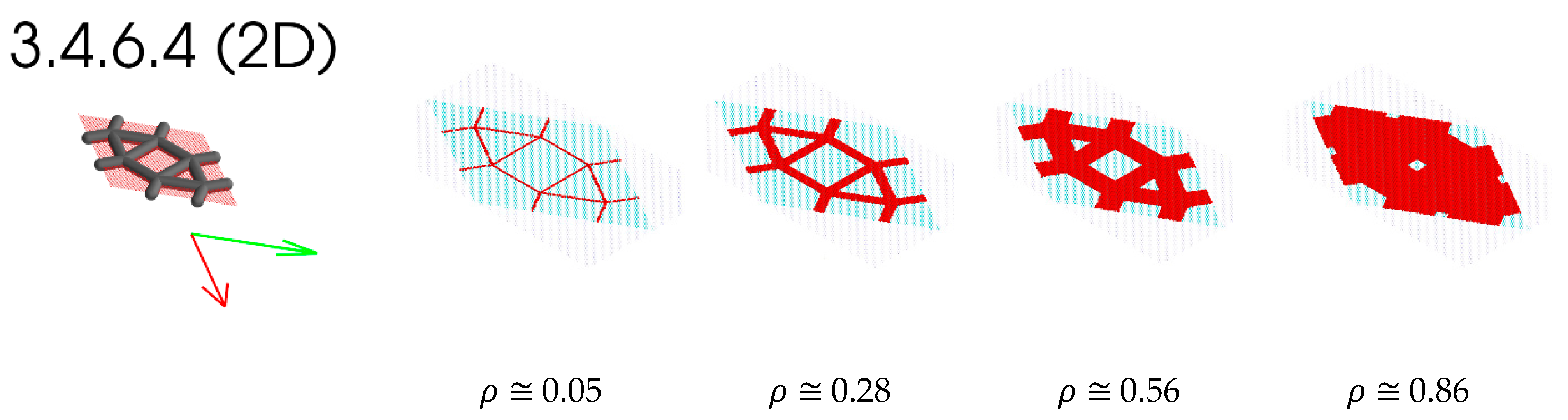
 3.4.6.4 (2D) 3.4.6.4 (2D) | 1.591 | 1.644 | 0.377 | 0.538 | 0.210 | 0.178 | 0.476 | 0.620 | 0.636 | |
| −0.662 | −0.731 | −0.189 | −0.136 | −0.014 | 0.026 | −0.351 | −0.304 | −0.325 | ||
| 0.380 | 0.390 | 1.132 | 0.011 | 0.190 | 0.180 | 0.347 | 0.218 | 0.221 | ||
| 0.999 | 0.999 | 1.000 | 1.000 | 1.000 | 1.000 | 0.995 | 0.999 | 0.999 |
 Sandwich X Lattice (3D) Sandwich X Lattice (3D) | 2.318 | 2.318 | 1.499 | 0.456 | 0.127 | 0.127 | 0.78 | 0.607 | 0.607 | |
| −1.915 | −1.915 | −0.296 | −0.387 | 0.193 | 0.193 | −0.646 | −0.265 | −0.265 | ||
| 0.941 | 0.941 | 0.118 | 0.32 | 0.045 | 0.045 | 0.365 | 0.14 | 0.14 | ||
| 0.999 | 0.999 | 1.0 | 0.999 | 0.999 | 0.999 | 0.998 | 0.995 | 0.995 |
Disclaimer/Publisher’s Note: The statements, opinions and data contained in all publications are solely those of the individual author(s) and contributor(s) and not of MDPI and/or the editor(s). MDPI and/or the editor(s) disclaim responsibility for any injury to people or property resulting from any ideas, methods, instructions or products referred to in the content. |
© 2023 by the authors. Licensee MDPI, Basel, Switzerland. This article is an open access article distributed under the terms and conditions of the Creative Commons Attribution (CC BY) license (https://creativecommons.org/licenses/by/4.0/).
Share and Cite
Rajakareyar, P.; ElSayed, M.S.A.; Abo El Ella, H.; Matida, E. Effective Mechanical Properties of Periodic Cellular Solids with Generic Bravais Lattice Symmetry via Asymptotic Homogenization. Materials 2023, 16, 7562. https://doi.org/10.3390/ma16247562
Rajakareyar P, ElSayed MSA, Abo El Ella H, Matida E. Effective Mechanical Properties of Periodic Cellular Solids with Generic Bravais Lattice Symmetry via Asymptotic Homogenization. Materials. 2023; 16(24):7562. https://doi.org/10.3390/ma16247562
Chicago/Turabian StyleRajakareyar, Padmassun, Mostafa S. A. ElSayed, Hamza Abo El Ella, and Edgar Matida. 2023. "Effective Mechanical Properties of Periodic Cellular Solids with Generic Bravais Lattice Symmetry via Asymptotic Homogenization" Materials 16, no. 24: 7562. https://doi.org/10.3390/ma16247562