Investigation of Improved Cooperative Coevolution for Large-Scale Global Optimization Problems ^†

Abstract

Modern real-valued optimization problems are complex and high-dimensional, and they are known as “large-scale global optimization (LSGO)” problems. Classic evolutionary algorithms (EAs) perform poorly on this class of problems because of the curse of dimensionality. Cooperative Coevolution (CC) is a high-performed framework for performing the decomposition of large-scale problems into smaller and easier subproblems by grouping objective variables. The efficiency of CC strongly depends on the size of groups and the grouping approach. In this study, an improved CC (iCC) approach for solving LSGO problems has been proposed and investigated. iCC changes the number of variables in subcomponents dynamically during the optimization process. The SHADE algorithm is used as a subcomponent optimizer. We have investigated the performance of iCC-SHADE and CC-SHADE on fifteen problems from the LSGO CEC’13 benchmark set provided by the IEEE Congress of Evolutionary Computation. The results of numerical experiments have shown that iCC-SHADE outperforms, on average, CC-SHADE with a fixed number of subcomponents. Also, we have compared iCC-SHADE with some state-of-the-art LSGO metaheuristics. The experimental results have shown that the proposed algorithm is competitive with other efficient metaheuristics.

1. Introduction

Evolutionary computation [1,2,3] includes a research field, where bio-inspired algorithms are used for solving global optimization problems with different levels of complexity. This family of algorithms demonstrates high performance in solving hard real-world [4,5,6,7] and benchmark [8,9] problems when the number of variables is not large (less than a hundred). In many modern real-world LSGO problems, the number of continuous variables starts from hundreds or thousands [10]. The performance of classic EAs rapidly decreases when the number of variables increases because of the curse of dimensionality [11]. Many LSGO techniques [12] use the CC approach [13] to overcome the effect of the high-dimensional search space. CC splits a vector of solution variables into the predefined number of subcomponents and optimizes them independently using an EA. CC-based metaheuristics perform well when variables are grouped correctly. The variable grouping is a challenging task for several reasons: (1) metaheuristics are limited in the number of fitness evaluations (FEVs); (2) the landscape of real-world LSGO problems is complex, (3) LSGO problems are presented by a “black-box” (BB) model.

This paper proposes a modification of the classic CC algorithm, which changes the number of variables in subcomponents dynamically during the optimization process for improving the performance of the search process. The proposed metaheuristic based on iCC uses the SHADE optimizer and is titled iCC-SHADE. iCC-SHADE performs five optimization stages. At each stage, the algorithm solves an optimization problem using 20% of the total FEVs budget. When a budget of a stage is exhausted, iCC decreases the number of subcomponents and, consequently, increases the number of variables in each subcomponent. The proposed approach efficiently implements the exploration and exploitation strategies. The exploration strategy forces an EA to discover new regions of the search space. The exploitation is performed using small subcomponents. The exploitation strategy provides an improvement of the best-found solutions. The exploration involves subcomponents of a large size, which represent an efficient problem decomposition. In [14], a survey on the balance between these two strategies is proposed.

In general, an LSGO problem can be stated as a continuous optimization problem:

$$f\left(\overline{x}\right)\to \underset{\overline{x}}{\min }$$

(1)

$$g_i\left(\overline{x}\right)\le 0,i=1,\dots ,m$$

(2)

$$h_j\left(\overline{x}\right)=0,j=1,\dots ,p$$

(3)

$$a_k\le x_k\le b_k,k=\overline{1,N},$$

(4)

where f is an objective/fitness function to be minimized, $\overline{x}$ is an N-dimensional vector of continuous variables, $f :R^N\to R^1$, $g_i$ and $h_j$ are inequality and equality constraints, respectively, $a_k$ and $b_k$ are the left and right borders of the k-th variable, respectively.

In our previous studies, we have analyzed the performance of the iCC approach when solving constrained LSGO (cLSGO) problems [15,16]. We have proposed a new benchmark set with high dimensional cLSGO problems, and have compared the performance ε-iCC-SHADE and ε-CC-SHADE algorithms. The results have demonstrated that ε-iCC-SHADE outperforms on average ε-CC-SHADE with a fixed number of subcomponents. Moreover, the results have shown that the performance of the iCC approach depends more on the decomposition of the objective than on a constraint-handling technique. In this study, we have focused on and investigated the performance of the proposed algorithms using unconstrained optimization problems only.

Based on our previous study [17], this paper has been extended with a detailed analysis of the performance of iCC-SHADE by four classes of LSGO problems, namely fully-separable, partially additively separable, overlapping, and non-separable problems. The tuned iCC-SHADE has been compared with seven state-of-the-art LSGO algorithms. The results of experiments prove the need for the fine-tuning of parameters of iCC and demonstrate an effective setting of the parameters. All numerical experiments have been confirmed by the Wilcoxon test. LSGO problems are computationally hard and expensive, thus any numerical experiments become a great challenge when using an ordinary conventional PC. We have designed a high-performance computational cluster for parallel computations, in the paper, we have provided a description on our cluster.

The paper has the following structure. Section 2 describes the main idea of CC, modern CC approaches for grouping variables, and a subcomponent optimizer in CC. The basic idea of the proposed iCC is presented in Section 3. In Section 4, we describe the experimental setup and the experimental results. Detailed information about our computational cluster is presented in Section 4.1. The study uses the LSGO CEC’13 benchmark set with 15 problems of different levels of complexity. We have compared the performance of CC-SHADE with a fixed number of subcomponents and iCC-SHADE on four different classes of LSGO problems, which are Fully-separable (Section 4.2.1), Partially Additively Separable (Section 4.2.2), Overlapping (Section 4.2.3), and Non-separable (Section 4.2.4). Section 4.2.5 demonstrates the comparison results for CC-SHADE and iCC-SHADE using all categories of benchmark problems. In Section 4.2.6, we discuss a fine-tuning of the iCC-SHADE algorithm and propose some efficient values for the number of individuals in subcomponents. In Section 4.2.7, the performance of the fine-tuned iCC-SHADE algorithm has been compared with some state-of-the-art metaheuristics. Section 5 contains conclusions and further researches.

2. Related Work

2.1. Cooperative Coevolution

CC is an effective framework for solving many hard optimization problems. When solving LSGO problems, CC is used for the decomposition of the high-dimensional problem into subcomponents that are smaller and easier for applying an EA. The original version of CC has been proposed by Potter and De Jong [18]. They have proposed two variants of CC: CCGA-1 and CCGA-2. Both algorithms decompose N-dimensional optimization problems into N 1-dimensional subcomponents. In CCGA-1, each subcomponent is optimized by its own EA using the best-found individuals from other subcomponents. CCGA-2 evolves individuals using a random collaboration of individuals from other subcomponents. The performance of CCGA-1 and CCGA-2 have been estimated using five optimization problems: Rastrigin, Schwefel, Griewangk, Ackley, and Rosenbrock. The maximum number of variables was 30. The numerical experiments have shown that CCGA-1 and CCGA-2 outperform the standard GA. GA and CCGA-2 have demonstrated equal performance and they have outperformed CCGA-1 only on the Rosenbrock problem. It can be explained by the fact that Rosenbrock has overlapped variables, and the strategy of choosing the best representative individuals in CCGA-1 leads to a stagnation of the searching process. In [18], the standard GA has been used as a subcomponent optimizer, but authors have noted that we can use any EA.

A pseudo-code of the CC framework is presented in Algorithm 1. The termination criterion is the predefined number of FEVs.

Algorithm 1. The Cooperative Coevolution framework
	Set m (the number of subcomponents), and a subcomponent optimizer (an EA)
1:	Generate an initial population;
2:	Decompose a large optimization vector into m independent subcomponents;
3:	while (termination criteria is not satisfied) do
4:	for i = 1 to m
5:	Evaluate the i-th subcomponent using the optimizer in a round-robin strategy;
6:	Construct an N-dimensional solution by merging the best-found solutions from all subcomponents;
7:	end for
8:	end while
9:	return the complete best-found solution;

2.2. LSGO Tackling Approaches

2.2.1. Non-Decomposition Methods

There are two general groups of methods for solving LSGO problems [12]: non-decomposition and CC methods. The first group optimizes the complete problem without its decomposition. Non-decomposition methods are focused mainly on creating new mutation, crossover, and selection operators, applying specialized local search algorithms, reducing the size of the population, and other techniques for enhancing the performance of the standard optimization algorithms. Some popular non-decomposition methods are IPSOLS [19], LSCBO [20], FT-DNPSO [21], GOjDE [22], LMDEa [23], C-DEEPSO [24].

2.2.2. Variable Grouping Techniques

CC approaches can be divided into three branches: static, random, and learning-based grouping techniques. Static grouping-based CC methods divide an optimization problem with N variables into the predefined number of subcomponents (m), where $N=m\times s$, and s is the number of variables in each subcomponent. If subcomponents of an LSGO problem are known, variables are grouped in subcomponents according to their type: separable and non-separable.

Random grouping CC methods assign variables in subcomponents at random after a certain number of FEV. The landscape of the optimization subproblem of each subcomponent becomes different after each random grouping. Random grouping techniques can help to avoid stagnation because a new set of variables leads to a new optimization problem. This type of methods shows good performance on some non-separable problems (with dimensionality up to one thousand). When the number of variables becomes more than 1000, the performance of random grouping techniques decreases [25].

The last group of decomposition-based methods is the learning-based dynamic grouping. The idea behind these methods is to find an interaction between variables and to group these variables into subcomponents. Usually, the interaction of variables is detected by examining each variable with others. For example, the learning-based DG approach [26] requires 1001000 FEVs if the 1000-dimensional problem is fully-separable. It is equal to 33.3% of the fitness budget for each problem from the LSGO CEC’10 [10] and CEC’13 [27] benchmarks.

Some of the popular grouping LSGO techniques are presented in Table 1. Each row in the table contains information about the authors, the year of the publication, the short name (the abbreviation) of the approach, the reference, and the type of the used grouping technique.

Table 1. LSGO grouping techniques.

Author	Year	Algorithm	Ref.	Decomposition Strategy
Potter M.A. et al.	1994	CCGA-1(2)	[18]	Static
van den Bergh F. et al.	2004	CPSO	[28]	Static
El-Abd M.	2010	CABC	[29]	Static
Shi Y. et al.	2005	CCDE	[30]	Static
Chen H. et al.	2008	CBFO	[31]	Static
Yang Z. et al.	2008	MLCC	[32]	Random
Yang Z. et al.	2008	DECC-G	[33]	Random
Li X. et al.	2012	CCPSO2	[34]	Random
Ray T. et al.	2009	CCEA-AVP	[35]	Learning
Omidvar M. N. et al.	2014	DECC-DG	[26]	Learning
Omidvar M. N. et al.	2011	CBCC-DG	[36]	Learning
Liu J. et al.	2013	CC-CMA-ES	[37]	Learning
Xiaoming X. et al.	2020	TSPDG	[38]	Learning
Lin L. et al.	2021	DGSC2	[39]	Learning
Wu X. et al.	2019	mSaDS-COA	[40]	Learning
Ren Z. et al.	2020	BHCC	[41]	Learning

2.3. Subcomponent Optimizers in Cooperative Coevolution

CC-based metaheuristics use different EAs as the subcomponent optimizer. For example, CCGA-1 and CCGA-2 use the standard genetic algorithm [18]. SaNSDE [42] (Self-adaptive differential evolution with neighborhood search) has been applied in many CC-based metaheuristics [25,33,43]. An improved version of PSO [44] has been used in [28].

In this study, the SHADE [45] (Success-History Based Parameter Adaptation for Differential Evolution) algorithm has been used as a subcomponent optimizer. SHADE is high performed differential evolution (DE) which is based on the previous modifications of DE: JADE [46], CoDE [47], EPSDE [48], and dynNP-DE [49].

SHADE uses the following features: an external archive and a historical memory. At the selection stage, replaced individuals are moved to the external archive. These individuals save information about the previous good solutions. SHADE uses them at the mutation stage for generating new individuals: $u_i=x_i+F_i·\left(x_{pbest}-x_i\right)+F_i·\left(x_{r1}-x_{r2}\right)$, where $x_i$ is the current individual, $x_{pbest}$ is a randomly selected solution from the best $\left(pop\_size·p\right)$ individuals, pop_size is the population size, p is the piece of the best individuals, $p\in \left[0;1\right]$, $F_i$ is a scale factor for the i-th individual. $r_1$ and $r_2$ are randomly selected individuals from the current population and the external archive, $r_1\in \left[1;pop\_size\right]$, $r_2\in \left[1;po{p}_{size}+\left|A\right|\right]$, here $\left|A\right|$ is the number of individuals in the external archive. The historical memory is used for recording successful values of F and CR parameters. In this study, the fine-tuned parameter values of the subcomponent optimizer (SHADE) are obtained using the grid search. According to the numerical experiments, the size of the historical memory $H$ is set to 6, the size of the external archive $arch\_size$ is set to $\left(2·po{p}_{size}\right)$, and the piece of the best individuals $p$ is set to 0.1.

3. The Proposed Approach (iCC)

One of the main parameters in the CC framework is the number of subproblems at the decomposition stage. When solving BB optimization problems, the number is not known a priori. iCC gradually increases the number of variables in subproblems. In other words, iCC reduces the total number of subproblems during the optimization process. iCC uses an equal number of FEVs for optimizing each subproblem.

Algorithm 2 shows a pseudo-code for iCCEA. We can use any EA (or another metaheuristic) as the optimizer for subproblems. In the study, iCC uses the following numbers of subproblems, $S=\left\{10, 8, 4, 2, 1\right\}$. The number of FEVs for each stage is calculated as $iCCFEVs=\frac{MAX\_FEVs}{\left|S\right|}$, where MAX_FEVs is the budget of fitness evaluations in one run, $\left|S\right|$ is the cardinality of S (the total number of stages of iCC). We have also investigated the strategy with decreasing the number of variables for each subproblem, but its performance is too low.

Algorithm 2. Pseudo-code of iCCEA
	Set EA, pop_size, $S=\left\{10, 8, 4, 2, 1\right\}$, $iCCFEVs=\frac{MAX\_FEVs}{\left|S\right|}$, iCC_index = 1, FEV_counter = 0;
1:	m = $S_{iCC\_index}$;
2:	for i = 1 to m
3:	Generate the initial population;
4:	Evaluate the i-th subcomponent using EA in a round-robin strategy;
5:	FEV_counter++;
6:	end for
7:	while (termination criteria is not satisfied) do
8:	for i=1 to $S_{iCC\_index}$
9:	Apply EA operators to the i-th subcomponent;
10:	Evaluate the fitness function for each individual in the i-th subcomponent;
11:	FEV_counter++;
12:	end for
13:	if (FEV_counter > iCCFEVs) then
14:	iCC_index++;
15:	FEV_counter = 0;
16:	end if
17:	end while
18:	returnthe best-found solution;

4. Experimental Setup and Results

This section gives information about our computational cluster and the experimental results. We have used an actual version of the LSGO benchmark set [27]. The benchmark contains fifteen hard high-dimensional optimization problems. The dimensionality for all problems is set to 1000. We use the following settings for all experiments: the number of independent runs for each problem is 25, 3.0 × 10⁶ FEVs is the budget for one independent run.

4.1. Our Computational Cluster

LSGO benchmarks and many real-world problems require a large number of computing resources, thus it is hard to make numerical experiments using a regular PC. In [27], the authors have presented the required time for evaluating the LSGO benchmark using Intel(R) Core(TM)2 Duo CPU E8500 @3.16 GHz. All our experiments using this CPU in the single-thread mode require about 258 days. Our cluster evaluates the benchmark in less than two weeks. The cluster uses C++ programming language and operates in Ubuntu 20.04 LTS. The detailed description of each computing node is presented in Table 2. Figure 1 presents the structure of our cluster. We have five PCs: one Master-PC and four Slave-PCs. Master-PC sends computational tasks to all Slave-PCs. All numerical results are collected in *.txt files and are stored in Master-PC. We use MPICH2 (Message Passing Interface Chameleon) [50] for connecting computers together and solving parallel tasks. The cluster model is scalable. The complete code of the iCC-SHADE algorithm is available at GitHub (https://github.com/VakhninAleksei/MDPI_Algorithms_2021-iCC-SHADE, accessed on 31 March 2021).

Table 2. Specification of the computational cluster.

Name of Node	CPU	Cores/Threads	Base Clock	RAM
Master-PC	Ryzen 1700x	8/16	3.4 GHz	16 Gb
Slave 1-PC	Ryzen 2700	8/16	3.2 GHz	8 Gb
Slave 2-PC	Ryzen 2700	8/16	3.2 GHz	8 Gb
Slave 3-PC	Ryzen 2700	8/16	3.2 GHz	8 Gb
Slave 4-PC	Ryzen PRO 2700	8/16	3.2 GHz	8 Gb

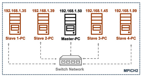
Figure 1. The structure of the computational cluster using MPICH2.

4.2. Numerical Experiments

This subsection presents the experimental results of iCC-SHADE and CC-SHADE with the fixed number of subcomponents for the LSGO CEC’13 benchmark. We have used the following settings for CC-SHADE and iCC-SHADE: the population size for each subcomponent is $pop\_size=\left\{25, 50, 100, 150, 200\right\}$, the number of subcomponents is $m=\left\{1, 2, 4, 8, 10\right\}$, $s=\left\{10, 8, 4, 2, 1\right\}$, the size of an external archive is $\left(2·pop\_size\right)$. We use “CC(m)” and “iCC” notations, where CC(m) is CC-SHADE with m fixed subcomponents, and iCC is iCC-SHADE.

4.2.1. Fully Separable Problems

We will describe features of fully separable optimization problems and how metaheuristics perform on these problems. F₁-F₃ benchmark problems belong to this class.

Definition 1.

A function$f\left(x_1,x_2,\dots ,x_N\right)$is fully separable if:$\underset{\left(x_1,x_2,\dots ,x_N\right)}{argmin}f\left(x_1,x_2,\dots ,x_N\right)=\left(\underset{x_1}{argmin}f\left(x_1,x_2,\dots ,x_N\right),\underset{x_2}{argmin}f\left(x_1,x_2,\dots ,x_N\right),\dots ,\underset{x_N}{argmin}f\left(x_1,x_2,\dots ,x_N\right)\right)$.

In other words, we can find the global optimum of a separable problem by optimizing each variable independently from other variables. An example of a fully separable problem is

$$f\left(\overline{x}\right)=x_1^2+x_2^2+x_3^2.$$

(5)

We have estimated the performance of CC(m) and iCC on the fully separable problems (F₁–F₃). Figure 2 shows the average ranks of metaheuristics with the different numbers of pop_size. Ranks are based on the mean values, which are obtained from 25 independent runs. The lowest mean value gives the highest rank.

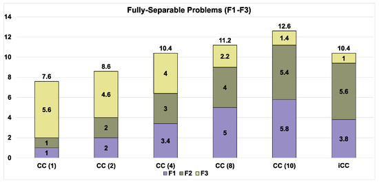
Figure 2. Average ranks of algorithms on F1–F3 problems.

As we can see from Figure 2, the performance of decomposition-based algorithms strongly depends on the number of subcomponents. We can observe this dependence on F₁ and F₂. For F₃, CC(10) demonstrates better results on average. iCC shares third place with CC(8) on all fully separable functions. CC(10) and CC(8) have taken first and second place, respectively.

Table 3 shows the statistical difference in the results. We use the Wilcoxon rank-sum test (p-value equals to 0.01) to prove the difference. Each cell in Table 3 has the following values: “better/worse/equal”. Table 4 contains the sum of (better/worse/equal) points of all algorithms.

Table 3. The results of the Wilcoxon test for CC and iCC with different population sizes.

Number	Algorithm	(2)	(3)	(4)	(5)	(6)
(1)	CC(1)	5/9/1	5/10/0	5/10/0	5/10/0	5/10/0
(2)	CC(2)	-	5/10/0	5/10/0	5/10/0	5/10/0
(3)	CC(4)	-	-	5/10/0	5/10/0	7/7/1
(4)	CC(8)	-	-	-	5/9/1	9/6/0
(5)	CC(10)	-	-	-	-	9/0/6
(6)	iCC	-	-	-	-	-

Table 4. The sum of the Wilcoxon test results.

Number	Algorithm	Win	Loss	Equal	Av. Rank
(5)	CC(10)	48	20	7	12.6
(4)	CC(8)	45	29	1	11.2
(3)	CC(4)	37	37	1	10.4
(6)	iCC	33	35	7	10.4
(2)	CC(2)	29	45	1	8.6
(1)	CC(1)	25	49	1	7.6

Figure 3 shows convergence graphs for CC(m) and iCC. The dotted vertical lines in convergence graphs (20%, 40%, 60%, and 80% of FEVs) demonstrate generations when iCC changes the number of subcomponents. As we can see, iCC always demonstrates the same performance as CC(10) during the first 20% of FEVs, because iCC starts with 10 subcomponents.

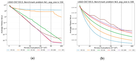
Figure 3. Convergence graphs for CC(m) and iCC on F₁, and F₃ problems with different population size (format: F_#-pop_size): (a) F₁-150; (b) F₃-100.

4.2.2. Partially Additively Separable Problems

Definition 2.

A function$f\left(x_1,x_2,\dots ,x_N\right)$is partially separable with m independent subcomponents iff:$\underset{\left(x_1,x_2,\dots ,x_N\right)}{argmin}f\left(x_1,x_2,\dots ,x_N\right)=\left(\underset{x_1}{argmin}f\left(x_1,\dots \right),\dots ,\underset{x_m}{argmin}f\left(\dots ,x_m\right)\right)$, where$x_1,\dots ,x_m$are disjoint sub-vectors of$\left(x_1,x_2,\dots ,x_N\right)$and$2\le m\le N$.

An example of a partially separable problem with 2 independent subcomponents is

$$f\left(\overline{x}\right)=x_1^2{x}_2^2+x_3^2.$$

(6)

Partially Additively Separable Problems in the benchmark are F₄–F₁₁. The average ranks for CC(m) and iCC are presented in Figure 4. As we can see, CC(4) demonstrates the best performance in comparison with all algorithms with the fixed numbers of subcomponents. iCC demonstrates the best result in comparison with all CC(m). Table 5 and Table 6 have the same structure as Table 3 and Table 4, respectively. iCC has the maximum number of “win” and the minimum number of “loss” points in comparison with all CC(m). Figure 5 shows convergence graphs for CC(m) and iCC.

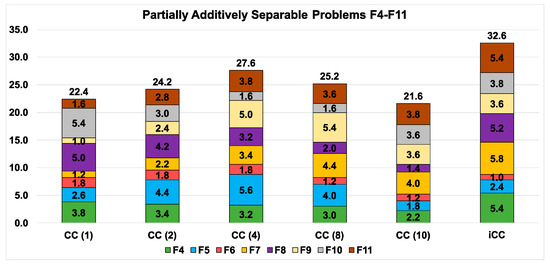
Figure 4. Average ranks of algorithms on the F₄–F₁₁ problems.

Table 5. The results of the Wilcoxon test for CC and iCC with different population sizes.

Number	Algorithm	(2)	(3)	(4)	(5)	(6)
(1)	CC(1)	6/19/15	13/21/6	17/19/4	18/16/6	14/19/7
(2)	CC(2)	-	8/14/18	13/14/13	17/11/12	9/20/11
(3)	CC(4)	-	-	10/8/22	18/9/13	12/17/11
(4)	CC(8)	-	-	-	9/2/29	6/13/21
(5)	CC(10)	-	-	-	-	1/15/24
(6)	iCC	-	-	-	-	-

Table 6. The sum of the Wilcoxon test results.

Number	Algorithm	Win	Loss	Equal	Av. Rank
(6)	iCC	84	42	74	32.6
(3)	CC(4)	75	55	70	27.6
(4)	CC(8)	56	55	89	25.2
(2)	CC(2)	66	65	69	24.2
(1)	CC(1)	68	94	38	22.4
(5)	CC(10)	39	77	84	21.6

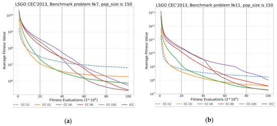
Figure 5. Convergence graphs for CC(m) and iCC on F₇, and F₁₁ problems with different population size (F_#-pop_size: (a) F₇-150; (b) F₁₁-150).

4.2.3. Overlapping Problems

Definition 3.

A function$f\left(x_1,x_2,\dots ,x_N\right)$ is overlapping if the subcomponents of these functions have some degree of overlap with its neighboring subcomponents.

An example of an optimization problem with overlapping variables is

$$f\left(\overline{x}\right)=x_1{x}_2+x_2{x}_3,$$

(7)

where $x_2$ belongs to both subcomponents $x_1{x}_2$ and $x_2{x}_3$.

F₁₂–F₁₄ are problems from the overlapping class. The experimental results are shown in Figure 6 and Figure 7, and Table 7 and Table 8. Table 7 and Table 8 have the same structure as Table 3 and Table 4, respectively. We can see that iCC outperforms all CC(m) algorithms. iCC has the maximum and the minimum number of “win” and “loss” points, respectively, in comparison with CC(m) algorithms.

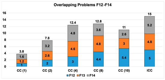
Figure 6. Average ranks of algorithms on the F₁₂–F₁₄ problems.

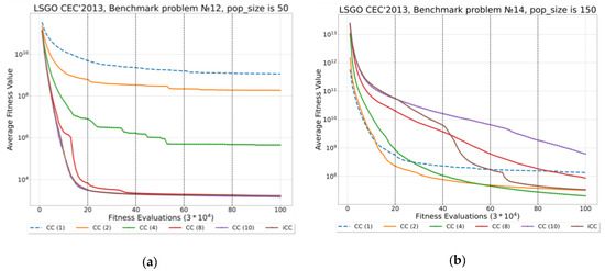
Figure 7. Convergence graphs for CC(m) and iCC on F₁₂ and F₁₄ with different population size (F_#-pop_size: (a) F₁₂-25; (b) F₁₄-150).

Table 7. The results of the Wilcoxon test for CC and iCC with different population sizes.

Number	Algorithm	(2)	(3)	(4)	(5)	(6)
(1)	CC(1)	0/12/3	0/15/0	0/14/1	1/12/2	0/15/0
(2)	CC(2)	-	0/13/2	3/10/2	4/10/1	1/10/4
(3)	CC(4)	-	-	4/8/3	5/7/3	4/9/2
(4)	CC(8)	-	-	-	6/3/6	0/5/10
(5)	CC(10)	-	-	-	-	1/5/9
(6)	iCC	-	-	-	-	-

Table 8. The sum of the Wilcoxon test results.

Number	Algorithm	Win	Loss	Equal	Av. Rank
(6)	iCC	44	6	25	15
(4)	CC(8)	38	15	22	12.8
(3)	CC(4)	41	24	10	12.4
(5)	CC(10)	33	21	21	11
(2)	CC(2)	20	43	12	7.8
(1)	CC(1)	1	68	0	3.8

4.2.4. Non-Separable Problems

Definition 4.

A function$f\left(x_1,x_2,\dots ,x_N\right)$ is fully-nonseparable if every pair of its decision variables interact with each other.

An example of a fully-nonseparable optimization problem is

$$f\left(\overline{x}\right)=x_1^2{x}_2^2{x}_3.$$

(8)

F₁₅ is the only problem of this class in the LSGO CEC’13 benchmark. The experimental results are shown in Figure 8 and Figure 9, and Table 9 and Table 10. The CC(10) algorithm demonstrates the best results in comparison with all CC(m) and iCC. As we can see, iCC has taken third place in comparison with CC(m).

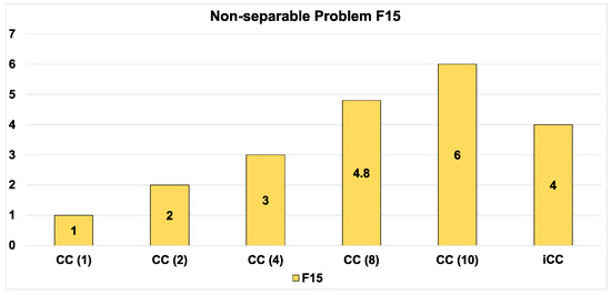
Figure 8. Average ranks of algorithms on the F₁₅ problem.

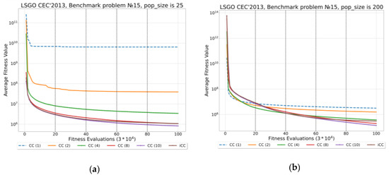
Figure 9. Convergence graphs for CC(m) and iCC on F₁₅ with different population size (F_#-pop_size: (a) F₁₅-25; (b) F₁₅-200).

Table 9. The results of the Wilcoxon test for CC and iCC with different population sizes.

Number	Algorithm	(2)	(3)	(4)	(5)	(6)
(1)	CC(1)	0/5/0	0/5/0	0/5/0	0/5/0	0/5/0
(2)	CC(2)	-	0/5/0	0/5/0	0/5/0	0/5/0
(3)	CC(4)	-	-	0/5/0	0/5/0	0/5/0
(4)	CC(8)	-	-	-	0/5/0	4/0/1
(5)	CC(10)	-	-	-	-	5/0/0
(6)	iCC	-	-	-	-	-

Table 10. The sum of the Wilcoxon test results.

Number	Algorithm	Win	Loss	Equal	Av. Rank
(5)	CC(10)	25	0	0	6
(4)	CC(8)	4	20	1	4.8
(6)	iCC	15	9	1	4
(3)	CC(4)	10	15	0	3
(2)	CC(2)	5	20	0	2
(1)	CC(1)	0	25	0	1

4.2.5. Comparison of CC vs. iCC on the Whole LSGO Benchmark

We have compared the performance of CC(m) and iCC on all four classes of LSGO problems. We use the following notation: C1 for “Fully Separable Problems”, C2 for “Partially Additively Separable Problems”, C3 for “Overlapping Problems”, and C4 for “Non-separable Problems”. The full comparison is presented in Figure 10, Table 11 and Table 12. iCC has got the highest rank in comparison with CC(m). iCC has the biggest and the lower numbers of “win” and “lose” points, respectively. Figure 11 shows convergence graphs for iCC with different population sizes on F₄ and F₁₄, problems.

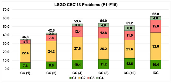
Figure 10. Average ranks of algorithms on the F₁–F₁₅ problems.

Table 11. The results of the Wilcoxon test for CC and iCC with different population sizes.

Number	Algorithm	(2)	(3)	(4)	(5)	(6)
(1)	CC(1)	11/45/19	18/51/6	22/48/5	24/43/8	19/49/7
(2)	CC(2)	-	13/42/20	21/39/15	26/36/13	15/45/15
(3)	CC(4)	-	-	19/31/25	28/31/16	23/38/14
(4)	CC(8)	-	-	-	20/19/36	19/24/32
(5)	CC(10)	-	-	-	-	16/20/39
(6)	iCC	-	-	-	-	-

Table 12. The sum of the Wilcoxon test results.

Number	Algorithm	Win	Loss	Equal	Av. Rank
(6)	iCC	176	92	107	62
(4)	CC(8)	157	105	113	54
(3)	CC(4)	163	131	81	53.4
(5)	CC(10)	145	118	112	51.2
(2)	CC(2)	120	173	82	42.6
(1)	CC(1)	94	236	45	34.8

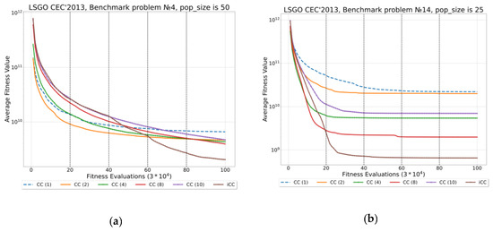
Figure 11. Convergence graphs for CC and iCC on F₄ and F₁₄ with different population size (F_#-pop_size: (a) F₄-50; (b) F₁₄-25)

4.2.6. Tuning iCC

We have investigated the effect of fine-tuning for iCC. iCC has only one control parameter, that is the population size. We have compared iCC with different population sizes: 25, 50, 100, 150, and 200. The experimental results are presented in Figure 12 as average ranks of algorithms. iCC with 150 individuals outperforms other variants of iCC. Table 13 and Table 14 prove experimental results using Wilcoxon test. Figure 13 shows convergence graphs for iCC with different population sizes on F₁ and F₇, problems.

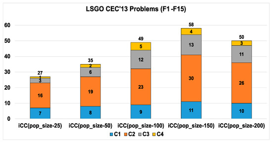
Figure 12. Average ranks of algorithms, when tuning the population size of iCC algorithms.

Table 13. The results of the Wilcoxon test for iCC with different population sizes.

Number	Algorithm	(2)	(3)	(4)	(5)
(1)	iCC(pop_size-25)	2/11/2	3/11/1	3/11/1	3/11/1
(2)	iCC(pop_size-50)	-	3/10/2	2/11/2	3/9/3
(3)	iCC(pop_size-100)	-	-	1/3/11	2/2/11
(4)	iCC(pop_size-150)	-	-	-	3/2/10
(5)	iCC(pop_size-200)	-	-	-	-

Table 14. The sum of the Wilcoxon test results.

Number	Algorithm	Win	Loss	Equal	Av. Rank
(4)	iCC(pop_size-150)	28	8	24	58
(5)	iCC(pop_size-200)	24	11	25	50
(3)	iCC(pop_size-100)	24	11	25	49
(2)	iCC(pop_size-50)	19	32	9	35
(1)	iCC(pop_size-25)	11	44	5	27

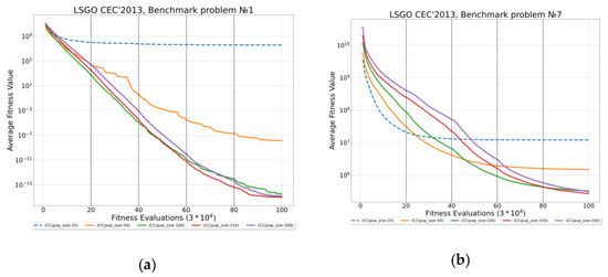
Figure 13. Convergence graphs for iCC on F₁ (a), and F₇ (b) with different population size.

4.2.7. Comparison with Some State-of-The-Art Metaheuristics

We have compared fine-tuned iCC-SHADE with the following metaheuristics: SHADEILS [51], CC-RDG3 [52], IHDELS [53], SACC [54], MPS [55], VMODE [56], and SGCC [57]. These state-of-the-art metaheuristics were specially created for solving LSGO problems. We have used the Formula-1 scoring system for ranking the mean best-found values. The list of points is the following: “25, 18, 15, 12, 10, 8, 6, 4, 2, 1”. As we compare eight metaheuristics, the best-performed and the worst-performed algorithm will get 25 and 4 points, respectively.

Table 15 shows the experimental results Each cell contains the value averaged over 25 independent runs. Table 16 and Figure 14 are based on Table 15 results and the Formula-1 scoring system. In Table 16, the first row denotes the algorithms, the first column denotes classes of functions that are described in Section 4.2.5. Fine-tuned iCC-SHADE has taken fourth place. iCC-SHADE does not dominate in some classes.

Table 15. iCC-SHADE vs. state-of-the-art metaheuristic.

#	SHADEILS	CC-RDG3	IHDELS	iCC-SHADE	SACC	MPS	VMODE	SGCC
1	2.69 × 10−24	1.14 × 10−18	4.80 × 10−29	1.01 × 10−17	0.00	6.68 × 108	8.51 × 10−4	1.85 × 103
2	1.00 × 103	2.31 × 103	1.27 × 103	9.37 × 102	5.71 × 102	4.20 × 103	5.51 × 103	8.94 × 103
3	2.01 × 10	2.04 × 10	2.00 × 10	2.07 × 10	1.21	1.94	3.41 × 10−4	2.15 × 10
4	1.48 × 108	4.29 × 104	3.09 × 108	9.71 × 108	3.66 × 1010	1.07 × 1011	8.48 × 109	1.23 × 109
5	1.39 × 106	2.04 × 106	9.68 × 106	2.47 × 106	6.95 × 106	1.20 × 106	7.28 × 1014	5.02 × 106
6	1.02 × 106	1.00 × 106	1.03 × 106	1.06 × 106	2.07 × 105	6.01 × 103	1.99 × 105	1.06 × 106
7	7.41 × 10	1.71 × 10−21	3.18 × 104	2.70 × 105	1.58 × 107	7.19 × 107	3.44 × 106	1.83 × 105
8	3.17 × 1011	7.11 × 103	1.36 × 1012	2.84 × 1012	9.86 × 1014	2.04 × 1014	3.26 × 1013	1.54 × 1011
9	1.64 × 108	1.57 × 108	7.12 × 108	1.66 × 108	5.77 × 108	1.66 × 108	7.51 × 108	4.06 × 108
10	9.18 × 107	9.16 × 107	9.19 × 107	9.32 × 107	2.11 × 107	3.53 × 106	9.91 × 106	9.38 × 107
11	5.11 × 105	2.18 × 10−13	9.87 × 106	1.94 × 107	5.30 × 108	2.20 × 109	1.58 × 108	2.55 × 107
12	6.18 × 10	7.00 × 102	5.16 × 102	1.14 × 103	8.74 × 102	1.75 × 104	2.34 × 103	3.56 × 103
13	1.00 × 105	6.43 × 104	4.02 × 106	1.41 × 107	1.51 × 109	9.87 × 108	2.43 × 107	1.21 × 107
14	5.76 × 106	1.65 × 109	1.48 × 107	3.38 × 107	7.34 × 109	1.03 × 109	9.35 × 107	2.07 × 107
15	6.25 × 105	2.30 × 106	3.13 × 106	2.63 × 105	1.88 × 106	2.76 × 107	1.11 × 107	1.30 × 106

Table 16. Scores for fine-tuned iCC-SHADE and state-of-the-art metaheuristics.

#	SHADEILS	CC-RDG3	IHDELS	iCC-SHADE	SACC	MPS	VMODE	SGCC
C1	30	22	65	33	24	65	17	4
C2	121	160	103	67	73	41	89	64
C3	68	39	45	45	26	12	7	27
C4	18	10	8	6	25	12	1	15
Total	237	231	221	151	148	130	114	110

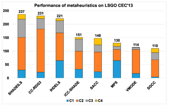
Figure 14. Average ranks of algorithms, comparison of the fine-tuned iCC-SHADE and state-of-the-art metaheuristics.

The detailed results for fine-tuned iCC-SHADE are presented in Table 17. Q1, Q2, and Q3 denotes 1.2 × 10⁵, 6.0 × 10⁵, and 3.0 × 10⁶ FEVs, respectively. The table contains the best, the median, the worst, the mean, and the standard deviation from 25 independent runs. As we can see, differences between the median and the mean values on all problems are low. The standard deviation values are less than the median and mean values in all experiments, thus the scatter of the results is not high. We can conclude that iCC-SHADE is a rather robust algorithm.

Table 17. Detailed results for the fine-tuned iCC-SHADE algorithm.

	F1	F2	F3	F4	F5	F6	F7	F8
Q1	2.32 × 109	1.02 × 104	2.14 × 10	1.30 × 1011	7.24 × 106	1.06 × 106	1.66 × 109	3.33 × 1015
	2.86 × 109	1.05 × 104	2.14 × 10	4.52 × 1011	8.56 × 106	1.06 × 106	2.84 × 109	7.77 × 1015
	3.11 × 109	1.07 × 104	2.14 × 10	9.97 × 1011	1.01 × 107	1.06 × 106	4.41 × 109	1.35 × 1016
	2.86 × 109	1.05 × 104	2.14 × 10	4.92 × 1011	8.71 × 106	1.06 × 106	3.00 × 109	7.93 × 1015
	2.11 × 108	1.27 × 102	4.86 × 10−3	2.14 × 1011	7.57 × 105	1.26 × 103	7.82 × 108	2.76 × 1015
Q2	1.47 × 103	1.02 × 103	2.12 × 10	2.22 × 1010	1.48 × 106	1.06 × 106	6.28 × 107	4.69 × 1014
	2.96 × 103	1.49 × 103	2.12 × 10	6.61 × 1010	2.57 × 106	1.06 × 106	1.84 × 108	1.07 × 1015
	7.55 × 103	2.09 × 103	2.12 × 10	1.22 × 1011	6.41 × 106	1.06 × 106	7.22 × 108	2.63 × 1015
	3.21 × 103	1.51 × 103	2.12 × 10	6.53 × 1010	2.77 × 106	1.06 × 106	2.49 × 108	1.16 × 1015
	1.57 × 103	2.96 × 102	7.87 × 10−3	2.67 × 1010	1.18 × 106	1.43 × 103	1.89 × 108	4.98 × 1014
Q3	1.32 × 10−18	8.35 × 102	2.05 × 10	2.90 × 108	1.48 × 106	1.05 × 106	4.65 × 104	2.85 × 1011
	6.77 × 10−18	9.35 × 102	2.07 × 10	7.87 × 108	2.53 × 106	1.06 × 106	2.56 × 105	1.26 × 1012
	6.72 × 10−17	1.03 × 103	2.08 × 10	3.37 × 109	3.84 × 106	1.06 × 106	6.63 × 105	1.25 × 1013
	1.01 × 10−17	9.37 × 102	2.07 × 10	9.71 × 108	2.47 × 106	1.06 × 106	2.70 × 105	2.84 × 1012
	1.29 × 10−17	3.87 × 10	3.93 × 10−2	6.81 × 108	5.78 × 105	1.75 × 103	1.38 × 105	3.30 × 1012
	F9	F10	F11	F12	F13	F14	F15
Q1	5.86 × 108	9.33 × 107	7.05 × 1010	2.56 × 109	8.31 × 1010	5.31 × 1011	4.40 × 107
	6.75 × 108	9.42 × 107	2.74 × 1011	3.09 × 109	1.12 × 1011	9.88 × 1011	6.32 × 107
	8.06 × 108	9.51 × 107	1.47 × 1012	3.84 × 109	1.34 × 1011	1.53 × 1012	9.31 × 107
	6.80 × 108	9.41 × 107	3.09 × 1011	3.15 × 109	1.09 × 1011	9.96 × 1011	6.47 × 107
	5.64 × 107	4.42 × 105	2.72 × 1011	2.91 × 108	1.54 × 1010	2.73 × 1011	1.32 × 107
Q2	1.26 × 108	9.26 × 107	8.42 × 108	1.73 × 103	3.03 × 109	5.56 × 109	3.29 × 106
	1.70 × 108	9.37 × 107	8.23 × 109	2.11 × 103	5.17 × 109	5.10 × 1010	4.30 × 106
	2.22 × 108	9.43 × 107	1.10 × 1011	2.82 × 103	1.00 × 1010	1.58 × 1011	6.80 × 106
	1.69 × 108	9.36 × 107	2.56 × 1010	2.10 × 103	5.67 × 109	5.54 × 1010	4.66 × 106
	2.63 × 107	4.60 × 105	3.01 × 1010	2.52 × 102	1.83 × 109	3.70 × 1010	9.99 × 105
Q3	1.24 × 108	9.25 × 107	6.29 × 106	9.75 × 102	6.23 × 106	1.66 × 107	1.84 × 105
	1.68 × 108	9.33 × 107	1.48 × 107	1.14 × 103	1.20 × 107	3.28 × 107	2.62 × 105
	2.18 × 108	9.37 × 107	4.13 × 107	1.43 × 103	3.72 × 107	7.88 × 107	3.29 × 105
	1.66 × 108	9.32 × 107	1.94 × 107	1.14 × 103	1.41 × 107	3.38 × 107	2.63 × 105
	2.59 × 107	3.64 × 105	1.12 × 107	1.00 × 102	7.38 × 106	1.31 × 107	3.73 × 104

5. Conclusions

In this study, the iCC-SHADE algorithm has been proposed for solving large-scale global optimization problems. iCC-SHADE dynamically changes the number of subcomponents and gradually increases the number of variables in subcomponents. The experimental results have shown that the strategy can improve the performance of the iCC-SHADE algorithm. The proposed metaheuristic has been investigated using the LSGO CEC’13 benchmark set with 15 problems. The iCC-SHADE algorithm outperforms, on average, all variants of CC-SHADE with fixed numbers of subcomponents on all LSGO CEC’13 problems. Also, iCC-SHADE demonstrates better performance, on average, in solving partially additively separable and overlapping high-dimensional problems. iCC-SHADE has been compared with seven state-of-the-art metaheuristics. The numerical results indicate that the proposed iCC-SHADE algorithm is an efficient and competitive algorithm to tackle LSGO problems. All experiments are proven by Wilcoxon test. iCC has a high potential for enhancement. The structure and specifications of our computational cluster have been presented. We have discussed the importance of applying the computational cluster in investigating the performance of evolutionary algorithms when solving LSGO problems.

In our further works, we will apply a self-adaptive approach for tuning the algorithm’s parameters. A self-adaptive approach can be applied for online tuning the number of subcomponents and the population size for each problem during the optimization process. Our hypothesis is that such a problem-specific tuning will increase the performance of the proposed iCC-SHADE algorithm.

References

- Xue, B.; Zhang, M.; Browne, W.N.; Yao, X. A Survey on Evolutionary Computation Approaches to Feature Selection. IEEE Trans. Evol. Comput. 2016, 20, 606–626. [Google Scholar] [CrossRef]
- Kicinger, R.; Arciszewski, T.; de Jong, K. Evolutionary computation and structural design: A survey of the state-of-the-art. Comput. Struct. 2005, 83, 1943–1978. [Google Scholar] [CrossRef]
- Yar, M.H.; Rahmati, V.; Oskouei, H.R.D. A Survey on Evolutionary Computation: Methods and Their Applications in Engineering. Mod. Appl. Sci. 2016, 10, 131. [Google Scholar] [CrossRef]
- Koza, T.; Karaboga, N.; Kockanat, S. Aort valve Doppler signal noise elimination using IIR filter designed with ABC algorithm. In Proceedings of the 2012 International Symposium on Innovations in Intelligent Systems and Applications, Trabzon, Turkey, 2–4 July 2012; pp. 1–5. [Google Scholar] [CrossRef]
- Thangavel, K.; Velayutham, C. Mammogram Image Analysis: Bio-inspired Computational Approach. In Proceedings of the International Conference on Soft Computing for Problem Solving (SocProS 2011), New Delhi, India, 20–22 December 2011; pp. 941–955. [Google Scholar]
- Afifi, F.; Anuar, N.B.; Shamshirband, S.; Choo, K.-K.R. DyHAP: Dynamic Hybrid ANFIS-PSO Approach for Predicting Mobile Malware. PLoS ONE 2016, 11, e0162627. [Google Scholar] [CrossRef] [PubMed]
- Nogueira-Collazo, M.; Porras, C.C.; Fernandez-Leiva, A.J. Competitive Algorithms for Coevolving Both Game Content and AI. A Case Study: Planet Wars. IEEE Trans. Comput. Intell. AI Games 2015, 8, 325–337. [Google Scholar] [CrossRef]
- Molina, D.; Moreno-Garcia, F.; Herrera, F. Analysis among winners of different IEEE CEC competitions on real-parameters optimization: Is there always improvement? In Proceedings of the IEEE Congress on Evolutionary Computation (CEC), San Sebastián, Spain, 5–8 June 2017; pp. 805–812. [Google Scholar] [CrossRef]
- Skvorc, U.; Eftimov, T.; Korosec, P. CEC Real-Parameter Optimization Competitions: Progress from 2013 to 2018. In Proceedings of the 2019 IEEE Congress on Evolutionary Computation (CEC), Wellington, New Zealand, 10–13 June 2019; pp. 3126–3133. [Google Scholar] [CrossRef]
- Tang, K.; Li, X.; Suganthan, P.; Yang, Z.; Weise, T. Benchmark Functions for the CEC’2010 Special Session and Competition on Large-Scale; Nanyang Technological University: Singapore, 2009; pp. 1–23. [Google Scholar]
- Chen, S.; Montgomery, J.; Bolufé-Röhler, A. Measuring the curse of dimensionality and its effects on particle swarm optimization and differential evolution. Appl. Intell. 2014, 42, 514–526. [Google Scholar] [CrossRef]
- Mahdavi, S.; Shiri, M.E.; Rahnamayan, S. Metaheuristics in large-scale global continues optimization: A survey. Inf. Sci. 2015, 295, 407–428. [Google Scholar] [CrossRef]
- Potter, M.A. The Design and Analysis of a Computational Model of Cooperative Coevolution. Ph.D. Thesis, George Mason University, Fairfax, VA, USA, 1997. [Google Scholar]
- Črepinšek, M.; Liu, S.-H.; Mernik, M. Exploration and exploitation in evolutionary algorithms. ACM Comput. Surv. 2013, 45, 1–33. [Google Scholar] [CrossRef]
- Vakhnin, A.; Sopov, E. Improving DE-based cooperative coevolution for constrained large-scale global optimization problems using an increasing grouping strategy. IOP Conf. Ser. Mater. Sci. Eng. 2020, 734, 012099. [Google Scholar] [CrossRef]
- Vakhnin, A.; Sopov, E. Investigation of the iCC Framework Performance for Solving Constrained LSGO Problems. Algorithms 2020, 13, 108. [Google Scholar] [CrossRef]
- Vakhnin, A.; Sopov, E. Using the iCC framework for solving unconstrained LSGO problems. IOP Conf. Series Mater. Sci. Eng. 2021, 1047, 012085. [Google Scholar] [CrossRef]
- Potter, M.A.; de Jong, K.A. A cooperative coevolutionary approach to function optimization. In Proceedings of the International Conference on Parallel Problem Solving from Nature 1994, Jerusalem, Israel, 9 October 1994; pp. 249–257. [Google Scholar]
- De Oca, M.A.M.; Aydın, D.; Stützle, T. An incremental particle swarm for large-scale continuous optimization problems: An example of tuning-in-the-loop (re)design of optimization algorithms. Soft Comput. 2010, 15, 2233–2255. [Google Scholar] [CrossRef]
- Chowdhury, J.G.; Chowdhury, A.; Sur, A. Large Scale Optimization Based on Co-ordinated Bacterial Dynamics and Opposite Numbers. In Computer Vision; Springer Science and Business Media LLC: London, UK, 2012; Volume 7677, pp. 770–777. [Google Scholar]
- Fan, J.; Wang, J.; Han, M. Cooperative Coevolution for Large-Scale Optimization Based on Kernel Fuzzy Clustering and Variable Trust Region Methods. IEEE Trans. Fuzzy Syst. 2013, 22, 829–839. [Google Scholar] [CrossRef]
- Wang, H.; Rahnamayan, S.; Wu, Z. Parallel differential evolution with self-adapting control parameters and generalized opposition-based learning for solving high-dimensional optimization problems. J. Parallel Distrib. Comput. 2013, 73, 62–73. [Google Scholar] [CrossRef]
- Takahama, T.; Sakai, S. Large scale optimization by differential evolution with landscape modality detection and a diversity archive. In Proceedings of the 2012 IEEE Congress on Evolutionary Computation, Brisbane, Australia, 10–15 June 2012; pp. 1–8. [Google Scholar]
- Marcelino, C.; Almeida, P.; Pedreira, C.; Caroalha, L.; Wanner, E. Applying C-DEEPSO to Solve Large Scale Global Optimization Problems. In Proceedings of the 2018 IEEE Congress on Evolutionary Computation (CEC), Rio de Janeiro, Brazil, 8–13 July 2018; pp. 1–6. [Google Scholar]
- Omidvar, M.N.; Li, X.; Yang, Z.; Yao, X. Cooperative Co-evolution for large scale optimization through more frequent random grouping. In Proceedings of the IEEE Congress on Evolutionary Computation, Barcelona, Spain, 18–23 July 2010; pp. 1–8. [Google Scholar] [CrossRef]
- Omidvar, M.N.; Li, X.; Mei, Y.; Yao, X. Cooperative Co-Evolution with Differential Grouping for Large Scale Optimization. IEEE Trans. Evol. Comput. 2014, 18, 378–393. [Google Scholar] [CrossRef]
- Li, X.; Tang, K.; Omidvar, M.N.; Yang, Z.; Qin, K. Benchmark Functions for the CEC’2013 Special Session and Competition on Large-Scale Global Optimization. Gene 2013, 7, 8. [Google Scholar]
- van den Bergh, F.; Engelbrecht, A. A Cooperative Approach to Particle Swarm Optimization. IEEE Trans. Evol. Comput. 2004, 8, 225–239. [Google Scholar] [CrossRef]
- El-Abd, M. A cooperative approach to The Artificial Bee Colony algorithm. In Proceedings of the IEEE Congress on Evolutionary Computation, Barcelona, Spain, 18–23 July 2010; pp. 1–5. [Google Scholar] [CrossRef]
- Shi, Y.-J.; Teng, H.-F.; Li, Z.-Q. Cooperative Coevolutionary Differential Evolution for Function Optimization. Lect. Notes Comput. Sci. 2005, 1080–1088. [Google Scholar] [CrossRef]
- Chen, H.; Zhu, Y.; Hu, K.; He, X.; Niu, B. Cooperative Approaches to Bacterial Foraging Optimization. In International Conference on Intelligent Computing; Springer: Berlin/Heidelberg, Germany, 2008; pp. 541–548. [Google Scholar] [CrossRef]
- Yang, Z.; Tang, K.; Yao, X. Multilevel cooperative coevolution for large scale optimization. In Proceedings of the 2008 IEEE Congress on Evolutionary Computation (IEEE World Congress on Computational Intelligence), Hong Kong, China, 1–6 June 2008; pp. 1663–1670. [Google Scholar] [CrossRef]
- Yang, Z.; Tang, K.; Yao, X. Large scale evolutionary optimization using cooperative coevolution. Inf. Sci. 2008, 178, 2985–2999. [Google Scholar] [CrossRef]
- Li, X.; Yao, X. Cooperatively Coevolving Particle Swarms for Large Scale Optimization. IEEE Trans. Evol. Comput. 2012, 16, 210–224. [Google Scholar] [CrossRef]
- Ray, T.; Yao, X. A cooperative coevolutionary algorithm with Correlation based Adaptive Variable Partitioning. In Proceedings of the 2009 IEEE Congress on Evolutionary Computation, Trondheim, Norway, 18–21 May 2009; pp. 983–989. [Google Scholar]
- Omidvar, M.N.; Li, X.; Yao, X. Smart use of computational resources based on contribution for cooperative co-evolutionary algorithms. In Proceedings of the 13th Annual Conference on Genetic and Evolutionary Computation, Dublin, Ireland, 12–16 July 2011; pp. 1115–1122. [Google Scholar]
- Liu, J.; Tang, K. Scaling Up Covariance Matrix Adaptation Evolution Strategy Using Cooperative Coevolution. Trans. Petri Nets and Other Models Concurr. XV 2013, 350–357. [Google Scholar] [CrossRef]
- Xue, X.; Zhang, K.; Li, R.; Zhang, L.; Yao, C.; Wang, J.; Yao, J. A topology-based single-pool decomposition framework for large-scale global optimization. Appl. Soft Comput. 2020, 92, 106295. [Google Scholar] [CrossRef]
- Li, L.; Fang, W.; Mei, Y.; Wang, Q. Cooperative coevolution for large-scale global optimization based on fuzzy decomposition. Soft Comput. 2021, 25, 3593–3608. [Google Scholar] [CrossRef]
- Wu, X.; Wang, Y.; Liu, J.; Fan, N. A New Hybrid Algorithm for Solving Large Scale Global Optimization Problems. IEEE Access 2019, 7, 103354–103364. [Google Scholar] [CrossRef]
- Ren, Z.; Chen, A.; Wang, M.; Yang, Y.; Liang, Y.; Shang, K. Bi-Hierarchical Cooperative Coevolution for Large Scale Global Optimization. IEEE Access 2020, 8, 41913–41928. [Google Scholar] [CrossRef]
- Yang, Z.; Tang, K.; Yao, X. Self-adaptive differential evolution with neighborhood search. In Proceedings of the 2008 IEEE Congress on Evolutionary Computation (IEEE World Congress on Computational Intelligence), Hong Kong, China, 1–6 June 2008; pp. 1110–1116. [Google Scholar] [CrossRef]
- Sun, Y.; Kirley, M.; Halgamuge, S.K. Extended Differential Grouping for Large Scale Global Optimization with Direct and Indirect Variable Interactions. In Proceedings of the 2015 Annual Conference on Genetic and Evolutionary Computation, Madrid, Spain, 11–15 July 2015; pp. 313–320. [Google Scholar] [CrossRef]
- Eberhart, R.C.; Kennedy, J. A new optimizer using particle swarm theory. In Proceedings of the Sixth International Symposium on Micro Machine and Human Science, Nagoya, Japan, 4–6 October 1995; pp. 39–43. [Google Scholar]
- Tanabe, R.; Fukunaga, A. Success-history based parameter adaptation for Differential Evolution. In Proceedings of the 2013 IEEE Congress on Evolutionary Computation, Cancun, Mexico, 20–23 June 2013; pp. 71–78. [Google Scholar]
- Zhang, J.; Sanderson, A.C. JADE: Adaptive Differential Evolution with Optional External Archive. IEEE Trans. Evol. Comput. 2009, 13, 945–958. [Google Scholar] [CrossRef]
- Wang, Y.; Cai, Z.; Zhang, Q. Differential Evolution with Composite Trial Vector Generation Strategies and Control Parameters. IEEE Trans. Evol. Comput. 2011, 15, 55–66. [Google Scholar] [CrossRef]
- Mallipeddi, R.; Suganthan, P.; Pan, Q.; Tasgetiren, M. Differential evolution algorithm with ensemble of parameters and mutation strategies. Appl. Soft Comput. 2011, 11, 1679–1696. [Google Scholar] [CrossRef]
- Brest, J.; Maučec, M.S. Population size reduction for the differential evolution algorithm. Appl. Intell. 2007, 29, 228–247. [Google Scholar] [CrossRef]
- Gropp, W. MPICH2: A New Start for MPI Implementations. In Proceedings of the Recent Advances in Parallel Virtual Machine and Message Passing Interface, 9th European PVM/MPI Users’ Group Meeting, Linz, Austria, 29 September–2 October 2002; p. 7. [Google Scholar] [CrossRef]
- Molina, D.; Latorre, A.; Herrera, F. SHADE with Iterative Local Search for Large-Scale Global Optimization. In Proceedings of the 2018 IEEE Congress on Evolutionary Computation (CEC), Rio de Janeiro, Brazil, 8–13 July 2018; pp. 1–8. [Google Scholar]
- Sun, Y.; Li, X.; Ernst, A.; Omidvar, M.N. Decomposition for Large-scale Optimization Problems with Overlapping Components. In Proceedings of the 2019 IEEE Congress on Evolutionary Computation (CEC), Wellington, New Zealand, 10–13 June 2019; pp. 326–333. [Google Scholar]
- Molina, D.; Herrera, F. Iterative hybridization of DE with local search for the CEC’2015 special session on large scale global optimization. In Proceedings of the 2015 IEEE Congress on Evolutionary Computation, Sendai, Japan, 24–28 May 2015; pp. 1974–1978. [Google Scholar]
- Wei, F.; Wang, Y.; Huo, Y. Smoothing and auxiliary functions based cooperative coevolution for global optimization. In Proceedings of the 2013 IEEE Congress on Evolutionary Computation, Cancun, Mexico, 20–23 June 2013; pp. 2736–2741. [Google Scholar]
- Bolufe-Rohler, A.; Chen, S.; Tamayo-Vera, D. An Analysis of Minimum Population Search on Large Scale Global Optimization. In Proceedings of the 2019 IEEE Congress on Evolutionary Computation (CEC), Wellington, New Zealand, 10–13 June 2019; pp. 1228–1235. [Google Scholar] [CrossRef]
- López, E.; Puris, A.; Bello, R. Vmode: A hybrid metaheuristic for the solution of large scale optimization problems. Inv. Oper. 2015, 36, 232–239. [Google Scholar]
- Liu, W.; Zhou, Y.; Li, B.; Tang, K. Cooperative Co-evolution with Soft Grouping for Large Scale Global Optimization. In Proceedings of the 2019 IEEE Congress on Evolutionary Computation (CEC), Wellington, New Zealand, 10–13 June 2019; pp. 318–325. [Google Scholar] [CrossRef]
Publisher’s Note: MDPI stays neutral with regard to jurisdictional claims in published maps and institutional affiliations. |
© 2021 by the authors. Licensee MDPI, Basel, Switzerland. This article is an open access article distributed under the terms and conditions of the Creative Commons Attribution (CC BY) license (https://creativecommons.org/licenses/by/4.0/).