Article

A Federated Generalized Linear Model for Privacy-Preserving Analysis

Netherlands Comprehensive Cancer Organization (IKNL), 5612 HZ Eindhoven, The Netherlands
*
Author to whom correspondence should be addressed.
Algorithms 2022, 15(7), 243; https://doi.org/10.3390/a15070243
Submission received: 14 June 2022 / Revised: 5 July 2022 / Accepted: 11 July 2022 / Published: 13 July 2022
(This article belongs to the Special Issue Interpretability, Accountability and Robustness in Machine Learning)

Abstract

:
In the last few years, federated learning (FL) has emerged as a novel alternative for analyzing data spread across different parties without needing to centralize them. In order to increase the adoption of FL, there is a need to develop more algorithms that can be deployed under this novel privacy-preserving paradigm. In this paper, we present our federated generalized linear model (GLM) for horizontally partitioned data. It allows generating models of different families (linear, Poisson, logistic) without disclosing privacy-sensitive individual records. We describe its algorithm (which can be implemented in the user’s platform of choice) and compare the obtained federated models against their centralized counterpart, which were mathematically equivalent. We also validated their execution time with increasing numbers of records and involved parties. We show that our federated GLM is accurate enough to be used for the privacy-preserving analysis of horizontally partitioned data in real-life scenarios. Further development of this type of algorithm has the potential to make FL a much more common practice among researchers.

1. Introduction

1.1. Federated Learning

In the past few years, there has been a surge in the amount of potential data available for gathering [1]. Machine learning (ML) and artificial intelligence (AI) have leveraged this and have allowed the development of numerous analytic tools across many different industries, such as healthcare, banking, and manufacturing, among many others [2,3,4,5].
Due to the inherent complex nature of systems and processes, data are usually fragmented in silos across parties. For example, parties could have collected different data features for the same group of individuals (i.e., vertically partitioned data). Alternatively, parties could have gathered the same features but for a different group of individuals (i.e., horizontally partitioned data) [6]—the latter being the focus of this work.
In the traditional way of working, data fragmentation is solved by pooling the data from all parties into a single location. In other words, each party generates a copy of its data. Then, these copies are brought together and centralized by a trusted party, which then proceeds with analyzing the data and obtaining a global model. Unfortunately, this centralized approach is undesirable due to several operational, organizational, and political challenges. For example, once a copy of the data is created and is shared outside its point of origin, is very hard to keep control of it. Sometimes, the costs of integrating huge amounts of data scattered across different parties can make centralization infeasible [7]. More importantly, there are increasing privacy and security concerns and requirements that make merging the data in a single point infeasible. Users are more and more concerned that their private data are being used for commercial or political purposes without their consent [8]. Moreover, regulatory bodies all around the world have started implementing laws that regulate responsible data management and use, such as the California Consumer Privacy Act (CCPA, 2020) in California, USA and the General Data Protection Regulation (GDPR, 2018) in Europe, among many others [9,10,11].
Federated learning (FL) has emerged as an alternative paradigm to overcome these shortcomings [12]. In this approach, the process of generating the global model is distributed among the parties. Instead of sharing their data, the involved parties perform computations on them, generating aggregated statistics (often encrypted) that are then shared to generate the global model. This keeps the original data undisclosed and safe at their original location, greatly reducing the risk of leaking privacy-sensitive information while generating global models that are very close (if not practically identical) to their centralized counterparts [13].
Several ML/AI algorithms have been implemented as their corresponding federated counterparts for analyzing horizontally partitioned data [14], such as decision trees [15], support vector machines [16], hierarchical training [17], gradient boosting decision trees [18,19], logistic regression [20], Cox Proportional Hazard model [21], and neural networks [22,23], among others. However, in spite of their versatility (Section 1.2), the implementation of generalized linear models (GLMs) has received little attention.

1.2. Generalized Linear Models

The term generalized linear model (GLM) refers to a large class of models popularized by McCullagh and Nelder [24]. In these models, the response variable y i is assumed to follow an exponential family distribution with mean μ i , which is assumed to be some (often non-linear) function of x i T β .
There are three components to any GLM. First, there is the random component, which describes the probability distribution of the response variable y. We will consider only cases in which the observations come from a distribution in the exponential family with probability density function as given by Equation (1):
f ( y , θ ) = e x p y θ b ( θ ) a ( ϕ ) + c ( y , ϕ )
Here, θ is the canonical parameter (such that E ( y ) = μ = b ( θ ) and V a r ( y ) = a ( ϕ ) b ( θ ) ). It is straightforward to show that the canonical parameter for y N ( μ , σ 2 ) is θ = μ , and the canonical parameter for y B i n ( n , π ) is θ = l o g i t ( π ) = l o g π 1 π .
Secondly, there is a systematic component, which defines how the linear combination of the explanatory variables x = ( x 1 , x 2 , , x k ) define the linear predictor Equation (2), where β must be estimated:
η = x T β
Lastly, there is a link function  g ( · ) , which specifies the link between the random and the systematic components (depending on how the mean function is expressed). The most commonly used link function for a normal model is η = μ , while for a binomial model, it is η = l o g i t ( π ) . Note that whenever η = g ( μ ) = θ , we say that the model has a canonical link.

1.2.1. Estimation of a Centralized GLM

In order to estimate a GLM, we need to calculate the maximum likelihood estimation (MLE) for β . Using the canonical link η = θ , the log likelihood can be written as in Equation (3):
l = i = 1 n l o g f ( y i , θ i ) = i = 1 n y i θ i b ( θ i ) a ( ϕ ) + c ( y i , ϕ )
To find the MLE, we use Fisher’s scoring algorithm for which the generic ( t + 1 ) -th step can be calculated using Equation (4):
β ( t + 1 ) = β ( t ) + E l β ( t ) 1 l ( β ( t ) )
where l and l are the first and second derivative of the log-likelihood, which are given by Equation (5) and Equation (6), respectively:
l ( β ( t ) ) = δ l δ β j = i = 1 n δ l i δ θ i δ θ i δ μ i δ μ i δ η i δ η i δ β j = i = 1 n y i μ V a r ( y i ) δ μ i δ η i x i j
E l β ( t ) = E δ 2 l δ β j δ β k = i = 1 n 1 V a r ( y i ) δ μ i δ η i 2 x i j x i k
where x i j and x i k are the j-th and k-th element of the covariate vector for the i-th observation. Using algebra and matrix notation, we can rewrite them as Equations (7) and (8):
δ l δ β = X T A ( y μ )
E δ 2 l δ β j δ β k = X T W X
where X = ( x 1 , , x K ) T , A = d i a g V a r ( y i ) δ η i δ μ i 1 and W = d i a g V a r ( y i ) δ η i δ μ i 2 1 .
With this, the Fisher Scoring iteration of Equation (4) can be rewritten as Equation (9):
β ( t + 1 ) = β ( t ) + X T W X 1 X T A ( y μ )
and considering that X β = η and A = W δ η δ μ , we can rewrite it as Equation (10):
β ( t + 1 ) = X T W X 1 X T W z
where z = η + δ η δ μ ( y μ ) . This way, Fisher Scoring can be regarded as Iteratively Reweighted Least Squares (IRWLS) carried out on a transformed version of the response variable. The IRWLS algorithm can be described as in Algorithm 1, where g ( · ) is the link function, Δ g = δ μ δ η is the derivative of the inverse-link function g ( · ) with respect to the linear predictor, and w = w 1 , , w n are arbitrary weights assigned to the units (which equal to 1 by default).
In this paper, we present our federated implementation of a GLM for horizontally partitioned data. The manuscript is organized as follows. Section 2 describes the algorithm of the presented federated GLM in detail, how it was implemented, and its validation process for both accuracy and execution time. These results are shown in Section 3, where they are also discussed in detail. We also show examples where our federated GLM is being used as well as discuss possible improvements for it. Section 4 closes the paper with our overall conclusions.
Algorithm 1 Fisher Scoring-based Centralized GLM
1:
procedure  
2:
       initialize β ( 0 )
                        η = X β ( 0 )
                        d e v ( 0 )  
3:
       loop
4:
             compute μ = g ( η )
                              z = η + y μ Δ g
                              W = w Δ g 2 V a r ( μ )
5:
             update β ( j ) = X T W X 1 X T W z
                           η = X β ( j )
6:
             compute d e v ( j )  
7:
             if  | d e v ( j ) d e v ( j 1 ) |   <   ϵ  then
                 return  β ( j )
                 break loop
8:
             else
                  j = j + 1
9:
             end if
10:
       end loop 
11:
end procedure

2. Materials and Methods

We assume that all the involved parties have previously agreed on what variables will be used as an input to the model as well as the variable to be predicted, and they have consistently harmonized their data.

2.1. Setup

Our presented federated GLM algorithm is designed to run on a server–client architecture [6], as shown in Figure 1. In this scenario, (1) the user sends a task (i.e., the instruction to run a specific algorithm) to the server. When received, (2) the server manages and synchronizes the execution of the algorithm across all nodes (i.e., parties). In short, (3) each node accesses its own local data and executes the requested algorithm with the given parameters. Afterwards, the node outputs a set of intermediate results (often in the form of preliminary coefficients), which are sent back to the server. Then, using these, (4) the server computes a first version of the global solution and sends it back to the nodes, which use it to compute a new set of results. This process is repeated iteratively until (5) the global solution converges or after a fixed number of iterations, yielding the final version of the (federated) model.

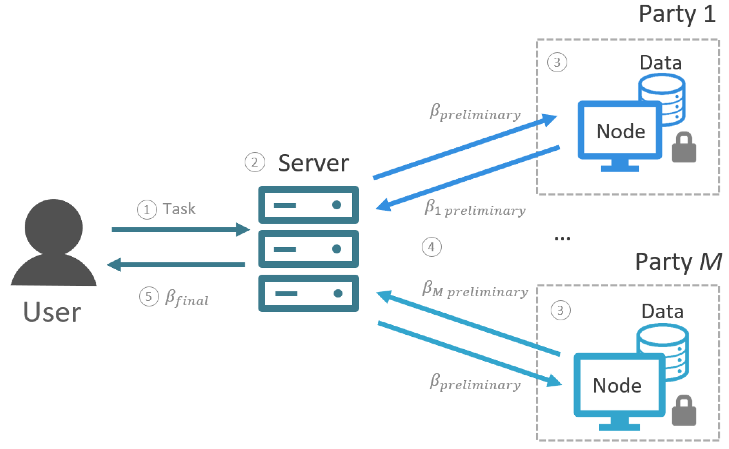
2.2. Algorithm for a Federated GLM

Here, we describe the algorithm of a federated version of the GLM model. The main idea behind it is that the components of Equation (10) can be (partially) computed at each party k and put together afterwards without ever bringing the data together.
Let us consider M 2 parties (e.g., data registries, hospitals, banks, etc.) holding an exclusive partition of the full dataset. Let us denote by n m the number of observations in the m-th data source such that the total sample size of the study is given by n = n 1 + + n M .
The first and the expected second derivatives of Equations (5) and (6) can be rewritten as in Equations (11) and (12), respectively:
l ( β ( t ) ) = m = 1 M i = 1 n m y i μ V a r ( y i ) δ μ i δ η i x i j
E l β ( t ) = m = 1 M i = 1 n m 1 V a r ( y i ) δ μ i δ η i 2 x i j x i k
Therefore, using the matrix form, we can rewrite Equation (10) as Equation (13):
β ( t + 1 ) = m = 1 M X ( m ) T W ( m ) X ( m ) 1 m = 1 M X ( m ) T W ( m ) z ( m )
where X ( m ) is the ( n m × K ) -matrix of covariates for party m, W ( m ) is the correspondent K-dimensional diagonal matrix of weights, and z m is the n m -vector of adjusted dependent variable of the m-partition.
The federated algorithm is described in Algorithm 2. Note that the proposed algorithm is mathematically equivalent to the one used for centralized data (Section 1.2.1), but it does not require the data to be pooled together.
The federated GLM was implemented in R v. 4.1.3 [25]. Its code as well as the code used for its validation (Section 2.3) is publicly available in our GitHub repository (accessed 14 June 2022).

2.3. Validation

We validated two important aspects of our federated GLM: accuracy and execution time. For both cases, we used artificial data generated using Python v. 3.8 [26]. The rest of the validation was completed using R v. 4.1.3 [25] and was performed in a laptop running Windows 10® (64 bit) with an Intel® Core i7 CPU running at 1.8 GHz and 32 GB of RAM.

2.3.1. Accuracy

In order to demonstrate the accuracy of our federated GLM, we generated three models, each from a different family (with its corresponding linking function) and with an appropriate dataset. These are summarized as follows.
Algorithm 2 Federated GLM
Initialization Server
1:
initialize β ( 0 )
Initialization Node m
2:
initialize η ( m ) = X ( m ) β ( 0 )
3:
initialize μ ( m ) = g ( η ( m ) )
4:
initialize d e v ( m ) ( 0 ) = f ( y ( m ) μ ( m ) , w ( m ) )
1:
loop 
Node m
2:
      compute z ( m ) = η ( m ) + y ( m ) μ ( m ) Δ g ( m )
3:
      compute W ( m ) = w ( m ) Δ g ( m ) 2 V a r ( μ ( m ) )
4:
      compute and return to Server X ( m ) T W ( m ) X ( m ) and X ( m ) T W ( m ) z ( m )  
Server
5:
      update β ( t + 1 ) = m = 1 M X ( m ) T W ( m ) X ( m ) 1 m = 1 M X ( m ) T W ( m ) z ( m )
6:
      return to Nodes β ( t + 1 )  
Node m
7:
      compute η ( m ) = X ( m ) β ( t + 1 )
8:
      compute μ ( m ) = g ( η ( m ) )
9:
      calculate d e v ( m ) ( t + 1 ) = f ( y ( m ) μ ( m ) , w ( m ) )
10:
     return to Server d e v ( m ) ( t + 1 )
 
Server
11:
     compute d e v ( t + 1 ) = m = 1 M d e v ( m ) ( t + 1 )
12:
     if  | d e v ( t + 1 ) d e v ( t ) | < ϵ  then
                 return  β ( t + 1 )
                 break loop
13:
     else
                  t = t + 1
14:
     end if
15:
end loop

Linear Regression

This model assumes a Gaussian distribution of the error and uses an identity link function. Notice that this particular case corresponds to that of a general linear model (not to be confused with a GLM; in other words, a general linear model is a specific case of a GLM). The target variable y was generated according to Equation (14):
y = 0.25 x 1 + 0.5 x 2 + ζ
where
x 1 = N ( 1 , 1 )
x 2 = N ( 2 , 1 )
ζ = N ( 0 , 1 )

Poisson Regression

This model assumes a Poisson distribution of the error and uses a log link function. The target variable y was generated according to Equation (18):
y = round ( e 0.25 x 1 + 0.5 x 2 + ζ )
where x 1 , x 2 , and ζ were defined the same way as in the previous model (Equation (15), Equation (16) and Equation (17), respectively).

Logistic Regression

This model assumes a binomial distribution and uses a logit link function. In this case, the data were generated using scikit-learn v. 1.0.2 [27]. They consisted of normally distributed clusters of points (with a standard deviation of 1) around vertices of a 2D plane (since we chose to use two features, x 1 and x 2 ) [28].
In all cases validating the federated GLM’s accuracy, the data comprised 3000 records, which were randomly split into three simulated parties with 1000 records each. The federated GLM was run using a mock server–client architecture. This was available from our previously developed open-source priVAcy preserviNg federaTed leArninG infrastructurE for Secure Insight Exchange—vantage6 [29]. In short, it recreated a server and the nodes of all three parties locally (which is sufficient for verifying the mathematical implementation of the algorithm), making the development and testing very practical. We set the algorithm to stop its execution if it converged (i.e., if the difference between the coefficients across iterations was smaller than 1 × 10 8 ) or if it reached 50 iterations (the latter condition was never reached; the algorithm converged in all the presented cases).
Afterwards, we compared the federated GLM output to their centralized counterpart, which can be considered the gold standard. Here, the data were all put together as if they were all available to a single party. Then, a (centralized) GLM was generated using R’s glm function from the stats package [25]. Specifically, we compared the federated and centralized models’ coefficients, standard errors, p-, and z-values. Tables were generated using the package stargazer v. 5.2.3 [30].

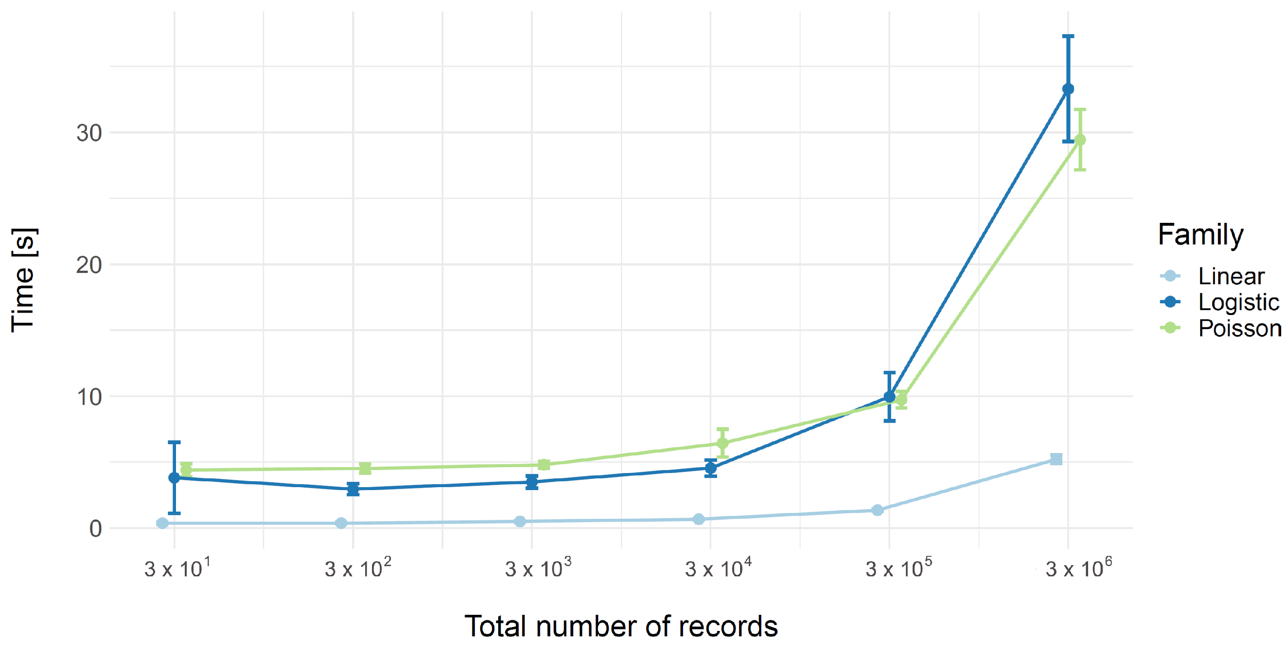
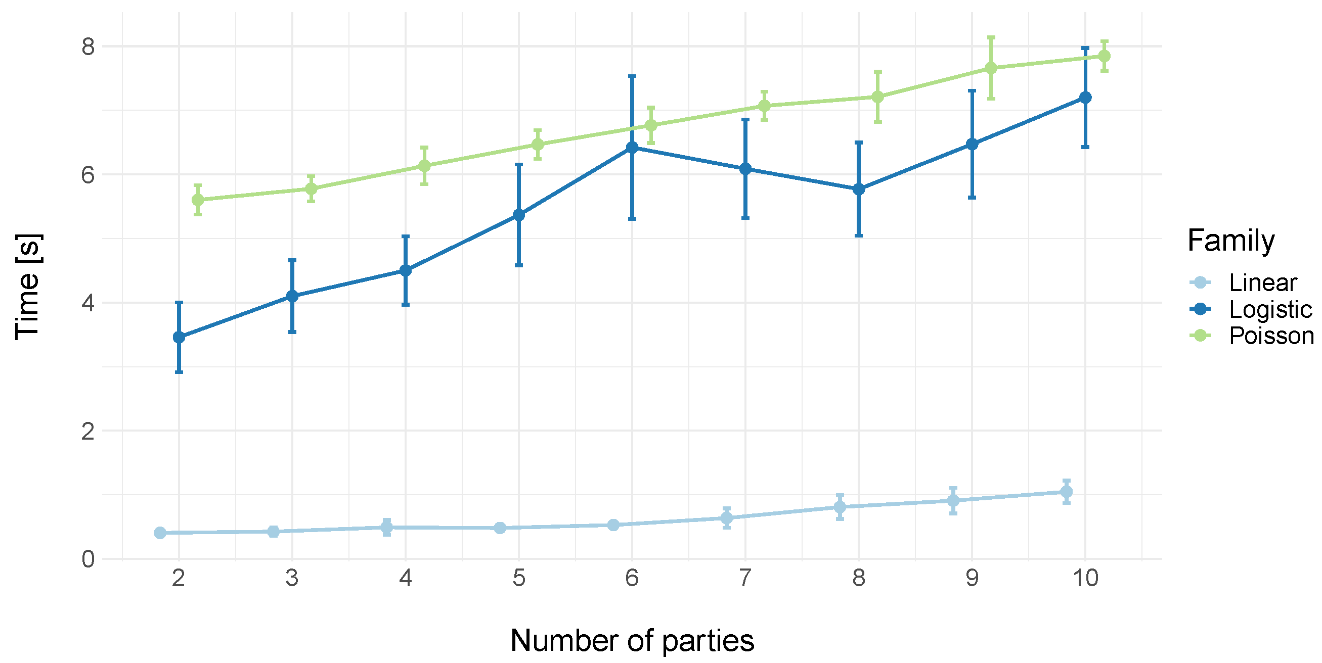
2.3.2. Execution Time

We were also interested in validating how the federated GLM’s execution time escalates under different circumstances. For this purpose, we ran numerous simulations. All of them used the same mock server–client architecture and parameters described earlier.
First, we explored the impact of increasing the number of records while keeping the number of parties constant. Using the same corresponding data for each family as before, we simulated a total of 30, 300, …, 3,000,000 records in a three-party scenario (i.e., each party had 10, 100, …, 1,000,000 records).
Afterwards, we explored the impact of increasing the number of parties while keeping the number of records constant. Using the same setup as before, we simulated scenarios with 2 , 3 , , 10  parties with a total of 10,000 records. Records were distributed randomly and practically evenly among parties (e.g., in a three-party scenario, two parties would have 3333 records, while the remaining one would have 3334).
In both of these validations, in order to obtain a proper idea of the performance and to account for the variability due to inherent randomness in the data generation process, each case was simulated 100 times. We only measured the time (in seconds) from the beginning to the end of the federated GLM execution. In other words, we discarded the time it took to generate the data, since in a real-life situation, each party would already have their own data at hand.

3. Results and Discussion

Table 1 shows a comparison between the results of the centralized and the federated GLMs. We can see that in all cases, the output of both types of models is practically identical. This demonstrates that our implementation of a federated GLM is capable of generating an equivalent model of that using a centralized approach but without the need of sharing any data among the involved parties.
After this, we were confident that the results of our federated GLM were practically identical to those of its centralized counterpart. Thus, we proceeded to validate its execution time.
Figure 2 shows the execution time as a function of the total number of records in a fixed three-party scenario. For all three families, we can see that the execution time remains relatively constant from 30 until 30,000 records. In this case, the execution time of the linear model is ∼0.5 s, while for both logistic and Poisson families, it is ∼5 s. However, there is a large increase after that, with the linear family having approximately a 10 × increase reaching ∼5 s and the logistic and Poisson families having approximately a 6 × increase reaching ∼30 s.
Figure 3 shows the execution time as a function of the number of parties while keeping the total number of records constant (at 10,000). We can see that for all three families, there is a constant increase in execution time as a function of the number of parties. This makes sense, since a larger number of parties implies a larger number of communications between them and the server for each iteration of the algorithm. The linear family still remains as the fastest model by far, which is followed by the logistic and Poisson families.
We should mention that the execution times shown here are just indicative and can only provide an idea of how the algorithm escalates with increasing numbers of records/parties. However, these times will very likely be different when used in a real-life scenario due to a variety of reasons. First of all, this study was performed using a mock server–client architecture, which simulates a server and the nodes in a local environment. In this setup, the server–node communication is very efficient, since there is practically no overhead caused by network operations. In real life, said overhead is very likely to be larger due to low internet connection speeds, varying network infrastructures, etc., yielding a slower execution [31]. Moreover, the data used for the validation were generated artificially with relatively simple relations between variables. Real-life data can be much more complex, which can cause the algorithm to take a larger number of iterations to converge (with the possibility of not converging at all).
There are several ways that the presented federated GLM algorithm can be used in real-life analyses. If the parties have an FL infrastructure up and running, they could either implement it from scratch according to their particular needs (based on the description given on Section 2.2) or they could use our provided implementation. As mentioned earlier, this was completed in R. However, it can be used in either R or Python through the provided wrappers. If the parties do not have an FL infrastructure, the easiest way is to use it as part of vantage6. An exhaustive description of the platform is given by Moncada-Torres et al. [29] and Smits et al. [32], while its documentation can be found on its website https://vantage6.ai/ (accessed 14 June 2022).
Our federated GLM is already being used in real-life analyses. For example, it has been applied by Wenzel et al. as a logistic regression to identify women with early stage cervical cancer at low risk of lymph node metastasis. This subpopulation of women is very specific and the number of incidences tends to be quite low, making drawing conclusions from a small patient cohort difficult. In said study, the authors have used our federated GLM to generate a logistic regression that uses data from three different parties (namely, cancer registries across three different European countries). This way, they increased the number of patients for their analysis and generated a more powerful model that supports identifying women with early stage cervical cancer with a low risk of lymph node metastasis, allowing for a more conservative treatment [33,34]. In another interesting use case, Hamersma used our federated GLM as a basis for performing stratified propensity score matching [35] (which in turn reduced confounding bias by indication) between breast cancer subpopulations of two international cancer registries. Afterwards, the authors compared quality indicators between them—all of it without having to pool data together [36]. Needless to say, these are only a couple of examples where our presented federated GLM has been used. Its applications can go well beyond oncology or health care, after all.
There are a few aspects of our federated GLM that could be improved. For example, decreasing communication overhead is known to be a bottleneck for all FL applications [37]. Communication could be more efficient using parallelism in each training round [23] or by actively managing parties’ contributions based on the status of their conditions (e.g., network speeds, time required for local updates) [38]. Model update time could also be decreased by transmitting only part of the updated local model by the parties [39].

4. Conclusions

In this paper, we presented our federated GLM, which allows generating models of different families (linear, Poisson, logistic) in a privacy-preserving manner. The algorithm can be implemented in the platform of choice of the user or it can be utilized out-of-the-box using the provided implementation in our infrastructure for FL, vantage6. We validated its performance by comparing it with its centralized counterpart, which can be considered the gold standard. Given the mathematical equivalence of the two algorithms, our federated GLM reproduced outputs that are practically identical to those obtained when all the data were pooled together. We also validated its execution time as a function of the number of records and number of parties. Both validations demonstrated the usability of our federated GLM for analyzing horizontally partitioned data without disclosing information at a record level. Further development of this type of algorithm has the potential of making privacy-preserving analyses methods, such as FL, a much more common practice among researchers.

Author Contributions

Conceptualization, M.C., A.J.v.G. and A.M.-T.; methodology, M.C., A.J.v.G., H.A. and A.M.-T.; software, all authors; validation, M.C., A.J.v.G. and A.M.-T.; formal analysis, M.C., A.J.v.G. and A.M.-T.; investigation, M.C. and A.M.-T.; resources, F.M.; data curation, A.M.-T.; writing—original draft preparation, M.C. and A.M.-T.; writing—review and editing, all authors; visualization, A.M.-T.; supervision, A.M.-T.; project administration, F.M., A.M.-T. All authors have read and agreed to the published version of the manuscript.

Funding

This research received no external funding.

Data Availability Statement

The data used in this study were generated programmatically as described in the text (Section 2.3). The corresponding scripts are publicly available in our GitHub repository.

Conflicts of Interest

The authors declare no conflict of interest.

Abbreviations

The following abbreviations are used in this manuscript:
AIArtificial intelligence
FLFederated learning
GLMGeneralized linear model
MLMachine learning
MLEMaximum likelihood estimation

References

  1. Sagiroglu, S.; Sinanc, D. Big data: A review. In Proceedings of the 2013 International Conference on Collaboration Technologies and Systems (CTS), San Diego, CA, USA, 20–24 May 2013; pp. 42–47. [Google Scholar]
  2. Hatcher, W.G.; Yu, W. A survey of deep learning: Platforms, applications and emerging research trends. IEEE Access 2018, 6, 24411–24432. [Google Scholar] [CrossRef]
  3. Hassani, H.; Huang, X.; Silva, E. Digitalisation and big data mining in banking. Big Data Cogn. Comput. 2018, 2, 18. [Google Scholar] [CrossRef] [Green Version]
  4. Wuest, T.; Weimer, D.; Irgens, C.; Thoben, K.D. Machine learning in manufacturing: Advantages, challenges, and applications. Prod. Manuf. Res. 2016, 4, 23–45. [Google Scholar] [CrossRef] [Green Version]
  5. Fildes, R.; Ma, S.; Kolassa, S. Retail forecasting: Research and practice. Int. J. Forecast. 2019, 35, 1–34. [Google Scholar] [CrossRef] [Green Version]
  6. Li, L.; Fan, Y.; Tse, M.; Lin, K.Y. A review of applications in federated learning. Comput. Ind. Eng. 2020, 149, 106854. [Google Scholar] [CrossRef]
  7. Group, W.A. Federated Learning White Paper; Technical Report; WeBank AI Group: Beijing, China, 2018. [Google Scholar]
  8. Politou, E.; Alepis, E.; Patsakis, C. Forgetting personal data and revoking consent under the GDPR: Challenges and proposed solutions. J. Cybersecur. 2018, 4, tyy001. [Google Scholar] [CrossRef]
  9. van Veen, E.B. Observational health research in Europe: Understanding the General Data Protection Regulation and underlying debate. Eur. J. Cancer 2018, 104, 70–80. [Google Scholar] [CrossRef] [PubMed] [Green Version]
  10. Piper, D. Data Protection Laws of the World; Technical Report; DLA Piper: MD, USA, 2020. [Google Scholar]
  11. Bukaty, P. The California Consumer Privacy Act (CCPA): An Implementation Guide; IT Governance Ltd.: Ely, UK, 2019. [Google Scholar]
  12. Dai, W.; Wang, S.; Xiong, H.; Jiang, X. Privacy preserving federated big data analysis. In Guide to Big Data Applications; Springer: Berlin/Heidelberg, Germany, 2018; pp. 49–82. [Google Scholar]
  13. Xu, J.; Wang, F. Federated Learning for Healthcare Informatics. arXiv 2019, arXiv:1911.06270. [Google Scholar] [CrossRef] [PubMed]
  14. Zhang, C.; Xie, Y.; Bai, H.; Yu, B.; Li, W.; Gao, Y. A survey on federated learning. Knowl.-Based Syst. 2021, 216, 106775. [Google Scholar] [CrossRef]
  15. Lindell, Y.; Pinkas, B. Privacy preserving data mining. J. Cryptol. 2002, 15, 36–54. [Google Scholar] [CrossRef]
  16. Wild, E.; Mangasarian, O. Privacy-Preserving Classification of Horizontally Partitioned Data via Random Kernels; Technical Report; University of Wisconsin: Madison, WI, USA, 2007. [Google Scholar]
  17. Gao, D.; Ju, C.; Wei, X.; Liu, Y.; Chen, T.; Yang, Q. Hhhfl: Hierarchical heterogeneous horizontal federated learning for electroencephalography. arXiv 2019, arXiv:1909.05784. [Google Scholar]
  18. Tian, Z.; Zhang, R.; Hou, X.; Liu, J.; Ren, K. Federboost: Private federated learning for gbdt. arXiv 2020, arXiv:2011.02796. [Google Scholar]
  19. Zhao, L.; Ni, L.; Hu, S.; Chen, Y.; Zhou, P.; Xiao, F.; Wu, L. Inprivate digging: Enabling tree-based distributed data mining with differential privacy. In Proceedings of the IEEE INFOCOM 2018-IEEE Conference on Computer Communications, Honolulu, HI, USA, 15–19 April 2018; pp. 2087–2095. [Google Scholar]
  20. Slavkovic, A.B.; Nardi, Y.; Tibbits, M.M. “Secure” Logistic Regression of Horizontally and Vertically Partitioned Distributed Databases. In Proceedings of the Seventh IEEE International Conference on Data Mining Workshops (ICDMW 2007), Omaha, NE, USA, 28–31 October 2007; pp. 723–728. [Google Scholar]
  21. Lu, C.L.; Wang, S.; Ji, Z.; Wu, Y.; Xiong, L.; Jiang, X.; Ohno-Machado, L. WebDISCO: A web service for distributed cox model learning without patient-level data sharing. J. Am. Med. Inform. Assoc. 2015, 22, 1212–1219. [Google Scholar] [CrossRef] [PubMed] [Green Version]
  22. Bonawitz, K.; Eichner, H.; Grieskamp, W.; Huba, D.; Ingerman, A.; Ivanov, V.; Kiddon, C.; Konecny, J.; Mazzocchi, S.; McMahan, H.B.; et al. Towards Federated Learning at Scale: System Design. In Proceedings of the 2nd Conference on Systems and Machine Learning (SysML), Standford, CA, USA, 31 March–2 April 2019. [Google Scholar]
  23. McMahan, B.; Moore, E.; Ramage, D.; Hampson, S.; y Arcas, B.A. Communication-efficient learning of deep networks from decentralized data. In Proceedings of the Artificial Intelligence and Statistics, PMLR, Fort Lauderdale, FL, USA, 20–22 April 2017; pp. 1273–1282. [Google Scholar]
  24. McCullagh, P.; Nelder, J.A. Generalized Linear Models; Routledge: London, UK, 2019. [Google Scholar]
  25. R Core Team. R: A Language and Environment for Statistical Computing; R Foundation for Statistical Computing: Vienna, Austria, 2022. [Google Scholar]
  26. Van Rossum, G.; Drake, F.L. Python 3 Reference Manual; Python Software Foundation: DE, USA, 2009. [Google Scholar]
  27. Pedregosa, F.; Varoquaux, G.; Gramfort, A.; Michel, V.; Thirion, B.; Grisel, O.; Blondel, M.; Prettenhofer, P.; Weiss, R.; Dubourg, V.; et al. Scikit-learn: Machine Learning in Python. J. Mach. Learn. Res. 2011, 12, 2825–2830. [Google Scholar]
  28. Guyon, I.; Gunn, S.; Ben-Hur, A.; Dror, G. Result analysis of the NIPS 2003 feature selection challenge. Adv. Neural Inf. Process. Syst. 2004, 17, 1–8. [Google Scholar]
  29. Moncada-Torres, A.; Martin, F.; Sieswerda, M.; van Soest, J.; Geleijnse, G. VANTAGE6: An open source priVAcy preserviNg federaTed leArninG infrastructurE for Secure Insight eXchange. In Proceedings of the AMIA Annual Symposium Proceedings, Online, 14–18 November 2020; pp. 870–877. [Google Scholar]
  30. Hlavac, M. stargazer: Well-Formatted Regression and Summary Statistics Tables; R Package Version 5.2.3; Social Policy Institute: Bratislava, Slovakia, 2022. [Google Scholar]
  31. Hartmann, F. Federated Learning. Master’s Thesis, Frei Universität Berlin, Berlin, Germany, 2018. [Google Scholar]
  32. Smits, D.; van Beusekom, B.; Martin, F.; Veen, L.; Geleijnse, G.; Moncada-Torres, A. An Improved Infrastructure for Privacy-Preserving Analysis of Patient Data. In Proceedings of the International Conference of Informatics, Management, and Technology in Healthcare (ICIMTH), Athens, Greece, 1 July–3 July 2022; Volume 295, pp. 144–147. [Google Scholar]
  33. Wenzel, H.H.; Norberg Hardie, A.; Bekkers, R.L.; Falconer, H.; Hogdall, C.K.; Jensen, P.T.; Lemmens, V.E.; Martin, F.; van Gestel, A.J.; Moncada-Torres, A.; et al. Using Federated Learning to Identify Women with Early Stage Cervical Cancer at Low Risk For Lymph Node Metastases. 2022; under review. [Google Scholar]
  34. Wenzel, H. Improving Quality of Cervical Cancer Care with (Inter)National Cancer Registry Data. Ph.D. Thesis, University of Groningen, Groningen, The Netherlands, 2022. [Google Scholar]
  35. Rosenbaum, P.R.; Rubin, D.B. The central role of the propensity score in observational studies for causal effects. Biometrika 1983, 70, 41–55. [Google Scholar] [CrossRef]
  36. Hamersma, D.T. A Comparison of the Quality of Breast Cancer Care in Norway and The Netherlands. Master’s Thesis, University of Twente, Enschede, The Netherlands, 2020. [Google Scholar]
  37. Yang, Q.; Liu, Y.; Chen, T.; Tong, Y. Federated machine learning: Concept and applications. ACM Trans. Intell. Syst. Technol. (TIST) 2019, 10, 12. [Google Scholar] [CrossRef]
  38. Nishio, T.; Yonetani, R. Client selection for federated learning with heterogeneous resources in mobile edge. In Proceedings of the ICC 2019–2019 IEEE International Conference on Communications (ICC), Shanghai, China, 20–24 May 2019; pp. 1–7. [Google Scholar]
  39. Konečnỳ, J.; McMahan, H.B.; Yu, F.X.; Richtárik, P.; Suresh, A.T.; Bacon, D. Federated learning: Strategies for improving communication efficiency. arXiv 2016, arXiv:1610.05492. [Google Scholar]
Figure 1. Required server–client architecture needed for executing the presented federated GLM algorithm. Notice that the data never leave their corresponding party.
Algorithms 15 00243 g001
Figure 2. Execution time for the different families (linear, Poisson, logistic) of the GLM. In this case, the number of parties was kept constant (at 3), while the total number of records went from 30 to 3,000,000 with increasing order of magnitude. Thus, the scale of the x-axis is logarithmic. Each scenario was simulated 100 times. Data points represent the mean of the execution time, while error bars represent ±1 standard deviation. The lines of each family were slightly shifted along the x-axis to avoid overlap between them.
Algorithms 15 00243 g002
Figure 3. Execution time for the different families (linear, Poisson, logistic) of the GLM. In this case, the number of records was kept constant (at 10,000), while the number of parties was 2, 3, …, 10. Each scenario was simulated 100 times. Data points represent the mean of the execution time, while error bars represent ±1 standard deviation. The lines of each family were slightly shifted along the x-axis to avoid overlap between them.
Algorithms 15 00243 g003
Table 1. Comparison of the centralized vs. federated GLMs.
FamilyParameterCoefficientsStd. Errorp-Valuesz-Values
CFCFCFCF
Linear(Intercept) 0.069 0.069 0.045 0.045 0.129 0.129 1.520 1.520
x 1 0.221 0.221 0.017 0.017 00 12.763 12.763
x 2 0.499 0.499 0.018 0.018 00 27.212 27.212
Poisson(Intercept) 0.595 0.595 0.021 0.021 00 28.465 28.465
x 1 0.269 0.269 0.007 0.007 00 37.220 37.220
x 2 0.446 0.446 0.007 0.007 00 62.566 62.566
Logistic(Intercept) 0.104 0.104 0.064 0.064 0.106 0.106 1.617 1.617
x 1 2.593 2.593 0.093 0.093 00 27.802 27.802
x 2 0.054 0.054 0.051 0.051 0.291 0.291 1.055 1.055
C: centralized; F: federated.
Publisher’s Note: MDPI stays neutral with regard to jurisdictional claims in published maps and institutional affiliations.

