1. Introduction
A heat speared problem handles the estimate of unidentified numbers appearing in the mathematics of physical in thermal knowledges, by means of the dimensions or measurement of the temperature, radiation intensities, heat flux, etc.
The inverse problem for the heat PDE system can be solved by many methods; for example, the method of Tikhonov [
1], the method of Lavrentiev [
2], Ivanov [
3], and many others. The inverse problems in the heat PDE system can be grouped as two types depending on the e unknown function or vector for the initial part or the boundary part conditions, and many studies of these problems are considered in many works [
4,
5,
6,
7,
8,
9,
10,
11,
12]. Various methods for solving this type of inverse problem have been proposed in many works [
13,
14,
15,
16,
17]. In the article [
13], the BVP for the PDE heat equation in a hollow cylinder was solved by using the Fourier projection method. Papers [
14,
16] studied the multigrid method with the iterative method to find the solution for the inverse problem, IP, in the heat PDE system. In [
15,
17], the iterative methods with necessary analyses were studied for solving the inverse linear operator equation and the case study in this paper was the inverse heat PDE system problem.
The successfully accomplished approaches for resolving the IPs are dependent, to a large degree, on the deep insight into the mathematical problems related to the algorithms and statements and the definition of the specific difficulties in their solving [
18,
19,
20,
21,
22,
23].
The goal of this article is to provide the approximation solution for the BVP in the PDE for the heat equation system with the mixed interval for time. Hence, the result of this problem (BVP) is not contingent continuously on the known data in the field, which means the solution is not stable; therefore, this problem is known as an ill-posed inverse problem. The proving of the boundary function of this problem belonged to the class necessary for applying the projection regularization method by using the Fourier transform. For solving the ill-posed problems, a central role is played by the error estimations between the approximation and real solutions. We obtain the estimate solution by applying the projection regularization method with the Fourier transform, making these results new and interesting.
2. Materials and Methods Direct Formulation of the Problem on Interval
We considered the case of the heat equation on a segment with inhomogeneous boundary data.
Assume the
function is defined as the following
by using Duhamel’s principle method ([
24], p. 109)
integration by parts for the right part for (6) once, we obtain
Now, we can decide to obtain the solution for
as the following
by substituting (8) in (7), to obtain a solution to a non-stationary problem, from (5)
where
, and
Lemma 1. Letsatisfy condition (5). Then, there exists a solutionfor problem (1)–(5) such thatsatisfies the Equation (1) on the set, initial condition (2), boundary conditions (3), (4) and
Proof. By integrating the right side of the Formula (10) in parts twice, we obtain
since
for any
and from the Cauchy–Bunyakovsky inequality
by means of (5), (4) and (12) for any
and for any
we obtain
Using Equations (11)–(13) and convergence of the series , , with the Weierstrass criterion follows the unchanging convergence of the above series on .
Since the functions
, obtaining
Thus, with
and
in addition to Equations (11) and (14), we take
. From this condition and the convergence of (19) in domain
, we have
. Differentiating a
with
and by using (13), we obtain
From the above relation, we obtain the convergence of the in , from (8) we have in and .
Now, let us examine the function .
Differentiating the function by twice and using (11), we obtain since the number series , converge according to the Weierstrass criterion, the functional series converge absolutely and uniformly on .
Then, we need to check the convergence for to any in this series, related to the Dirichlet criterion, the convergence is consistently on .
Meanwhile, any
series
converges on
and the parts of this series are nonstop, we obtain
The lemma is proofed. □
Now, let us examine the function .
Lemma 2. Function, defined by formulas (9) and (11), belongs to space.
Proof. From (5), (9) and (11) it follows that
where
Since the conditions
are right, then, form (15) and (16) by means of the Weierstrass criterion which leads to the convergence of the series, therefore
We will show that
. From (16) and (17), we obtain
From (12), it follows that
Third series
absolutely converges on
then
. □
3. Expansion of the Direct Problem (1)–(5) on
Let us study the following PDE system in the interval
.
We obtain the following solution by applying the separation of variables as a way for solving problem (18)–(21)
where
By integrating the right side of (24) twice, we obtain
From (22) and (25), we define a number
such that for any
From (23) and (26), any
then,
Let us consider there exists the numbers
and
such that for any
and, it follows from (30) and (31), that
then, it follows from (18), (27)–(32) that there is
known as a number such that for any
Now, let us examine the behavior ,
Lemma 3. Letbe defined by the formula (24). Thenwhereis the fourth derivative with respect tofor function.
Proof. defined by the Equation (24), and integrating
in parts twice, we obtain
from (3) and (19)
Since
as a result, we obtain
Integrating the right part of the previous equation twice in parts, it leads to
The lemma is proofed. □
From Lemmas 2 and 3, the series
; hence, from (23), we obtain
Denote , from (34) and (35), it follows that
Lemma 4. Let the functionbe defined by Equation (34). Then,such that for any Proof. From (34) and (35), it follows that
where
some number.
Let us assume that
and
From
it follows that, for
and numbers
,
from (36), it follows that
. Hence there is a number
for any
from (35) and Lemma 4, it follows that
Now, let us introduce the notation
From (33) and (37), it follows that, for any
there is
which is defined as a function such that, for any
where
Since , then the Fourier transform for can be used for the combined direct problem (1)–(5) and (18)–(21).
The lemma is proofed. □
From Lemma 1 and Equation (38), we obtain the following theorem.
Theorem 1. Letandis limited over this line. Then, the following relations are true Lemma 5. Letbe a solution of the combined problem (1)–(5) and (18)–(21). Then, the following relations are true.
Proof. It follows from Lemma 1 and (35) that, for any
Let the number
be defined by the formula
Then, let us denote by
the function defined by the formula
Since
and for any
then, given (39); by the Lebesgue theorem on the passage to the limit under the integral sign, the assertion of the lemma is proved. □
4. Solution of the Inverse BVPs (1)–(5) and (18)–(21)
Let us assume that the function in the combined problem (1)–(5) and (18)–(21) is unknown, and, instead, the function is given as , where .
Let us adopt that, for
, there is a function
such that, when it is substituted into the boundary of (1)–(5) and (18)–(21), we obtain a real solution
which is defined as the following
Function
unknown, and, instead, we have
and
such that
It is necessary to use the given data and inverse BVP (1)–(5) and (18)–(21) in order to find an approximate solution and obtain an error estimate
5. Solution of the Inverse BVP (1)–(5) and (18)–(21) by the Projection Regularization Method
Let
be the interval on the area of complex numbers, and the set of correction class
demarcated by the following
known positive number.
In order to resolve the problem (1)–(5) and (18)–(21), we present
, as the operator which is mapping from
to
and we named as the operator via the Fourier transform
There —interval on the of complex numbers set.
Denote by operator continuation in . Following from Plancherel’s theorem, the operator has isometric mapping into .
Let
. Then, we have
where the way to the limit has the sense of the convergence of root-mean-square.
Using transform
, (1)–(5) and (18)–(21) come down to the following problem
where
Solutions (45) and (46) are of the form
where
and
are functions that satisfy (40) and (46).
With
we obtain
Therefore, the problem (45) and (46) reduces to the equation
Let
and, from the Formula (41), it follows that
Let
denote a set of
such that
and
Since , then .
In order to find the approximation solution for (49)–(51) we use the regularizing family of operators
, which are defined by
For selecting a regularization parameter in Equation (52) from the initial data , use the equation .
Let us describe an estimated solution for (49) by the formulation of .
This follows from the theorem formulated in the article [
25] [c. 284], that
where
Let us describe
as the operator for use in the regularization method in order to obtain the approximate solution for the problem. (49) in
. Now, let us introduce
as the quantitative characteristic of the accuracy of this method on the set
.
From the theorem proved in [
23], it follows that the following estimate holds
From (51) and (55), we obtain for .
Lemma 6. Let. Then, forthe ratio is true
Lemma 6 tracks from the explanation of the operator norm. According to [
26], lemma 2, to compute the modulus of continuity,
we need to solve
Solving
is replaced into the function
parameter determined by
From (56) and (57), it follows that
Therefore, from (53), (57) and (58), we obtain the estimate
In order to simplify the assessment (59), consider the equations
Let and , respectively, be solutions of the Equation (60).
Then, from (56), (60), we find that, for sufficiently small
, defined
, the following relations are valid
where
,
and, from the resulting inequality, we have
From the theorem proved in [
26], it follows that
where
from (54) we find that this is an exact ordinal estimate,
From lemma 5, (53) and (63) we obtain
Theorem 2. For methodwe have an exact estimate of the order error
Applying к
transformation
where
is the inverse Fourier transform operator, we obtain an estimated solution for the problem (1)–(5) and (18)–(21).
Thus, for an approximate solution
for problem (1)–(5) and (18)–(21), we have a precise error estimation by
6. Case Study
Consider the function suppose .
From the solution of the direct problem (1)–(5) and (18)–(21), we find
We set a partition of the time interval
with the number of nodes
such that
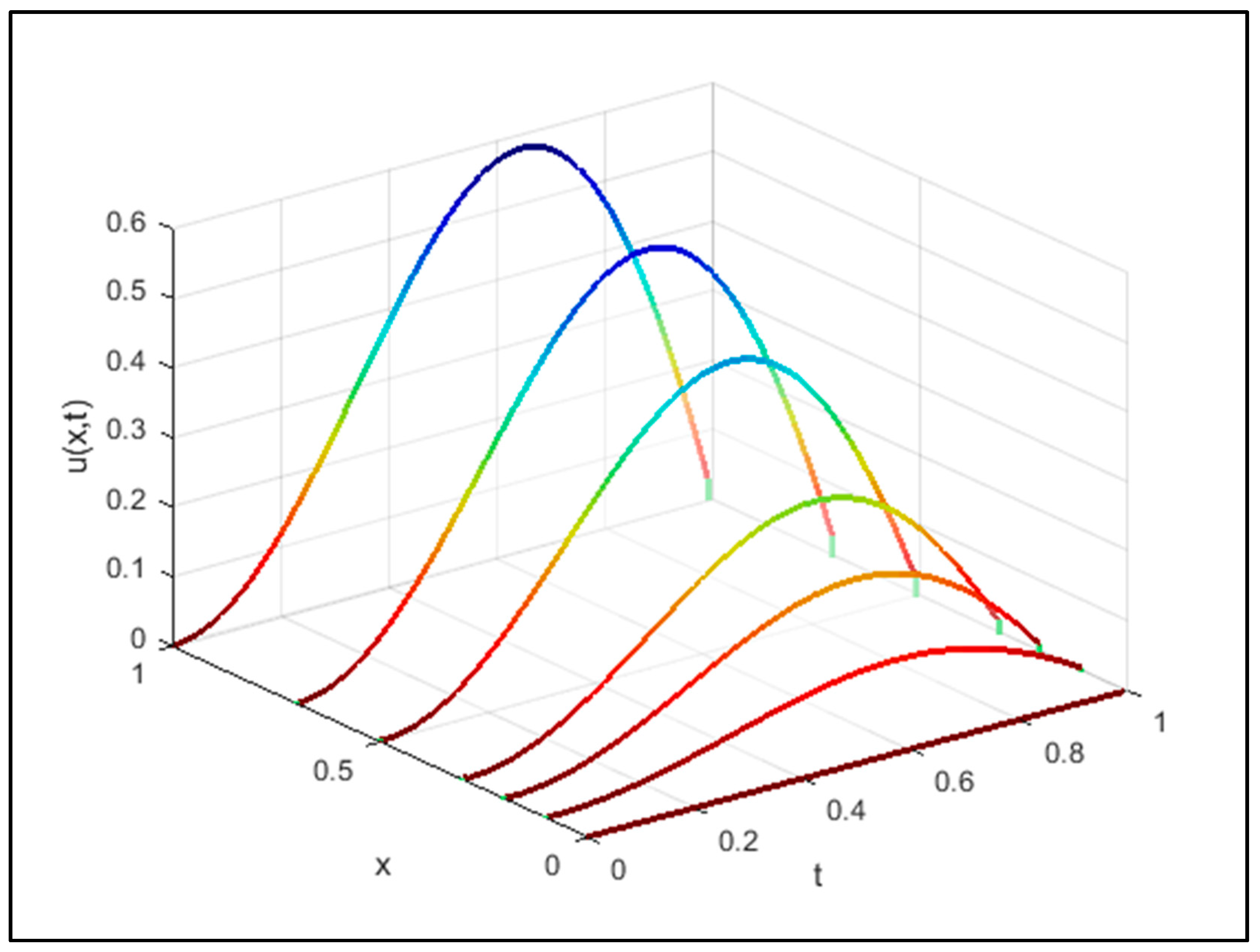
This simulates the one-dimensional nature of the heat equation using the Fast Fourier Transform, FFT, as shown in
Figure 1. In this example, the PDE system is linear, and it is possible to advance the system directly in the frequency domain.
From
Figure 1 we find
, introducing an error level
and
in
by the following
where the error level can compute by
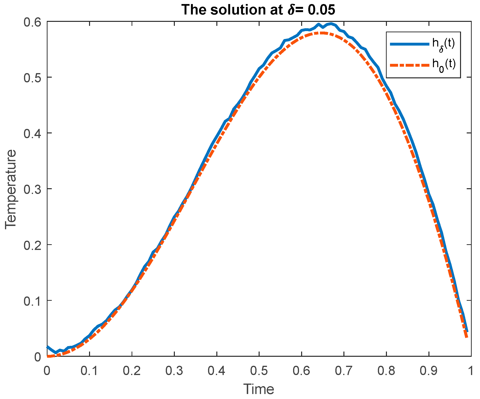
Figure 2 and
Figure 3 show the visualization of the function as a solution for the inverse problem with
and
, respectively. The real solution is shown by a dotted line and the approximate solution is shown by a line.


 ,
, 


