Abstract
Ant colony optimization (ACO) is a well-known class of swarm intelligence algorithms suitable for solving many NP-hard problems. An important component of such algorithms is a record of pheromone trails that reflect colonies’ experiences with previously constructed solutions of the problem instance that is being solved. By using pheromones, the algorithm builds a probabilistic model that is exploited for constructing new and, hopefully, better solutions. Traditionally, there are two different strategies for updating pheromone trails. The best-so-far strategy (global best) is rather greedy and can cause a too-fast convergence of the algorithm toward some suboptimal solutions. The other strategy is named iteration best and it promotes exploration and slower convergence, which is sometimes too slow and lacks focus. To allow better adaptability of ant colony optimization algorithms we use κ-best, max-κ-best, and 1/λ-best strategies that form the entire spectrum of strategies between best-so-far and iteration best and go beyond. Selecting a suitable strategy depends on the type of problem, parameters, heuristic information, and conditions in which the ACO is used. In this research, we use two representative combinatorial NP-hard problems, the symmetric traveling salesman problem (TSP) and the asymmetric traveling salesman problem (ATSP), for which very effective heuristic information is widely known, to empirically analyze the influence of strategies on the algorithmic performance. The experiments are carried out on 45 TSP and 47 ATSP instances by using the MAX-MIN ant system variant of ACO with and without local optimizations, with each problem instance repeated 101 times for 24 different pheromone reinforcement strategies. The results show that, by using adjustable pheromone reinforcement strategies, the MMAS outperformed in a large majority of cases the MMAS with classical strategies.
1. Introduction
Ant colony optimization (ACO) is a nature-inspired metaheuristic that has been used as a design template for many successful algorithms. These algorithms are mostly used to solve NP-hard combinatorial optimization problems, although ACO has also been used for continuous and mixed-variable optimization problems [,,,,,]. ACO algorithms are stochastic and cannot guarantee optimal solutions, but they are commonly applied to NP-hard optimization problems because, for such problems, exact algorithms generally cannot yield optimal solutions in a reasonable time. It is sometimes also possible to combine ACO techniques like pheromone trails with Monte Carlo methods to maintain some advantages from both procedures [].
The key concept in ACO is the use of pheromone trails associated with solution components to allow the colony of artificial ants to accumulate collective knowledge and experience about the problem instance that they are trying to solve. These pheromone trails bias future attempts of artificial ants to construct better solutions. Being metaheuristic, ACO only gives general recipes on how to devise an algorithm. For solving a specific type of problem, it is necessary to devise a specific ACO algorithm, and success depends not only on the nature of the problem but also greatly on how these recipes are applied. It is important to enable good guidance in the search space by properly balancing between exploration and exploitation. A too greedy algorithm might result in fast convergence toward moderate or bad solutions, but too little greediness can result in slow convergence or unguided roaming through search space with a very low probability of obtaining good solutions. For some NP-hard problems, ACO can get substantial help from heuristic information, but for other NP-hard problems such useful heuristic information is unknown or maybe impossible. Heuristic information is very useful for problems where some kind of optimal route is objective, such as the traveling salesman problem (TSP) [], asymmetric traveling salesman problem (ATSP) [], sequential ordering problem (SOP) [,], various vehicle routing problems (VRPs) [,], car renter salesman problem (CaRS) [], etc. In these cases, the searching process can be faster because of heuristic information, and thus, the parameters and strategies used in ACO should be adjusted accordingly.
The standard methods for reinforcing pheromone trails in modern ACO variants have diametrically opposite strategies, leaving a large gap between too much and too little greediness. In this paper, we conduct experimental research on generalized reinforcement strategies to gain better control over algorithmic behavior and, thus, achieve better performance in ant colony optimization algorithms. The research questions that we tried to answer were the following. Can adjustable pheromone reinforcement strategies improve the algorithmic performance of ACO algorithms? How can κ-best and max-κ-best be generalized or extended to provide less greedy algorithmic behavior than with κ = 1, in the case when this is desirable? How do different adjustable pheromone strategies influence the behavior of ACO algorithms (with and without local optimization) for combinatorial problems that have efficient heuristic information? For experiments performed to answer these research questions, we have chosen well-known instances of TSP and ATSP. Initial ideas for such strategies were presented at the conference [], and here, we extend our proposal and carry out a comprehensive experimental evaluation. The results show that, by using adjustable reinforcement strategies, an ACO algorithm can obtain better solutions and allow greater control over algorithmic behavior. The main contributions of this paper are a novel 1/λ-best strategy and comprehensive experimental research that answered previously stated research questions and provided insight into what influence the adjustable pheromone strategies have on the algorithmic behavior of ACO, thus expanding scientific knowledge about ACO.
The remainder of this paper is structured as follows. After the relevant related work is covered in Section 2, Section 3 explains combinatorial problems that are relevant to this study and important to understand the MAX-MIN ant system explained in Section 4. Section 5 explains the numerically adjustable strategies κ-best, max-κ-best, and 1/λ-best. Section 6 gives details about experimental settings and procedures, while Section 7 presents the results of the experiments. Finally, the discussion is given in Section 8.
2. Related Work
Improvements made by ant colony optimization variants are achieved by changing either the solution construction procedure or the pheromone update procedure. In the case of a solution construction procedure, almost all ACO algorithms use the random proportional rule introduced by the ant system [,] or the more general variant, the pseudo-random proportional rule, used by the ant colony system []. Many improvements in ant colony optimization variants are based on changing the way the pheromone trails are modified in the pheromone update procedure. These changes are more often concerned with the way the pheromone trails are reinforced than with the way the pheromone trails are evaporated.
The initial variant of ACO, named the ant system [], uses all solutions from the current iteration in the pheromone reinforcement procedure. The components of better solutions are proportionally reinforced with more pheromone value than the solutions with worse quality. This type of strategy provides only little guidance to the subsequent solution construction procedure in searching through the solution space. The pheromone reinforcement strategy introduced by the ant system causes too much exploration and too little exploitation of previous knowledge.
In an attempt to improve algorithmic behavior, an ACO variant named the elitist ant system was proposed []. To make the algorithm greedier, in addition to pheromone reinforcement of all solutions in the current iteration, the components of the best solution found from the beginning of the algorithm (also called global-best solution) are reinforced with a weight determined by the parameter e.
More selective in choosing solutions for pheromone reinforcement is the rank-based ant system, which uses weights for pheromone reinforcement based on solution ranks and reinforces only w solutions from the current iteration [], where w is an integer parameter.
Modern variants of the ACO algorithms use only one solution, in some sense “the best” solution, to reinforce pheromone trails. The ant colony system (ACS) uses the global-best solution for pheromone reinforcement []. The MAX-MIN ant system (MMAS) uses the iteration-best or global-best solution [].
The most commonly used variant of ACO is probably the MMAS because of its excellent performance on many combinatorial optimization problems. When a faster and greedier variant is preferred, then ACS might be used instead of MMAS.
The best–worst ant system uses only the global-best solution to reinforce pheromone trails but also decreases the pheromone trails associated with the components of the worst solution in the current iteration that are not contained in the global-best solution [,].
Although the authors of BWAS claimed good performance, the BWAS algorithm did not gain wide popularity.
Population-based ant colony optimization uses the iteration-best solution to reinforce pheromone trails but also has a special mechanism to completely unmake the pheromone reinforcement made in the previous iteration, which is especially suitable for dynamic optimization problems [,].
There are also some studies about reinforcing pheromone trails that cannot be applied in general cases and address only specific situations. In [], Deng et al. proposed a technique for situations when pheromone trails are associated with nodes instead of arcs of the construction graph. The best-so-far strategy is used together with new rules (these new rules are named r-best-node update rule and a relevant-node depositing rule; the first one has a somewhat similar name to our κ-best strategy, although the actual methods are very different) proposed by the authors specifically for this type of problem. Their approach is applied to the shortest path problem, even though the path is not uniquely defined by the set of nodes and, therefore, pheromone trails associated with arcs would seem a more appropriate choice. Associating pheromone trails to nodes in the shortest path problem might have some success only if a path has a small subset of all possible nodes.
Pheromone modification strategies are proposed for dynamic optimization problems [,]. These strategies are not related to pheromone reinforcement, but instead, they are about reacting to the change in problem to avoid restarting the algorithm. The pheromone trails are modified to recognize changes in the problem instance, which is applicable in cases where changes are small or medium.
Rather complex rules for giving weights to additional pheromone values used in the pheromone reinforcement procedure of ACS are proposed in []. The authors performed an experimental evaluation of the proposed rules on three small instances of Euclidean TSP and claim better results than those obtained by AS and standard ACS.
The pheromone update strategy that is based on the theory of learning automata, where additional pheromone values for reinforcement procedure depend not only on solution quality but also on current pheromone trails, is used in [].
Swarm intelligence approaches are successfully combined with machine learning, forming together a novel research field that has provided some outstanding results in different areas [,].
3. Combinatorial Optimization Problems Relevant to This Study
Ant colony optimization always uses pheromone trails and, for some problems, heuristic information to guide the ant’s construction of a particular solution. For some problems, useful heuristic information was not discovered. For example, in the case of the quadratic assignment problem (QAP) one of the best-performing variants of the ACO algorithm, the MAX-MIN ant system, does not use heuristic information. Other examples of NP-hard problems for which successful ACO algorithms do not use heuristic information are the shortest common supersequence problem (SCSP) [] and the maximum clique problem (MCP) [].
For some problems, researchers discovered heuristic information that can significantly guide and speed up the search process and, thus, improve the performance of ACO algorithms. This includes the traveling salesman problem (TSP), asymmetric traveling salesman problem (ATSP), sequential ordering problem (SOP), vehicle routing problem with time window constraints (VRPTW) [], car renter salesman problem (CaRS), and many others. For example, by using heuristic information (with parameter β = 4) for TSP problem instance pka379, one ant in ACO can increase the probability of obtaining a particular optimal solution in the first iteration by an enormous 1.03 × 10719 times. Since TSP with 379 nodes has 378!/2 = 3.28 × 10811 solutions, this probability is increased from 3.05 × 10−812 without heuristic information to 3.14 × 10−93 with heuristic information. It is obvious that, when considering those probabilities, we never expect to obtain an optimal solution in the first iteration of the algorithm, but heuristic information can help tremendously in starting iterations of ACO algorithms [].
We used TSP and ATSP for experimental investigation in this research as they are often used for testing new techniques or strategies of the swarm and evolutionary computation algorithms and have various interesting extensions like SOP, VRPTW, and CaRS.
The asymmetric traveling salesman problem can be defined using a weighted directed graph with a set of vertices V and a set of arcs A. The objective is to visit all vertices exactly once and return to the starting vertex while minimizing the total tour weight. All the information needed to solve the problem can be stored in a matrix that specifies the distance between vertices in each direction (e.g., because of one-way streets).
The symmetric variant of the problem, where dij = dji, is traditionally studied separately, is denoted simply as TSP. The symmetric TSP is possibly one of the most researched NP-hard problems with significant achievements for some special variants. After decades of research for the metric variant of TSP and especially Euclidian TSP, there are specialized heuristics that can efficiently solve rather large instances, often to an optimum. In metric TSP, there is a constraint that, for any three nodes labeled as i, j, and k, the following triangle inequality holds:
In addition, for Euclidian TSP, it is true that for any two nodes i and j with coordinates (xi, yi,), (xj, yj) the distance dij is given by:
In this context, metaheuristics usually use metric and Euclidean TSP instances for testing new techniques and strategies and less commonly to produce the best performing algorithm for such variants.
4. MAX-MIN Ant System for TSP and ATSP
It is important to note that ACO is a general metaheuristic that has different variants, and among them, the important variants are the ant colony system (ACS) [,], MAX-MIN ant system (MMAS) [], and three bound ant system (TBAS) [,]. Since MMAS is very successful and the most popular for these kinds of optimization problems, in this study, we describe and use the MMAS variant. The general description of the MMAS metaheuristic is given in Algorithm 1. In the initialization phase, the algorithm loads the problem instance and parameter settings and creates and initials necessary variables and data structures such as pheromone trails, solutions, etc.
| Algorithm 1: A high-level description of MMAS. |
| INPUT: problem instance, parameter settings (including stopping criteria and local optimization choice) Initialize (); FirstIteration = true; While stopping criteria are not met do For each ant k in the colony do Sk = ConstructSolution(); If local optimization is enabled then Sk = LocalOptimization (Sk); EndIf If fist ant in the colony then Sb = Sk; EndIf EndFor If FirstIteration is true then Solution = Sb; FirstIteration = false; Else if Sb is better than Solution then Solution = Sb; EndIf EvaporatePheromoneTrails(); ReinforcePheromoneTrails(); EndWhile |
| OUTPUT: Solution |
Our implementation of MMAS for ATSP and TSP uses a common design and associates each arc with distance dij to pheromone trail τij and organizes it in a matrix. After that, in the while loop, the colony of ants constructs new solutions. If some kind of local optimization is used, which is optional, then solutions are possibly improved according to the implemented method. After that, pheromone trails are evaporated by using the equation:
i.e., by multiplying each pheromone trail with 1 − ρ, where ρ is a parameter of the algorithm that must be between 0 and 1. If the pheromone value drops below the lower limit τMIN, then the pheromone trail is set to τMIN. After the pheromone trails are evaporated, the trails associated with components of some kind of best solutions are reinforced in the ReinforcePheromoneTrails () procedure. These pheromone trails that are reinforced are increased in MMAS for TSP and ATSP by using Equation (4):
where is the cost of some kind of best solution, which is normally the best solution in the current iteration or best solution so far (in all previous and current iteration). If the case of TSP when pheromone trail τij is reinforced, then by symmetry is also set τji = τij.
5. Adjustable Pheromone Reinforcement Strategies
As explained in Section 4, after each iteration of the ACO algorithm, pheromone trails are updated by using some kind of best solution. In historical ACO algorithms like the ant system, all solutions from the current iteration were used to reinforce pheromone trails. This kind of strategy did not get good performance and was suppressed by modern ACO algorithms that use the iteration-best or global-best strategy. In the iteration-best strategy, only the best solution is used for pheromone reinforcement, and in global best (also called best-so-far), the best solution from the beginning of the algorithm is used. These two strategies have very different levels of greediness (focus on exploitation), and the optimal level would often be somewhere in between. In some cases, researchers try to alternate these two strategies in different scheduling. For example, three times the iteration-best (ib), then one time the global-best (gb) solution, and then repeat this in cycles. For this kind of scheduling strategy, further on we use notations such as 3-1-ib-gb.
To allow the entire spectrum of strategies that are adjustable by a numerical parameter, we have given our initial proposals κ-best strategies and max-κ-best strategies in a short conference paper []. Parameter κ is an integer value between 1 and infinity, and the larger the parameter κ is, accordingly, the greediness (exploitation) increases. Unfortunately, there were some errors in the conducted experiment (bug in the program) that favored more greedy strategies, and thus, the experimental results of that paper should be discarded. Meanwhile, we have used these strategies in different situations to get better results for MMAS and TBAS algorithms. We also noticed that the optimal value for parameter κ was sometimes 1, so here, we propose another strategy whose greediness (exploitation) is less than 1-best and max-1-best. This new strategy is called 1/λ-best and should be less greedy with a larger λ value and, hence, less greedy with a smaller number 1/λ, which extends the κ-best and max-κ-best strategies. All three strategies are defined in the following subsections.
5.1. Reinforcement Strategy κ-Best
This strategy uses the best solution constructed in the last κ iterations, where the parameter κ can be any number from the set of natural numbers {1, 2, 3, 4, 5, …} or infinity. To implement this strategy, it is necessary to have a data structure that can store up to κ solutions. In each new iteration, the iteration-best solution should be added to that data structure. Before adding a new solution, it is necessary to check how many solutions are already in the data structure. If the data structure already stored the maximum-allowed κ solutions, then the oldest solution should be removed first. In addition, if the new solution is better than all the solutions found in the given structure, all the older solutions can be safely removed. A suitable data structure for storing solutions in such a way is a queue, as shown in Figure 1. It allows adding the newest and removing the oldest element with O(1) complexity and also finding the best solution in the queue with O(κ) complexity. Because the time and space complexity of this strategy is linear with respect to parameter κ, very big values of κ are not practical because they would have a negative effect on algorithmic speed. However, we do not expect very different behavior from the algorithm that uses the 100-best and 1000-best strategies because different handling of reinforcement solution would happen only in the cases when the algorithm neither improved nor reconstructed the solution found before 100 iterations. Taking into consideration the inner working of ACO algorithms, this is a rather unlikely event that should rarely happen, thus making 100-best and 1000-best very similar strategies. Special cases of κ-best are 1-best, which is equivalent to the iteration-best strategy, and strategies with large values of κ that are larger than the maximal number of allowed iterations for the algorithm. Those large κ strategies, such as the ∞-best strategy, are equivalent to the global-best strategy since they use the best solution from all previous iterations. Although strategies with very large κ values that must be implemented with a queue are generally not efficient because of linear complexity, those large enough to be equivalent to global best are efficiently implemented with O(1) complexity by storing only one solution that is best so far.
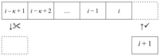
Figure 1.
Inserting and removing solutions from queue in κ-best strategy.
5.2. Reinforcement Strategy Max-κ-Best
In the max-κ-best strategy, the best solution that was found can be used in up to κ iterations of the algorithm. Then, after κ iterations, if the algorithm fails to find a better solution, it takes the best solution from the last iteration and uses it for pheromone reinforcement. The data structure for this strategy is simple and consists of one solution and one integer type of counter. At the beginning of the algorithm, in the initialization phase, the counter variable should be set to 0. After each iteration, the best solution from that iteration, ibSolution, enters the max-κ-best strategy, as shown in Figure 2. The same as with the κ-best strategy, there are two special cases. The max-1-best is equivalent to the iteration-best strategy, and for κ larger than the maximal number of iterations, this strategy is equivalent to the global-best strategy.
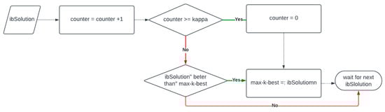
Figure 2.
Adding iteration-best solution to max-κ-strategy.
5.3. Reinforcement Strategy 1/λ-Best
This is the strategy that uses the λ solutions that are best from the last iteration of the ACO algorithm. We chose to write it as a fraction 1/λ, so this way the larger the lambda gets, the smaller the value of the fraction is, and this fits nicely as a complementary method for κ-best. So in both strategies, a smaller number means less greedy (less exploitation), and a large number means more greedy (more exploitation). The special case is where λ = 1, and then the strategy becomes 1/1-best, which is equivalent to the κ-best strategy 1-best. The maximal value that λ could obtain is the number of solutions constructed in one iteration (number of ants in the colony), which would correspond to the strategy used in the ant system (AS).
6. Experimental Settings
For experiments, we have implemented MMAS for TSP and ATSP both with and without local optimization in C++. For TSP, implemented local optimization was the 2-opt that always accepts the first improvement gained by 2-exchange. For ATSP, we used 2.5-opt also with the first improvement. For all algorithms, the parameter α was set to 1; for problem instances of size 100 or more, the favorite list size was set to 30, and an initial value for the pheromone trail was set according to the following equation:
where f(snn) is the cost of an approximate solution obtained by the nearest neighbor heuristic, and the upper trail limit τMAX was set equal to τ0. For MMAS algorithms without local optimization, the colony size m was set equal to the size of the problem n, β was set to 4, and ρ was set to 0.02, while for MMAS algorithms with local optimization, the colony size m was set equal to 25, β was set to 2, and ρ to 0.2. These parameters are recommended in the literature for MMAS designed for TSP and ATSP [,].
For each problem instance, we tested 24 pheromone reinforcement strategies: 1/5-best, 1/4-best, 1/3-best, 1/2-best, 2-best, 4-best, 8-best, 16-best, 32-best, 64-best, 128-best, max-2-best, max-4-best, max-8-best, max-16-best, max-32-best, max-64-best, max-128-best, 5-1-ib-gb, 3-1-ib-gb, 2-1-ib-gb, 1-1-ib-gb, iteration-best = 1/1-best = 1-best = max-1-best, and global-best = ∞-best = max-∞-best. Each experiment was allowed 10,000 iterations, and each experiment was repeated 101 times. All together, 7.05 × 10¹¹ solutions were constructed by MMASs, not counting changes achieved by local optimization. The experiments were conducted on computer cluster Isabella.
For TSP, we used well-known problem instances available in TSPLIB (TSPLIB collection of TSP instances is publicly available at http://comopt.ifi.uni-heidelberg.de/software/TSPLIB95/, accessed on 1 April 2023) and VLSI Data Sets (VLSI Data Sets collection of TSP instances is publicly available at https://www.math.uwaterloo.ca/tsp/vlsi/, accessed on 1 April 2023), and for ATSP instances from 8th DIMACS Implementation Challenges (ATSP instances from 8th DIMACS Implementation Challenge are publicly available at http://dimacs.rutgers.edu/archive/Challenges/TSP/atsp.html, accessed on 1 April 2023). Their characteristics and stopping criteria for MMAS without local optimization and for MMAS with 2-opt local optimization are listed in Table 1 and Table 2.

Table 1.
Information per problem instance in the case of MMAS for TSP without local optimization and with 2-opt local optimization.
Table 2.
Information per problem instance in the case of MMAS for ATSP without local optimization and with 2.5-opt local optimization.
7. Results
The results of experiments are analyzed by using medians as a suitable measure of average algorithmic performance [,]. It is worth noting that for a single execution of the MMAS algorithm, which is stochastic by nature, there is at least a 50% probability of obtaining a solution that is as good as the median solution or even better than that. By multiple running of the MMAS algorithm, whether sequentially or in parallel, it is possible to arbitrarily increase this probability of getting a solution at least as good as the median solution. For five executions, the probability becomes 96.88%, which is rather high, or by 10 executions with a very high probability of 99.9% [].
Although for each experiment the stopping criteria were limited to 10,000 iterations, in the case of the MMAS algorithm with some smaller problem instances, this was obviously unnecessarily too many iterations. With some strategies, the MMAS found optimal solutions within much fewer iterations in all 101 repetitions, while with other strategies, this was achieved after many more iterations. Therefore, after collecting results, we determined for each problem instance the number of iterations after which we performed analyses of the results using the following method. We tracked the best median solution from 10,000 iterations backward until we reached the iteration at which this median solution (out of 101 samples) was reached by at least one of 24 strategies. This iteration was rounded up to the nearest hundred, after which we analyzed the obtained solution quality. So, for example, when MMAS without local optimization was used for gr21, then after 100 iterations the analysis was performed, but in the case of u574, the analysis was performed only after 9800 iterations, as presented in Table 1. The same method was used for ATSP, and the iterations after which the analyses were performed are listed in Table 2, along with other data about problem instances.
The median values out of 101 samples were calculated for each strategy and problem instance after the selected number of iterations, as presented in Table 1 and Table 2. The median results achieved by four MMAS algorithms are presented in Figure 3, Figure 4, Figure 5 and Figure 6. These figures contain a combination of graphical and tabular forms. For each problem instance (first column), the size is given in the second column. The third column has a percentage deviation from the optimum for the median solution achieved by the best strategy, and the fourth column has a percentage deviation from the optimum for the median solution achieved by the worst strategy for that problem instance. These min. and max. deviation [%] values are calculated according to the following method. For each problem instance, we found the best and worst strategies according to their median solutions. Those median solutions, Mbest and Mworst, were divided by the optimal solution, then the resulting quotient was subtracted by 1, and the final result was multiplied by 100. For example, in the case of MMAS without local optimization for TSP instance fl417, the algorithm with the 4-best strategy had the median solution of 12,055, and for the algorithm with the 1/5-strategy, the median solution was 12,972. Since the optimal solution is 11,861, the min. median deviation is 1.64%, and the max. median deviation is 9.37%, as shown in Figure 3.
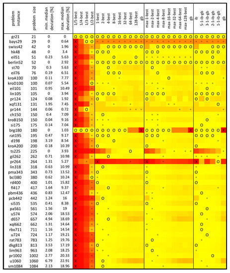
Figure 3.
Median results of MMAS without local optimization for TSP.
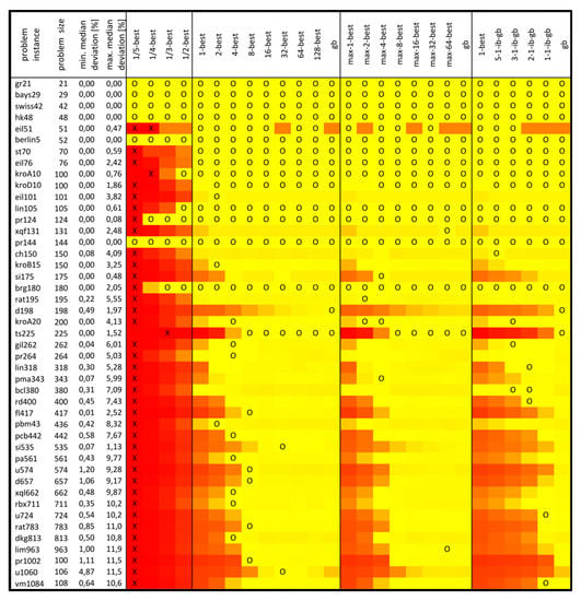
Figure 4.
Median results of MMAS with 2-opt local optimization for TSP.
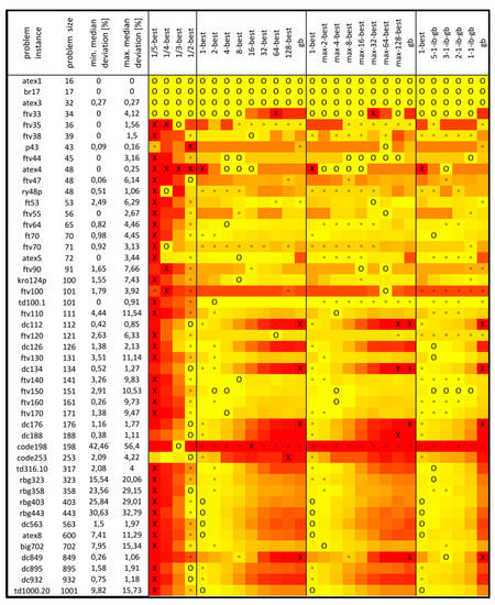
Figure 5.
Median results of MMAS without local optimization for ATSP.
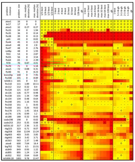
Figure 6.
Median results of MMAS witht 2.5-opt local optimization for ATSP.
For each problem instance, the best strategy was colored yellow, the worst strategy red, and all the other strategies with shades of colors in between. The best strategy is also marked with the symbol “O” and the worst with the symbol “X”. Strategies that were the best within their own category are marked by the symbol “°”. In some cases, there is more than one best strategy, e.g., MMAS without local optimization achieves a median solution equal to the optimum for gr21 for all strategies, as shown in Figure 3.
Since κ-best and max-κ-best are intended to be adjustable and extended with the 1/λ-best strategy, we also performed statistical analyses of combined strategies based on counting.
In addition, if, for some reason, it is not possible to adjust the appropriate strategy before the algorithm is used for solving some problem instance in practice, one possible approach would be to choose the strategy with the lowest average rank, as used in the Friedman test. Therefore, we also calculated the average rank for each strategy and performed the Friedman test and a post hoc procedure []. The null hypothesis of the Friedman test is that there is no difference in performance of MMAS algorithm for tested pheromone reinforcement strategies. If the P-value is lower than the significance level α, which is usually set to 0.05, then the null hypothesis is rejected. When the null hypothesis is rejected, this means that the difference in results for some strategies is not due to statistical error. However, this does not mean that each strategy provided a statistically significant difference in comparison to every other strategy. To statistically compare the strategy with the best average rank with every other strategy, pairwise comparisons can be performed in a post hoc procedure, for which we used Holm’s and Hochberg’s procedures [].
7.1. Results of the MAX-MIN Ant System without Local Optimization for TSP
Results of MMAS without local optimization, presented in Figure 3, show that choosing an appropriate strategy can make a significant difference in the performance of the algorithm. For some problem instances, the algorithm with the most suitable strategy was able to obtain a median solution equal to the optimum, while the most unsuitable strategy has a median solution that is a few percent worse than the optimum. This is, e.g., the case with hk48, lin105, brg180, ts225, and some others. There are also some cases where the most successful strategies have a median solution less than 1% worse than optimum, but unsuccessful strategies have a median solution more than 10% worse than optimum, such as in the cases of eil101, kroA200, lin318, pma343, pbm436, and some others. Thus, using an appropriate strategy is very important.
By looking at colors, it is obvious that most red-colored strategies are of the 1/λ-best type, while most “X” marks are on the 1/5-best strategy. There is also a certain similarity between the coloring of κ-best and max-κ-best and to some degree also to ib-gb scheduling. This shows that for some problem instances, the algorithm has similar behavior with respect to a similar level of gridlines.
To create an entire spectrum of adjustable strategies, we have proposed κ-best, max-κ-best, and 1/λ-best strategies. In that respect, it is important to evaluate their capabilities in contrast to classical iteration-best and global-best strategies and occasionally use ib-gb scheduling. By counting exclusive wins, it is noticeable that iteration best has 5 out of 45 (11%) exclusive wins, global best has 0, strategy 1/λ-best for λ = {5, 4, 3, 2} has 4 (9%), strategy κ-best for κ = {2, 4, 8, 16, 32, 64, 128} has 10 (22%), strategy max-κ-best for κ = {2, 4, 8, 16, 32, 64, 128} has 3 (7%), and ib-bg scheduling for combinations {5-1, 3-1, 2-1, 1-1} has 12 (27%) of exclusive wins.
When combined in some logical way so it could be adjusted by parametric number or schedule, the results of total wins (not exclusive wins) are summarized in Table 3. Any adjustable choice would be better than simply using ib or gb strategies, but 1/λ-best and κ-best seem most promising, followed by ib-gb scheduling with included ib and gb, and finally by 1/λ-best and max-κ-best.
Table 3.
The Number of Wins for Combined Strategies in the Case of MMAS for TSP without Local Optimization.
If for some reason, strategy is not adjusted to a particular problem instance, and normally it should be, then the best average rank strategy might be used; in this case, this is 3-1-ib-gb, followed by 5-1-ib-gb, 2-best, 4-best, max-2-best, max-4-best, etc., with average ranks 6.8222, 6.9444, 7.0556, 7.0778, 7.5889, and 7.7111, respectively. The worst average rank, 23.2889, was achieved by 1/5-best. Friedman statistic Q (distributed according to chi-square with 23 degrees of freedom) is 537.807778, which corresponds to p-value 4.67⋅10−99, while Iman and Davenport statistic T (distributed according to F-distribution with 23 and 1012 degrees of freedom) is 47.594353, which corresponds to p-value 1.9⋅10−143, so both p-values are much lower than the usual significance level 0.05. This means that differences in results obtained by different strategies are statistically significant.
In the post hoc analysis, we used Holm’s and Hochberg’s procedures to pairwise compare the strategy that has the best average rank (3-1-ib-gb) with all the other strategies. Both post hoc procedures, with an overall significance level of 0.05, could not reject the null hypotheses for 5-1-ib-gb, 2-best, 4-best, max-2-best, max-4-best, 2-1-ib-gb, 8-best, 1-best, 1-1-ib-gb, and max-8-best, but they rejected the null hypotheses for all other strategies.
7.2. Results of the MAX-MIN Ant System with 2-opt Local Optimization for TSP
Figure 4 contains the results observed by the MMAS with 2-opt local optimization that accepts the first improvement. These results show that using an appropriate strategy is important because with the most successful strategy, the algorithm achieved for almost all instances a median solution that is less than 1% distant from the optimum, but for an inappropriate strategy, this can be more than 10%. As was the case with MMAS for TSP without local optimization, most of the red area is within the 1/λ-strategy. There are also similarities between κ-best, max-κ-best, and ib-gb-scheduling, which might be interpreted as similar behavior of the algorithm for similar levels of a strategy’s greediness. In this case, it can be observed that for larger problem instances, the less greedy strategies cause poor performance.
When considering the number of exclusive wins by some strategies, 1/λ-best and iteration best have zero exclusive wins. The global best has only one exclusive win. The most exclusive wins have κ-best, 16 out of 45 (36%), followed by ib-gb scheduling, 6 out of 45 (13%), and max-κ-best, 5 out of 45 (11%).
In the case of combined strategies, as shown in Table 4, it is obvious that adjustable strategies can improve the algorithmic performance in comparison with the classical approach of using only iteration best and global best. In this case, the most successful strategy was κ-best, followed by ib-gb scheduling and max-κ-best.
Table 4.
The Number of Wins for Combined Strategies in the Case of MMAS for TSP with 2-opt Local Optimization.
If the strategy is not adjusted to a problem instance (adjusting is highly recommended), then the 8-best strategy might be used as a strategy that achieved the best average rank in this group of experiments. After the 8-best strategy (average rank = 8.4), the descending order follows max-4-best, max-8-best, 1-1-ib-gb, 4-best, 32-best, etc., with average ranks of 8.7, 8.9444, 9.1333, 9.3333, and 9.5333, respectively. The worst average rank, 22.3889, was achieved by 1/5-best. Friedman statistic Q is 377.231778, which corresponds to p-value 8.47⋅10−66, while Iman and Davenport statistic T is 25.234114, which corresponds to p-value 1.5⋅10−83, so both p-values are much lower than the usual significance level of 0.05.
In the post hoc analysis, Holm’s and Hochberg’s procedures compared with equal decisions: the 8-best strategy against all the other strategies. The null hypotheses could not be rejected for max-4-best, max-8-best, 1-1-ib-gb, 4-best, 32-best, 64-best, global best, 128-best, max-64-best, max-16-best, max-32-best, 16-best, max-128-best, 2-1-ib-gb, 3-1-ib-gb, or 2-best but was rejected for all other strategies.
7.3. Results of the MAX-MIN Ant System without Local Optimization for ATSP
The results of MMAS for ATSP are presented in Figure 5. With the most successful strategies, the algorithm for some instances achieved a median solution that is optimal, but for other instances, it was up to 42.6% worse than optimal. For some instances, choosing the appropriate strategy is more important with respect to distance from optimum, while for others, it is not that important. For most instances, the worst strategy was 1/λ-best, and generally, there is a similarity between κ-best, max-κ-best, and ib-gb scheduling strategies with respect to level of greediness and algorithmic performance.
When exclusive wins are counted, 1/λ-best with λ = {5, 4, 3, 2} has 13 out of 47 (28%), iteration best has 5 (11%), κ-best with κ = {2, 4, 8, 16, 32, 64, 128} has 8 (17%), max-κ-best also has 8 (17%), ib-gb scheduling has 6 (13%), and global best has 0 exclusive wins.
All dc* problem instances (dc112, dc126, …, dc932) have a similar pattern, where for 1/2-best and iteration best, the algorithm gave the best performance (only for d849, this is 8-best or max-8-best), and greedier k-best or max-k-best strategies have rather bad performance.
When counting all wins, as shown in Table 5, the largest number of wins has a combination of 1/λ-best and κ-best and a combination of 1/λ-best and max-κ-best, both 70.2%, followed by ib-gb scheduling, which includes ib and gb and has 38.3% wins.
Table 5.
The Number of Wins for Combined Strategies in the Case of MMAS for ATSP without Local Optimization.
When the strategies are not adjusted for a particular problem instance, the strategy with the best average rank, in this case 5-1-ib-gb, might be used. The strategies with the best ranks are 5-1-ib-gb (7.6489), 2-best (7.8085), 3-1-ib-gb (8.1596), max-2-best (8.6277), 4-best (8.9255), 2-1-ib-gb (9.0319), etc. The worst average rank, 21.0957, has the 1/5-best strategy. Friedman statistic Q = 334.488085, which corresponds with p-value = 4.62⋅10−57, while Iman and Davenport statistic T, distributed according to F-distribution with 23 and 1058 degrees of freedom, is 20.611127, which corresponds with p-value = 1.52⋅10−69, both much lower than 0.05.
In Holm’s and Hochberg’s post hoc procedures with 5-1-ib-gb against others, the null hypotheses could not be rejected against 2-best, 3-1-ib-gb, max-2-best, 4-best, 2-1-ib-gb, 1-best, 8-best, max-4-best, max-8-best, 1/2-best, or 1-1-ib-gb, but it was rejected for all other strategies.
7.4. Results of the MAX-MIN Ant System with 2.5-opt Local Optimization for ATSP
The results for ATSP obtained by MMAS with 2.5-opt local optimization are presented in Figure 6. For almost all but a few problem instances, with a suitable strategy, the algorithm obtained median solutions less than 1% within optimum and often completely equal to optimum. In the case when reinforcement strategy was not adequately matched with the characteristics of the problem instance, for some instances the median solutions were more than 10% worse than optimum. The distribution of red color is more complex and not so dominantly reserved for the 1/λ-strategy as with other tested algorithms. There are also obvious similarities between κ-best, max-κ-best, and ib-gb scheduling with respect to the level of greediness and corresponding algorithmic performance.
When it comes to exclusive wins, 1/λ-best with λ = {5, 4, 3, 2} has 11 out of 47 (23%), iteration best has 0, κ-best has 10 (21%), max-κ-best has 3 (6%), both with κ = {2, 4, 8, 16, 32, 64, 128}, ib-gb scheduling has 16 (34%), and global best has 0.
Table 6 presents summarized results for combinations that cover a wider range of numerically controlled strategies. The best in terms of all wins was combination 1/λ-best and κ-best, followed by ib-gb scheduling with included ib and gb, and 1/λ-best and max-κ-best. So, any of these combinations allowed better performance through adjustability than only using iteration-best and global-best strategies.
Table 6.
The Number of Wins for Combined Strategies in the Case of MMAS for ATSP with 2.5-opt Local Optimization.
In the cases of some instances, the lower level of greediness is preferred, but in others, it is the opposite. There are also some cases where only 1/5-best and 1/4-best strategies allow the best performance of the algorithm.
The strategies with the best average ranks are 3-1-ib-gb (8.4468), 5-1-ib-gb (8.7766), 2-1-ib-gb (8.8191), 1-1-ib-gb (9.734), 4-best (10.1489), max-2-best (10.4149), etc. The worst average rank, 18.5426, has the 1/5-best strategy. Friedman statistic Q = 148.90383, which corresponds with p-value = 2.04 × 10⁻²⁰, while Iman and Davenport statistic T, distributed according to F-distribution with 23 and 1058 degrees of freedom, is 7.348572, which corresponds with p-value = 3.45 × 10⁻²², both much lower than 0.05.
Holm’s post hoc procedure, as well as Hochberg’s procedure with the 3-1-ib-gb against others, could not reject the null hypotheses for 5-1-ib-gb, 2-1-ib-gb, 1-1-ib-gb, 4-best, max-2-best, 2-best, 8-best, 1-best, 16-best, max-4-best, max-8-best, or 1/2-best, but it was rejected for all other strategies.
8. Discussion
A large number of experiments were carried out in this research to allow the analysis of the behavior of ant colony optimization algorithms (MMASs with and without local optimization) with respect to different pheromone trail reinforcement strategies that can be adjusted with numerical parameters. The experiments confirmed that, by using numerically adjustable strategies, it is possible to significantly improve algorithmic performance. Although some regularities between different strategies were observed, they are not so clear and simple as to would allow the recommending of some predefined parameters and strategy that would be the best for all problem instances and all variants of the algorithms. There is also a similarity between κ-best, max-κ-best, and ib-gb scheduling, so it is possible to fine tune an algorithm by using only one of these strategies, although in some cases κ-best and max-κ-best should be extended with 1/λ-best to one compound numerically controlled strategy with a lower level of greediness.
In our previous studies, we had some limited experiences with new adjustable strategies that helped us, in some cases, achieve the state-of-the-art results. However, there were no comprehensive analyses that would allow us to estimate the potential of adjustable strategies as a tool for improving ACO algorithms. The introduction of 1/λ-best was motivated by our observation that in the case of the quadratic assignment problem, which does not use heuristic information and, thus, has much higher exploration at the start, often strategies with low greediness provide the best results. Because of this, we wanted to further extend numerically adjustable strategies in a way that they could be even less greedy than iteration best. To our surprise, this research showed that 1/λ-best can have some success even with TSP, which, however, has very efficient heuristic information. For MMAS without local optimization, 1/λ-best had some occasions of great success in contrast to a classically used global-best strategy that had 0 exclusive wins, but in most cases, global best is safer for scenarios where there is limited parameter tuning. The 1/λ-best is recommended only in combination, preferably with 1/λ-best or alternatively with max-κ-best. The 1/λ-best was shown to be rather important for ATSP with and even more without local optimization. Only in the case of TSP, for which the MMAS with good local optimization (2-opt) allows faster coverage toward very good solutions, implementing the 1/λ-best strategy seems completely unnecessary.
Judging by the results of these experiments, it seems that the higher level of greediness is better for TSP with larger problem instances, especially when local optimization is used, but for ATSP, the level of desirable greediness seems to be more connected to a group of problem instances, presuming with similar structure, than it was with the size of the problem. So, in the case of problems with good heuristic information, it might be helpful to implement 1/λ-best and k-best strategies and try κ-best first. If lower values for κ give better results, then smaller λ parameters might also be worth trying.
When considering the good potential of numerically adjustable strategies, it could be worth trying them all for problems that are related to TSP and ATSP and have efficient heuristic information like SOP, VRPs, CaRS, CaRSP, etc.
It is a highly advisable to adjust the pheromone reinforcement strategy to a particular problem instance that should be solved, but if, for some reason, this is not possible, then the strategy with the best average rank with similar problem instance and working conditions might be used. We used Friedman test with Holm’s and Hochberg’s procedures to test the statistical significance of differences among achieved average ranks.
In our future research, in addition to trying out adjustable strategies for some of the aforementioned problems, we plan to carry out a comprehensive study with ACO for a combinatorial problem that does not have useful heuristic information and presumably might find a strategy with a low level of greediness a good fit for overall balancing between exploration and exploitation.
Author Contributions
Conceptualization, N.I.; methodology, N.I., R.K. and M.G.; software, N.I.; validation, N.I., R.K. and M.G.; formal analysis, N.I.; investigation, N.I. and R.K.; resources, N.I. and M.G.; data curation, N.I.; writing—original draft preparation, N.I. and R.K.; writing—review and editing, N.I.; visualization, N.I.; supervision, M.G.; project administration, N.I. and M.G.; funding acquisition, N.I., R.K. and M.G. All authors have read and agreed to the published version of the manuscript.
Funding
This work has been supported by the Croatian Science Foundation under the Project IP-2019-04-4864.
Data Availability Statement
In this research, we used publicly available problem instances from http://comopt.ifi.uni-heidelberg.de/software/TSPLIB95/, accessed on 1 April 2023, https://www.math.uwaterloo.ca/tsp/vlsi/, accessed on 1 April 2023, and http://dimacs.rutgers.edu/, accessed on 1 April 2023.
Acknowledgments
Computational resources provided by the Isabella cluster (isabella.srce.hr) at Zagreb University Computing Centre (SRCE) were used to conduct the experimental research described in this publication.
Conflicts of Interest
The authors declare no conflict of interest.
References
- Leguizamón, G.; Coello, C.A.C. An alternative ACOR algorithm for continuous optimization problems. In Proceedings of the 7th International Conference on Swarm Intelligence, ANTS’10, Brussels, Belgium, 8–10 September 2010; Springer: Berlin/Heidelberg, Germany, 2010; pp. 48–59. [Google Scholar]
- Liao, T.; Socha, K.; Montes de Oca, M.A.; Stützle, T.; Dorigo, M. Ant Colony Optimization for Mixed-Variable Optimization Problems. IEEE Trans. Evol. Comput. 2014, 18, 503–518. [Google Scholar] [CrossRef]
- Liu, J.; Anavatti, S.; Garratt, M.; Abbass, H.A. Modified continuous Ant Colony Optimisation for multiple Unmanned Ground Vehicle path planning. Expert Syst. Appl. 2022, 196, 116605. [Google Scholar] [CrossRef]
- Liao, T.W.; Kuo, R.; Hu, J. Hybrid ant colony optimization algorithms for mixed discrete–continuous optimization problems. Appl. Math. Comput. 2012, 219, 3241–3252. [Google Scholar] [CrossRef]
- Omran, M.G.; Al-Sharhan, S. Improved continuous Ant Colony Optimization algorithms for real-world engineering optimization problems. Eng. Appl. Artif. Intell. 2019, 85, 818–829. [Google Scholar] [CrossRef]
- Chen, Z.; Zhou, S.; Luo, J. A robust ant colony optimization for continuous functions. Expert Syst. Appl. 2017, 81, 309–320. [Google Scholar] [CrossRef]
- Kudelić, R.; Ivković, N. Ant inspired Monte Carlo algorithm for minimum feedback arc set. Expert Syst. Appl. 2019, 122, 108–117. [Google Scholar] [CrossRef]
- Stützle, T.; Hoos, H.H. MAX-MIN Ant System. Future Gener. Comput. Syst. 2000, 16, 889–914. [Google Scholar] [CrossRef]
- Gambardella, L.M.; Montemanni, R.; Weyland, D. An Enhanced Ant Colony System for the Sequential Ordering Problem. In Operations Research Proceedings 2011, Proceedings of the International Conference on Operations Research (OR 2011), Zurich, Switzerland, 30 August–2 September 2011; Klatte, D., Lüthi, H.J., Schmedders, K., Eds.; Springer: Berlin/Heidelberg, Germany, 2012; pp. 355–360. [Google Scholar]
- Skinderowicz, R. An improved Ant Colony System for the Sequential Ordering Problem. Comput. Oper. Res. 2017, 86, 1–17. [Google Scholar] [CrossRef]
- Ky Phuc, P.N.; Phuong Thao, N.L. Ant Colony Optimization for Multiple Pickup and Multiple Delivery Vehicle Routing Problem with Time Window and Heterogeneous Fleets. Logistics 2021, 5, 28. [Google Scholar] [CrossRef]
- Jia, Y.H.; Mei, Y.; Zhang, M. A Bilevel Ant Colony Optimization Algorithm for Capacitated Electric Vehicle Routing Problem. IEEE Trans. Cybern. 2022, 52, 10855–10868. [Google Scholar] [CrossRef]
- Popović, E.; Ivković, N.; Črepinšek, M. ACOCaRS: Ant Colony Optimization Algorithm for Traveling Car Renter Problem. In Bioinspired Optimization Methods and Their Applications; Mernik, M., Eftimov, T., Črepinšek, M., Eds.; Springer International Publishing: Cham, Switzerland, 2022; pp. 31–45. [Google Scholar]
- Ivkovic, N.; Malekovic, M.; Golub, M. Extended Trail Reinforcement Strategies for Ant Colony Optimization. In Swarm, Evolutionary, and Memetic Computing, Proceedings of the Second International Conference, SEMCCO 2011, Visakhapatnam, India, 19–21 December 2011; Lecture Notes in Computer Science; Panigrahi, B.K., Suganthan, P.N., Das, S., Satapathy, S.C., Eds.; Springer: Berlin/Heidelberg, Germany, 2011; Volume 7076, pp. 662–669. [Google Scholar] [CrossRef]
- Dorigo, M.; Maniezzo, V.; Colorni, A. Positive Feedback as a Search Strategy; Technical Report 91-016; Dipartimento di Elettronica, Politecnico di Milano: Milano, Italy, 1991. [Google Scholar]
- Dorigo, M.; Maniezzo, V.; Colorni, A. Ant system: Optimization by a colony of cooperating agents. IEEE Trans. Syst. Man Cybern. Part B 1996, 26, 29–41. [Google Scholar] [CrossRef] [PubMed]
- Dorigo, M.; Gambardella, L.M. Ant colony system: A cooperative learning approach to the traveling salesman problem. IEEE Trans. Evol. Comput. 1997, 1, 53–66. [Google Scholar] [CrossRef]
- Dorigo, M. Optimization, Learning and Natural Algorithms. Ph.D. Thesis, Politecnico di Milano, Milano, Italy, 1992. (In Italian). [Google Scholar]
- Bullnheimer, B.; Hartl, R.F.; Strauss, C. A New Rank Based Version of the Ant System: A Computational Study. Cent. Eur. J. Oper. Res. Econ. 1999, 7, 25–38. [Google Scholar]
- Cordón, O.; de Viana, I.F.; Herrera, F. Analysis of the Best-Worst Ant System and Its Variants on the QAP. In Ant Algorithms, Proceedings of the Third International Workshop, ANTS 2002, Brussels, Belgium, 12–14 September 2002; Springer: Berlin/Heidelberg, Germany, 2002; pp. 228–234. [Google Scholar]
- Cordón, O.; de Viana, I.F.; Herrera, F. Analysis of the Best-Worst Ant System and its Variants on the TSP. Mathw. Soft Comput. 2002, 9, 177–192. [Google Scholar]
- Guntsch, M.; Middendorf, M. Applying Population Based ACO to Dynamic Optimization Problems. In Ant Algorithms, Proceedings of the Third International Workshop, ANTS 2002, Brussels, Belgium, 12–14 September 2002; Springer: Berlin/Heidelberg, Germany, 2002; pp. 111–122. [Google Scholar]
- Guntsch, M.; Middendorf, M. A Population Based Approach for ACO. In Applications of Evolutionary Computing, Proceedings of the EvoWorkshops 2002: EvoCOP, EvoIASP, EvoSTIM/EvoPLAN, Kinsale, Ireland, 3–4 April 2002; Lecture Notes in Computer Science; Cagnoni, S., Gottlieb, J., Hart, E., Middendorf, M., Raidl, G.R., Eds.; Springer: Berlin/Heidelberg, Germany, 2002; Volume 2279, pp. 72–81. [Google Scholar]
- Deng, X.; Zhang, L.; Lin, H.; Luo, L. Pheromone mark ant colony optimization with a hybrid node-based pheromone update strategy. Neurocomputing 2015, 148, 46–53. [Google Scholar] [CrossRef]
- Guntsch, M.; Middendorf, M. Pheromone Modification Strategies for Ant Algorithms Applied to Dynamic TSP. In Applications of Evolutionary Computing, Proceedings of the EvoWorkshops 2001: EvoCOP, EvoFlight, EvoIASP, EvoLearn, and EvoSTIM, Como, Italy, 18–20 April 2001; Lecture Notes in Computer Science; Boers, E.J.W., Gottlieb, J., Lanzi, P.L., Smith, R.E., Cagnoni, S., Hart, E., Raidl, G.R., Tijink, H., Eds.; Springer: Berlin/Heidelberg, Germany, 2001; Volume 2037, pp. 213–222. [Google Scholar]
- Wang, L.; Shen, J.; Luo, J. Impacts of Pheromone Modification Strategies in Ant Colony for Data-Intensive Service Provision. In Proceedings of the 2014 IEEE International Conference on Web Services, ICWS, Anchorage, AK, USA, 27 June–2 July 2014; IEEE Computer Society: Washington, DC, USA, 2014; pp. 177–184. [Google Scholar]
- Liu, G.; He, D. An improved Ant Colony Algorithm based on dynamic weight of pheromone updating. In Proceedings of the Ninth International Conference on Natural Computation, ICNC 2013, Shenyang, China, 23–25 July 2013; Wang, H., Yuen, S.Y., Wang, L., Shao, L., Wang, X., Eds.; IEEE: Piscataway, NJ, USA, 2013; pp. 496–500. [Google Scholar] [CrossRef]
- Lalbakhsh, P.; Zaeri, B.; Lalbakhsh, A. An Improved Model of Ant Colony Optimization Using a Novel Pheromone Update Strategy. IEICE Trans. Inf. Syst. 2013, E96.D, 2309–2318. [Google Scholar] [CrossRef]
- Bacanin, N.; Stoean, R.; Zivkovic, M.; Petrovic, A.; Rashid, T.A.; Bezdan, T. Performance of a Novel Chaotic Firefly Algorithm with Enhanced Exploration for Tackling Global Optimization Problems: Application for Dropout Regularization. Mathematics 2021, 9, 2705. [Google Scholar] [CrossRef]
- Malakar, S.; Ghosh, M.; Bhowmik, S.; Sarkar, R.; Nasipuri, M. A GA based hierarchical feature selection approach for handwritten word recognition. Neural Comput. Appl. 2019, 32, 2533–2552. [Google Scholar] [CrossRef]
- Michel, R.; Middendorf, M. An Island Model Based Ant System with Lookahead for the Shortest Supersequence Problem. In Proceedings of the 5th International Conference on Parallel Problem Solving from Nature—PPSN V, Amsterdam, The Netherlands, 27–30 September 1998; Springer: Berlin/Heidelberg, Germany, 1998; pp. 692–701. [Google Scholar]
- Solnon, C.; Fenet, S. A study of ACO capabilities for solving the maximum clique problem. J. Heuristics 2006, 12, 155–180. [Google Scholar] [CrossRef]
- Gambardella, L.M.; Taillard, E.; Agazzi, G. MACS-VRPTW: A Multiple Ant Colony System for Vehicle Routing Problems with Time Windows. In New Ideas in Optimization; McGraw-Hill Ltd.: London, UK, 1999; pp. 63–76. [Google Scholar]
- Ivković, N. Modeling, Analysis and Improvement of Ant Colony Optimization Algorithms. Ph.D. Thesis, University of Zagreb, Zagreb, Croatia, 2014. (In Croatian). [Google Scholar]
- Ivković, N.; Golub, M. A New Ant Colony Optimization Algorithm: Three Bound Ant System. In Swarm Intelligence, Proceedings of the 9th International Conference, ANTS 2014, Brussels, Belgium, 10–12 September 2014; Lecture Notes in Computer Science; Dorigo, M., Birattari, M., Garnier, S., Hamann, H., de Oca, M.A.M., Solnon, C., Stützle, T., Eds.; Springer: Berlin/Heidelberg, Germany, 2014; Volume 8667, pp. 280–281. [Google Scholar]
- Ivković, N. Ant Colony Algorithms for the Travelling Salesman Problem and the Quadratic Assignment Problem. In Swarm Intelligence—Volume 1: Principles, Current Algorithms and Methods; The Institution of Engineering and Technology: London, UK, 2018; pp. 409–442. [Google Scholar]
- Dorigo, M.; Stützle, T. Ant Colony Optimization; The MIT Press: Cambridge, MA, USA, 2004. [Google Scholar] [CrossRef]
- Ivkovic, N.; Jakobovic, D.; Golub, M. Measuring Performance of Optimization Algorithms in Evolutionary Computation. Int. J. Mach. Learn. Comput. 2016, 6, 167–171. [Google Scholar] [CrossRef]
- Ivković, N.; Kudelić, R.; Črepinšek, M. Probability and Certainty in the Performance of Evolutionary and Swarm Optimization Algorithms. Mathematics 2022, 10, 4364. [Google Scholar] [CrossRef]
- Derrac, J.; García, S.; Molina, D.; Herrera, F. A practical tutorial on the use of nonparametric statistical tests as a methodology for comparing evolutionary and swarm intelligence algorithms. Swarm Evol. Comput. 2011, 1, 3–18. [Google Scholar] [CrossRef]
Disclaimer/Publisher’s Note: The statements, opinions and data contained in all publications are solely those of the individual author(s) and contributor(s) and not of MDPI and/or the editor(s). MDPI and/or the editor(s) disclaim responsibility for any injury to people or property resulting from any ideas, methods, instructions or products referred to in the content. |
© 2023 by the authors. Licensee MDPI, Basel, Switzerland. This article is an open access article distributed under the terms and conditions of the Creative Commons Attribution (CC BY) license (https://creativecommons.org/licenses/by/4.0/).