Smooth Information Criterion for Regularized Estimation of Item Response Models

Abstract

Item response theory (IRT) models are frequently used to analyze multivariate categorical data from questionnaires or cognitive test data. In order to reduce the model complexity in item response models, regularized estimation is now widely applied, adding a nondifferentiable penalty function like the LASSO or the SCAD penalty to the log-likelihood function in the optimization function. In most applications, regularized estimation repeatedly estimates the IRT model on a grid of regularization parameters $\mathsf{\lambda }$. The final model is selected for the parameter that minimizes the Akaike or Bayesian information criterion (AIC or BIC). In recent work, it has been proposed to directly minimize a smooth approximation of the AIC or the BIC for regularized estimation. This approach circumvents the repeated estimation of the IRT model. To this end, the computation time is substantially reduced. The adequacy of the new approach is demonstrated by three simulation studies focusing on regularized estimation for IRT models with differential item functioning, multidimensional IRT models with cross-loadings, and the mixed Rasch/two-parameter logistic IRT model. It was found from the simulation studies that the computationally less demanding direct optimization based on the smooth variants of AIC and BIC had comparable or improved performance compared to the ordinarily employed repeated regularized estimation based on AIC or BIC.

1. Introduction

Item response theory (IRT; [1,2,3,4,5]) modeling is a class of statistical models that analyze discrete multivariate data. In these models, a vector $\mathit{X}=(X_1,\dots ,X_I)$ of I discrete variables $X_i$ ($i=1,\dots ,I$; also referred to as items) is summarized by a unidimensional or multidimensional factor variable $\mathsf{\theta }$. In this article, we confine ourselves to dichotomous random variables $X_i\in \{0,1\}$.

The multivariate distribution for the vector $\mathit{X}\in {\{0,1\}}^I$ in the IRT model is defined as

$$\mathsf{P}(\mathit{X}=\mathit{x};\gamma )=\int \prod _{i=1}^I\mathsf{P}(X_i=x_i|\mathsf{\theta };{\gamma }_i)f(\mathsf{\theta };\mathsf{\beta })\mathrm{d}\mathsf{\theta },$$

(1)

where $\gamma =({\gamma }_1,\dots ,{\gamma }_I,\mathsf{\beta })$ is the vector of model parameters. The vector ${\gamma }_i$ contains item parameters of item i, while $\mathsf{\beta }$ parametrizes the density f of the factor variable $\mathsf{\theta }$. Note that (1) includes a local independence assumption. That is, the items $X_i$ are conditionally independent given the factor variable $\mathsf{\theta }$. The function $\mathsf{\theta }\mapsto \mathsf{P}(X_i=x_i|\mathsf{\theta };{\gamma }_i)$ is also referred to as the item response function (IRF; [6,7,8]). The two-parameter logistic (2PL) model [9] uses the IRF $\mathsf{\theta }\mapsto \mathsf{\Psi }(a_i\mathsf{\theta }-b_i)$, where $\mathsf{\Psi }$ denotes the logistic distribution function.

Now, assume that N independent replications of $\mathit{X}$ are available. The parameter vector $\gamma$ from these observations ${\mathit{x}}_1,\dots ,{\mathit{x}}_N$ can be estimated by minimizing the negative log-likelihood function

$$l\left(\gamma \right)=-\sum _{n=1}^{N}log\mathsf{P}(\mathit{X}={\mathit{x}}_n;\gamma ),$$

(2)

where the parameter vector $\gamma =({\gamma }_1,\dots ,{\gamma }_H)$ contains H components that have to be estimated.

In various applications, the IRT model (1) is not identified or includes too many parameters, making the interpretation difficult. To this end, some sparsity structure [10] on model parameters $\gamma$ is imposed. Regularized estimation as a machine learning technique is employed in IRT models to make estimation feasible [11,12,13]. More formally, sparsity structure on $\gamma$ is imposed by replacing the negative log-likelihood function with a negative regularized log-likelihood function

$$l_{\mathrm{reg}}(\gamma ;\mathsf{\lambda })=l\left(\gamma \right)+N\sum _{h=1}^H{\mathsf{\iota }}_h\mathcal{P}({\gamma }_h,\mathsf{\lambda }),$$

(3)

where ${\iota }_h$ is an indicator variable for the parameter ${\gamma }_h$ that takes values 0 or 1. The indicator ${\iota }_h$ equals 1 if ${\gamma }_h$ is regularized (i.e., the sparsity structure assumption applies to this parameter), while it is 0 if ${\gamma }_h$ should not be regularized. Let $H_1={\sum }_{h=1}^H{\iota }_h$ be the number of regularized parameters and $H_0=H-H_1$ is the number of nonregularized model parameters. The regularized negative log-likelihood function $l_{\mathrm{reg}}$ defined in (3) includes a penalty function $\mathcal{P}$ that decodes the assumptions about sparsity. For a scalar parameter x, the least absolute shrinkage and selection operator (LASSO; [14]) penalty is a popular penalty function used in regularization, and it is defined as

$${\mathcal{P}}_{\mathrm{LASSO}}(x,\mathsf{\lambda })=\mathsf{\lambda }\left|x\right|,$$

(4)

where $\mathsf{\lambda }$ is a nonnegative regularization parameter that controls the extent of sparsity in the obtained parameter estimate. It is well-known that the LASSO penalty introduces bias in estimated parameters. To circumvent this issue, the smoothly clipped absolute deviation (SCAD; [15]) penalty has been proposed.

$${\mathcal{P}}_{\mathrm{SCAD}}(x,\mathsf{\lambda })=\left\{\begin{array}{cc}\mathsf{\lambda }\left|x\right|\hfill & \mathrm{if}\left|x\right|<\mathsf{\lambda }\hfill \\ -(x^2-{2a\mathsf{\lambda }\left|x\right|}^2+{\mathsf{\lambda }}^2{)\left(2(a-1)\right)}^{-1}\hfill & \mathrm{if}\mathsf{\lambda }\le \left|x\right|\le a\mathsf{\lambda }\hfill \\ (a+1){\mathsf{\lambda }}^2\hfill & \mathrm{if}\left|x\right|>a\mathsf{\lambda }\hfill \end{array}\right.$$

(5)

In many studies, the recommended value of $a=3.7$ (see [15]) has been adopted (e.g., [10,16]). Note that ${\mathcal{P}}_{\mathrm{SCAD}}$ has the property of the LASSO penalty around zero, but has zero derivatives for x values that strongly differ from zero.

A parameter estimate $\widehat{\gamma }$ of the regularized IRT model is defined as an estimator defined as the minimizer of $l_{\mathrm{reg}}$

$$\widehat{\gamma }\left(\mathsf{\lambda }\right)=\underset{\gamma }{arg\; min}{l}_{\mathrm{reg}}(\gamma ;\mathsf{\lambda }).$$

(6)

Note that the penalty function $\mathcal{P}$ involves a fixed tuning parameter $\mathsf{\lambda }$. Hence, the parameter estimate $\widehat{\gamma }\left(\mathsf{\lambda }\right)$ depends on $\mathsf{\lambda }$. A crucial issue of the LASSO and the SCAD penalty functions is that they are nondifferentiable functions because the function $x\mapsto \left|x\right|$ is nondifferentiable. Hence, particular estimation techniques for nondifferentiable optimization problems must be applied [14,17,18]. As an alternative, the nondifferentiable optimization function can be replaced by a differentiable approximation [19,20,21,22]. For example, the absolute value function $x\mapsto \left|x\right|$ in the SCAD penalty can be replaced with $x\mapsto \sqrt{x^2+\mathsf{\epsilon }}$ for a sufficiently small $\mathsf{\epsilon }$ such as $\mathsf{\epsilon }=0.001$. Using differentiable approximations has the advantage that ordinary gradient-based optimizers can be utilized.

In practice, the estimation of the regularized IRT model is carried out on a grid of T values of $\mathsf{\lambda }$ in a grid $\mathsf{\Lambda }=\{{\mathsf{\lambda }}_1,\dots ,{\mathsf{\lambda }}_T\}$. For each value of the tuning parameter ${\mathsf{\lambda }}_t$, a parameter estimate $\widehat{\gamma }\left({\mathsf{\lambda }}_t\right)$ is obtained. A final parameter estimate $\widehat{\gamma }$ is obtained by minimizing an information criterion

$$IC\left(\widehat{\gamma }\left(\mathsf{\lambda }\right)\right)=2l\left(\widehat{\gamma }\left(\mathsf{\lambda }\right)\right)+K_N\left(H_0+\sum _{h=1}^H{\mathsf{\iota }}_h\mathbf{1}({\widehat{\gamma }}_h\left(\mathsf{\lambda }\right)\ne 0)\right),$$

(7)

where the factor $K_N$ is chosen as $K_N=2$ for the Akaike information criterion (AIC; [23]) and $K_N=logN$ for the Bayesian information criterion (BIC; [24]) (see [25]).

If the regularized likelihood function is evaluated with differentiable approximations, there are no regularized parameters that exactly equal zero (in contrast to special-purpose optimizers for regularized estimation; [17]). Hence, estimated parameters ${\gamma }_h$ are counted as zero if they do not exceed a fixed threshold $\tau$ (such as 0.001, 0.01, or 0.02) in its absolute value. Hence, the approximated information criterion is computed as

$$IC\left(\widehat{\gamma }\left(\mathsf{\lambda }\right)\right)=2l\left(\widehat{\gamma }\left(\mathsf{\lambda }\right)\right)+K_N\left(H_0+\sum _{h=1}^H{\mathsf{\iota }}_h\mathbf{1}\left(\right|{\widehat{\gamma }}_h\left(\mathsf{\lambda }\right)|>\mathsf{\tau })\right).$$

(8)

The final estimator of $\gamma$ is defined as

$${\widehat{\gamma }}_{IC}=\widehat{\gamma }\left({\widehat{\mathsf{\lambda }}}_{\mathrm{opt}}\right)\mathrm{with}{\widehat{\mathsf{\lambda }}}_{\mathrm{opt}}=\underset{\mathsf{\lambda }\in \mathsf{\Lambda }}{arg\; min}IC\left(\widehat{\gamma }\left(\mathsf{\lambda }\right)\right).$$

(9)

Depending on the chosen value of $K_N$, the regularized parameter estimate can be based on the AIC and BIC.

The ordinary estimation approach to regularized estimation described above has the computational disadvantage that it requires a sequential fitting of models on the grid $\mathsf{\Lambda }$ of the regularization parameter $\mathsf{\lambda }$. This approach is referred to as an indirect optimization approach because it first minimizes a criterion function (i.e., the regularized likelihood function) with respect to $\gamma$ for a fixed value of $\mathsf{\lambda }$ and optimizes a second criterion (i.e., the AIC or BIC) in the second step. O’Neill and Burke [26] proposed an estimation approach to regularized estimation that directly minimizes a smooth version of the BIC (i.e., smooth Bayesian information criterion, SBIC) for regression models. This direct estimation approach has been successfully implemented for structural equation models [21,27]. For these models, the optimization based on SBIC had similar, if not better, performance than the ordinary estimation of regularized models based on the AIC and BIC. In this paper, we explore whether the smooth information criteria SBIC and the smooth Akaike information criterion (SAIC) also hold promise for various applications in IRT models. Using a computationally cheaper alternative for regularized estimation is probably even more important for IRT models than for structural equation models because IRT models are more difficult to estimate and more computationally demanding. To the best of our knowledge, this is the first attempt at using smoothed information criteria in IRT models.

The rest of this paper is structured as follows. The optimization using smooth information criteria is outlined in Section 2. Afterward, three applications of regularized IRT models are investigated in three simulation studies. Section 3 presents Simulation Study 1, which studies regularized estimation for differential item functioning. Section 4 presents Simulation Study 2, which investigates the regularized estimation of multidimensional IRT models. The last Simulation Study 3 in Section 5 is devoted to regularized estimation of the mixed Rasch/2PL model. Finally, this study closes with a discussion in Section 6.

2. Smooth Information Criterion

In theory, a parameter estimate $\widehat{\gamma }$ for $\gamma$ of the IRT model may be obtained by directly minimizing an information criterion

$$\widehat{\gamma }=\underset{\gamma }{arg\; min}\left\{2l\left(\gamma \right)+K_N\left(H_0+\sum _{h=1}^H{\mathsf{\iota }}_h\mathbf{1}({\gamma }_h\ne 0)\right)\right\}.$$

(10)

The optimization function in (10) can be interpreted as a regularized log-likelihood function with an $L_0$ penalty [28,29]. Obviously, the indicator function $\mathbf{1}$ in (10) counts the number of regularized parameters that differ from zero. Researchers O’Neill and Burke [26] proposed substituting the indicator function with a suitable differentiable approximation ${\mathcal{N}}_{\mathsf{\epsilon }}$. To this end, a smooth information criterion, such as the SAIC and the SBIC, is obtained. In more detail, the differentiable approximation ${\mathcal{N}}_{\mathsf{\epsilon }}$ for $\mathbf{1}$ is defined as

$${\mathcal{N}}_{\mathsf{\epsilon }}\left(x\right)=\frac{x^2}{x^2+\mathsf{\epsilon }},$$

(11)

where $\mathsf{\epsilon }>0$ is a sufficiently small tuning parameter, such as $\mathsf{\epsilon }=0.001$. The function ${\mathcal{N}}_{\mathsf{\epsilon }}$ takes values close to zero for x arguments close to 0 and approaches 1 if $\left|x\right|$ moves away from 0. A smoothed information criterion $SIC\left(\gamma \right)$ (abbreviated as SIC) can be defined as

$$SIC\left(\gamma \right)=2l\left(\gamma \right)+K_N\left(H_0+\sum _{h=1}^H{\mathsf{\iota }}_h{\mathcal{N}}_{\mathsf{\epsilon }}\left({\gamma }_h\right)\right).$$

(12)

We obtain the SAIC for the choices of $K_N$ in (12) of $K_N=2$ and the SBIC for $K_N=log\left(N\right)$.

Hence, the minimization problem (10) can be replaced by

$$\widehat{\gamma }=\underset{\gamma }{arg\; min}SIC\left(\gamma \right)=\underset{\gamma }{arg\; min}\left\{2l\left(\gamma \right)+K_N\left(H_0+\sum _{h=1}^H{\mathsf{\iota }}_h{\mathcal{N}}_{\mathsf{\epsilon }}\left({\gamma }_h\right)\right)\right\}.$$

(13)

The optimization function in (13) directly minimizes a smoothed version of the information criterion.

3. Simulation Study 1: Differential Item Functioning

In the first Simulation Study 1, the assessment of differential item functioning (DIF; [30,31,32]) is considered as an example. DIF occurs in datasets with multiple groups if item parameters are not invariant (i.e., they are not equal) across groups. In this study, the case of two groups in the unidimensional 2PL model is treated. The IRF is given by

$$\mathsf{P}(X_i=1|G=g,\mathsf{\theta })=\mathsf{\Psi }\left(a_i\mathsf{\theta }-b_i-{\mathsf{\delta }}_i\mathbf{1}(G=2)\right)\mathrm{for}g=1,2,$$

(14)

where ${\mathsf{\delta }}_i$ indicates the DIF in item intercepts, which is also referred to as uniform DIF. The item parameters of item $X_i$ are given by ${\gamma }_i=(a_i,b_i,{\mathsf{\delta }}_i)$. The mean and the standard deviation of $\mathsf{\theta }$ in the first group are fixed for identification reasons to 0 and 1, respectively. Then, the mean ${\mathsf{\mu }}_2$ and the standard deviation ${\mathsf{\sigma }}_2$ of $\mathsf{\theta }$ in the second group can be estimated.

It has been pointed out that additional assumptions about DIF effects ${\mathsf{\delta }}_i$ must be imposed for model identification [33,34,35]. Assuming a sparsity structure on the DIF effects may be one plausible option. To this end, DIF effects ${\mathsf{\delta }}_i$ ($i=1,\dots ,I$) are regularized in the optimization based on the regularized log-likelihood function (3) or the minimization of the SIC (13). Regularized estimation of DIF in IRT models has been widely discussed in the literature [36,37,38,39,40,41,42].

3.1. Method

In this simulation study, we use a data-generating model (DGM) similar to the one used in the simulation study in [38]. The factor variable $\mathsf{\theta }$ was assumed to be univariate normally distributed. We fixed the mean ${\mathsf{\mu }}_1$ and the standard deviation ${\mathsf{\sigma }}_1$ of the factor variable $\mathsf{\theta }$ in the first group to 0 and 1, respectively. The factor variable $\mathsf{\theta }$ had a mean ${\mathsf{\mu }}_2$ of 0.5 and a standard deviation ${\mathsf{\sigma }}_2$ of 0.8 in the second group. In total, $I=25$ items were used in this simulation study.

We now describe the item parameters used for the IRF defined in (14). The common item discriminations $a_i$ of the 25 items were chosen as 1.3, 1.4, 1.5, 1.7, 1.6, 1.3, 1.4, 1.5, 1.7, 1.6, 1.3, 1.4, 1.5, 1.7, 1.6, 1.3, 1.4, 1.5, 1.7, 1.6, 1.3, 1.4, 1.5, 1.7, and 1.6. The item difficulties $b_i$ were chosen as −0.8, 0.4, 1.2, 2.0, −2.0, −0.8, 0.4, 1.2, 2.0, −2.0, −0.8, 0.4, 1.2, 2.0, −2.0, −0.8, 0.4, 1.2, 2.0, −2.0, −0.8, 0.4, 1.2, 2.0, and −2.0. The DIF effects ${\mathsf{\delta }}_i$ were zero for the first 15 items. Items 16 to 25 had non-zero DIF effects.

In the condition of small DIF effects (see [38]), we chose ${\mathsf{\delta }}_i$ values of −0.60, 0.60, −0.65, 0.70, 0.65, −0.70, 0.60, −0.65, 0.70, and −0.65 for Items 16 to 25. In the condition of large DIF effects, we multiplied these effects by 2. These two conditions are referred to as balanced DIF conditions because the DIF effects ${\mathsf{\delta }}_i$ average to zero. In line with other studies, we also considered unbalanced DIF [43], in which we took absolute DIF effects in the small DIF and large DIF conditions. In the unbalanced DIF conditions, all DIF effects ${\mathsf{\delta }}_i$ were assumed positive and did not average to zero. The item parameters can also be found at https://osf.io/ykew6 (accessed on 2 April 2024).

Moreover, we varied the sample size N in this simulation study by 500, 1000, and 2000. There were $N/2$ subjects in each of the two groups.

The regularized 2PL model with DIF was estimated with the regularized likelihood function using the SCAD penalty on a nonequidistant grid of 37 $\mathsf{\lambda }$ values between 0.0001 and 1 (see the R simulation code at https://osf.io/ykew6; accessed on 2 April 2024). We approximated the nondifferentiable SCAD penalty function by its differentiable approximating function using the tuning $\mathsf{\epsilon }=0.001$. We saved parameter estimates that minimized AIC and BIC. Item parameters that did not exceed the threshold $\tau =0.02$ in its absolute value were regularized. In the direct minimization of SAIC and SBIC, we tried the values 0.01, 0.001, and 0.0001 of the tuning parameters $\mathsf{\epsilon }$. It was found that $\mathsf{\epsilon }=0.001$ performed best, which is the reason why we only reported this solution.

As the outcome of the simulation study, we studied (average) absolute bias and (average) root mean square error (RMSE) of model parameter estimates as well as type-I error rates and power rates. Absolute bias and RMSE were computed for estimates of distribution parameters ${\mathsf{\mu }}_2$ and ${\mathsf{\sigma }}_2$. Moreover, absolute bias and RMSE were computed for all estimates of DIF effects ${\mathsf{\delta }}_i$. Formally, let ${\gamma }_h$ be the hth parameter ($h=1,\dots ,H$) in the model parameter vector $\gamma$. Let ${\widehat{\gamma }}_{hr}$ be the parameter estimate of ${\gamma }_h$ in replication r ($r=1,\dots ,R$). The absolute bias (abias) of the parameter estimate ${\widehat{\gamma }}_h$ was computed as

$$\mathrm{abias}\left({\widehat{\gamma }}_h\right)=\left|\frac{1}{R}\sum _{r=1}^R{\widehat{\gamma }}_{hr}-{\gamma }_h\right|.$$

(15)

The RMSE was computed as

$$\mathrm{RMSE}\left({\widehat{\gamma }}_h\right)=\sqrt{\frac{1}{R}\sum _{r=1}^R{({\widehat{\gamma }}_{hr}-{\gamma }_h)}^2}.$$

(16)

The average absolute bias and average RMSE were computed for DIF effects with true values of 0 (i.e., DIF effects for Items 1 to 15; non-DIF items) and for DIF effects different from 0 (i.e., DIF effects for Items 16 to 25; DIF items). The (average) type-I error rates was assessed for non-DIF items as the proportion of events in which an estimated DIF effect differed from zero (i.e., it exceeded the threshold $\tau =0.02$ in its absolute value). The (average) power rates were determined for DIF items accordingly. More formally, the type-I error rate or power rate (abbreviated as “rate” in (17)) was determined by

$$\mathrm{rate}\left({\widehat{\gamma }}_h\right)=100·\frac{1}{R}\sum _{r=1}^R\mathbf{1}\left(\right|{\widehat{\gamma }}_{hr}|>\mathsf{\tau }).$$

(17)

Absolute bias values smaller than 0.03 were classified as acceptable in this simulation study. Moreover, type-I error rates smaller than 10.0 and power rates larger than 80.0 were seen as satisfactory.

In total, $R=750$ replications were conducted in each of the 2 (small vs. large DIF) × 2 (balanced vs. unbalanced DIF) × 3 (sample size) $=12$ cells of the simulation study. The entire simulation study was conducted with the R [44] statistical software. The estimation of the regularized IRT model was carried out using the sirt::xxirt() function in the R package sirt [45]. Replication material for the simulation study can be found at https://osf.io/ykew6 (accessed on 2 April 2024).

3.2. Results

Table 1. Simulation Study 1: (Average) absolute bias and average root mean square error (RMSE) of model parameters as a function of the extent of differential item functioning (DIF) and sample size N for balanced and unbalanced DIF.

			(Average) Absolute Bias				(Average) RMSE
Par	DIF	$\mathit{N}$	AIC	SAIC	BIC	SBIC	AIC	SAIC	BIC	SBIC
${\mathsf{\mu }}_2$			Balanced DIF
		500	0.001	0.004	0.000	0.003	0.104	0.090	0.113	0.104
	small	1000	0.002	0.000	0.001	0.001	0.069	0.064	0.075	0.070
		2000	0.001	0.001	0.000	0.000	0.048	0.046	0.046	0.047
		500	0.005	0.000	0.007	0.004	0.101	0.093	0.096	0.098
	large	1000	0.003	0.004	0.001	0.001	0.071	0.066	0.067	0.068
		2000	0.002	0.001	0.002	0.002	0.050	0.049	0.049	0.049
${\mathsf{\sigma }}_2$		500	0.002	0.002	0.007	0.001	0.071	0.070	0.070	0.070
	small	1000	0.001	0.001	0.002	0.001	0.046	0.046	0.046	0.046
		2000	0.001	0.001	0.001	0.002	0.032	0.032	0.032	0.032
		500	0.003	0.001	0.000	0.002	0.068	0.067	0.067	0.067
	large	1000	0.002	0.003	0.002	0.002	0.045	0.044	0.044	0.044
		2000	0.001	0.001	0.001	0.001	0.035	0.035	0.035	0.035
${\mathsf{\delta }}_i$ (no DIF)		500	0.006	0.006	0.003	0.004	0.216	0.187	0.108	0.148
	small	1000	0.005	0.003	0.002	0.002	0.139	0.113	0.061	0.069
		2000	0.002	0.002	0.001	0.001	0.098	0.073	0.032	0.028
		500	0.003	0.005	0.003	0.002	0.201	0.188	0.082	0.142
	large	1000	0.006	0.004	0.001	0.002	0.140	0.115	0.047	0.067
		2000	0.006	0.002	0.001	0.001	0.098	0.073	0.031	0.030
${\mathsf{\delta }}_i$ (DIF)		500	0.025	0.024	0.182	0.077	0.349	0.330	0.496	0.398
	small	1000	0.006	0.008	0.062	0.041	0.211	0.213	0.315	0.276
		2000	0.003	0.003	0.010	0.011	0.137	0.135	0.155	0.157
		500	0.026	0.024	0.022	0.022	0.311	0.302	0.340	0.311
	large	1000	0.017	0.017	0.015	0.015	0.212	0.207	0.210	0.208
		2000	0.007	0.004	0.004	0.003	0.149	0.146	0.146	0.146
			Unbalanced DIF
${\mathsf{\mu }}_2$		500	0.093	0.099	0.115	0.091	0.157	0.139	0.163	0.144
	small	1000	0.050	0.047	0.049	0.033	0.111	0.087	0.110	0.085
		2000	0.025	0.008	0.013	0.004	0.069	0.048	0.072	0.048
		500	0.053	0.072	0.024	0.020	0.145	0.122	0.143	0.100
	large	1000	0.024	0.030	0.003	0.002	0.084	0.076	0.077	0.068
		2000	0.004	0.012	0.001	0.000	0.053	0.059	0.048	0.048
${\mathsf{\sigma }}_2$		500	0.004	0.004	0.001	0.003	0.067	0.067	0.067	0.067
	small	1000	0.000	0.000	0.001	0.000	0.048	0.048	0.048	0.048
		2000	0.000	0.000	0.001	0.000	0.032	0.031	0.031	0.031
		500	0.000	0.001	0.000	0.001	0.065	0.065	0.064	0.065
	large	1000	0.000	0.001	0.001	0.000	0.046	0.046	0.045	0.045
		2000	0.001	0.002	0.001	0.001	0.031	0.032	0.031	0.032
${\mathsf{\delta }}_i$ (no DIF)		500	0.114	0.108	0.035	0.062	0.296	0.251	0.170	0.207
	small	1000	0.072	0.055	0.028	0.016	0.207	0.150	0.143	0.095
		2000	0.037	0.013	0.015	0.001	0.122	0.079	0.098	0.023
		500	0.079	0.114	0.032	0.030	0.255	0.236	0.206	0.144
	large	1000	0.038	0.051	0.005	0.003	0.133	0.145	0.072	0.065
		2000	0.010	0.025	0.001	0.001	0.055	0.107	0.023	0.030
${\mathsf{\delta }}_i$ (DIF)		500	0.185	0.221	0.399	0.262	0.405	0.409	0.553	0.462
	small	1000	0.089	0.111	0.158	0.117	0.270	0.285	0.368	0.319
		2000	0.036	0.010	0.020	0.010	0.167	0.135	0.179	0.151
		500	0.075	0.112	0.037	0.029	0.339	0.312	0.354	0.303
	large	1000	0.036	0.050	0.005	0.004	0.212	0.199	0.207	0.196
		2000	0.011	0.020	0.004	0.004	0.138	0.144	0.137	0.138

Note. Par = parameter; ${\mathsf{\mu }}_2$ = mean of θ in second group; ${\mathsf{\sigma }}_2$ = standard deviation of θ in second group; ${\mathsf{\delta }}_i$ (no DIF) = DIF parameters with zero population values; ${\mathsf{\delta }}_i$ (DIF) = DIF parameters with non-zero population values; Absolute bias values larger than 0.03 are printed in bold font.

displays the average absolute bias and the average RMSE of model parameters as a function of the extent of DIF and sample size N for balanced and unbalanced DIF. It turned out that the mean ${\mathsf{\mu }}_2$ and the standard deviation ${\mathsf{\sigma }}_2$ of the second group were unbiasedly estimated in the balanced DIF condition. Moreover, while DIF effects for non-DIF items were unbiasedly estimated, DIF effects were biased for moderate sample sizes (i.e., for $N=500$ and 1000). In general, there was a similar behavior of regularized estimation based on AIC and BIC compared to its smooth competitors SAIC and SBIC. However, smooth information criteria had some advantages in smaller samples with respect to the RMSE. Note that SAIC was the frontrunner in all balanced DIF conditions regarding the RMSE of the estimate of ${\mathsf{\mu }}_2$.

In the unbalanced DIF condition, estimated group means and DIF effects were generally biased. However, the bias decreased with increased sample size and was smaller with large instead of small DIF effects. SBIC was the frontrunner on five out of six conditions for estimates of ${\mathsf{\mu }}_2$ with respect to the RMSE. Only for $N=500$ and small DIF, SAIC outperformed the other estimators.

Table 2. Simulation Study 1: Type-I error rate and power rate for DIF effects ${\mathsf{\delta }}_i$ as a function of the extent of differential item functioning (DIF) and sample size N for balanced and unbalanced DIF.

		Type-I Error Rate				Power Rate
DIF	$\mathit{N}$	AIC	SAIC	BIC	SBIC	AIC	SAIC	BIC	SBIC
		Balanced DIF
	500	17.0	13.7	2.1	6.2	83.6	85.8	52.7	73.3
small	1000	14.4	8.2	1.4	2.1	97.0	96.1	81.5	87.3
	2000	14.4	6.2	0.7	0.5	99.9	99.8	97.6	97.5
	500	15.3	14.2	1.2	5.8	99.7	99.8	97.5	99.4
large	1000	15.0	9.0	0.8	2.0	100	100	99.9	100
	2000	14.5	6.2	0.6	0.6	100	100	100	100
		Unbalanced DIF
	500	25.8	23.8	4.8	11.3	68.9	65.6	30.6	54.0
small	1000	21.0	15.8	5.1	3.7	89.4	85.4	71.3	79.9
	2000	13.6	9.1	2.7	0.4	97.7	99.6	95.9	98.1
	500	14.5	28.9	3.4	6.3	98.0	99.0	96.7	98.9
large	1000	9.6	22.4	0.6	2.0	99.8	100	99.7	100
	2000	3.4	21.5	0.3	0.6	100	100	100	100

Note. Type-I error rates larger than 10.0 and power rates smaller than 80.0 are printed in bold font.

presents average type-I error and power rates for DIF effects of non-DIF and DIF items. It is evident that AIC and SAIC had inflated type-I error rates. Moreover, BIC and SBIC had acceptable type-I error rates. However, SBIC had an inflated type-I error rate for $N=500$ in the unbalanced DIF condition with a small DIF. Overall, the power rates of regularized estimators AIC and BIC performed similarly to their smooth alternatives SAIC and SBIC. However, SBIC slightly outperformed BIC in terms of power rates.

4. Simulation Study 2: Multidimensional Logistic Item Response Model

In this Simulation Study 2, the multidimensional logistic IRT model [46] with cross-loadings is studied. That is, each item $X_i$ is allocated to a primary dimension ${\mathsf{\theta }}_d$. However, it could be that this item also loads on other dimensions than the primary dimension (i.e., the target factor variable). Formally, the IRF of the multidimensional logistic IRT model is given by

$$\mathsf{P}(X_i=1|\mathsf{\theta })=\mathsf{\Psi }\left(\sum _{d=1}^D{a}_{id}{\mathsf{\theta }}_d-b_i\right),$$

(18)

where $\mathsf{\theta }=({\mathsf{\theta }}_1,\dots ,{\mathsf{\theta }}_D)$. All item discriminations $a_{id}$ are regularized in the estimation, except those that load on the primary dimension. The means and standard deviations of factor variables ${\mathsf{\theta }}_d$ are fixed at 0 and 1 for identification reasons, respectively. The correlations between the dimensions can be estimated.

The regularized estimation of this model has been discussed in Refs. [47,48,49]. To ensure the identifiability of the model parameter, a sparse loading structure for item discriminations $a_{id}$ is imposed. That is, most item discriminations are (approximately) zero in the DGM. Only a few loadings are allowed to differ from 0. Notably, regularized estimation of factor models can be regarded as an alternative to rotation methods in exploratory factor analysis [50,51].

4.1. Method

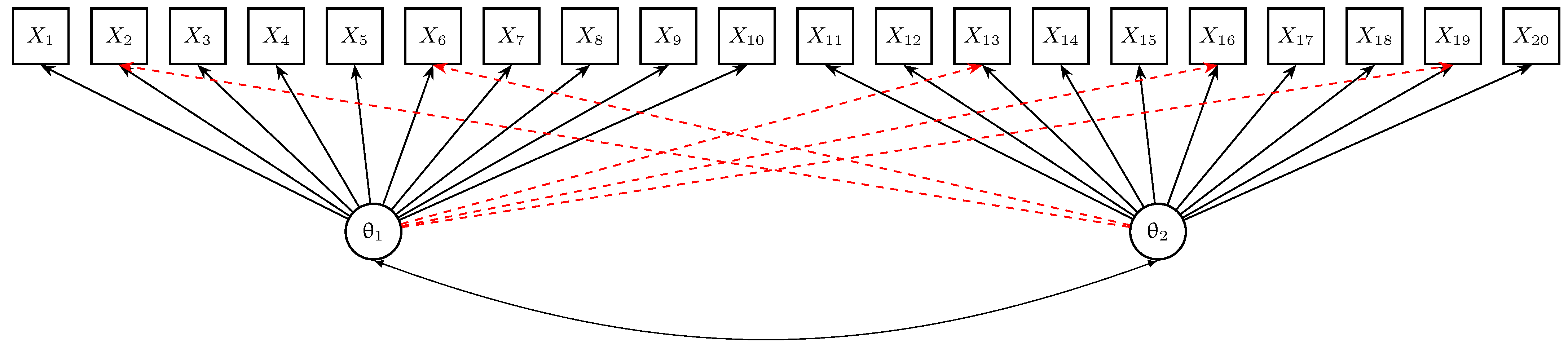
In this simulation study, we used a DGM with $I=20$ items and $D=2$ factor variables ${\mathsf{\theta }}_1$ and ${\mathsf{\theta }}_2$. The first 10 items loaded on the first dimension, while Items 11 to 20 loaded on the second dimension. The factor variable $({\mathsf{\theta }}_1,{\mathsf{\theta }}_2)$ was bivariate normally distributed with standardized normally distributed components and a fixed correlation $\mathsf{\rho }$ of 0.5.

Moreover, we specified five cross-loadings. Items 2 and 6 had a cross-loading of size $\mathsf{\delta }$ on the second dimension, while Items 13, 16, and 19 had a cross-loading of size $\mathsf{\delta }$ on the first dimension. The DGM is visualized in Figure 1. In more detail, the loading matrix $\mathit{A}$ that contains the item discriminations $a_{id}$ (see (18)) is given by

$$\mathbf{A}=\left(\begin{array}{cc}0.6& 0\\ 0.8& \mathsf{\delta }\\ 1.0& 0\\ 1.4& 0\\ 1.2& 0\\ 0.6& \mathsf{\delta }\\ 0.8& 0\\ 1.0& 0\\ 1.4& 0\\ 1.2& 0\\ 0& 0.6\\ 0& 0.8\\ \mathsf{\delta }& 1.0\\ 0& 1.4\\ 0& 1.2\\ \mathsf{\delta }& 0.6\\ 0& 0.8\\ 0& 1.0\\ \mathsf{\delta }& 1.4\\ 0& 1.2\end{array}\right).$$

(19)

The size of the cross-loading $\mathsf{\delta }$ was chosen as 0.3, indicating a small cross-loading), or 0.5, indicating a large cross-loading. The item difficulties $b_i$ (see (18)) of the 20 items were −0.8, 0.4, 1.2, 2.0, −2.0, −0.8, 0.4, 1.2, 2.0, −2.0, −0.8, 0.4, 1.2, 2.0, −2.0, −0.8, 0.4, 1.2, 2.0, and −2.0. The item parameters can also be found at https://osf.io/ykew6 (accessed on 2 April 2024).

We varied the sample size N as 500, 1000, and 2000, which may be interpreted as a small, moderate, and large sample size.

Like in Simulation Study 1, we compared the performance of regularized estimation based on AIC and BIC with the smooth alternatives SAIC and SBIC. A nonequidistant grid of 37 $\mathsf{\lambda }$ values between 0.0001 and 1 was chosen (see the R simulation code at https://osf.io/ykew6; accessed on 2 April 2024). The optimization functions were specified with the same tuning parameters for differentiable approximations as in Simulation Study 1 (see Section 3.1). (Average) absolute bias and (average) RMSE of model parameters, as well as type-I error rates and power rates for cross-loadings, were assessed for the four estimation methods.

In total, $R=750$ replications were conducted in each of the 2 (small vs. large cross-loadings) × 3 (sample size) $=6$ cells of the simulation study. The whole simulation study was conducted using the statistical software R [44]. The estimation of the regularized multidimensional logistic IRT model was carried out using the sirt::xxirt() function in the R package sirt [45]. Replication material for this simulation study can also be found at https://osf.io/ykew6 (accessed on 2 April 2024).

4.2. Results

Table 3. Simulation Study 2: (Average) absolute bias and average root mean square error (RMSE) of model parameters as a function of the size of cross-loadings and sample size N.

			Absolute Bias				RMSE
Par	CL	$\mathit{N}$	AIC	SAIC	BIC	SBIC	AIC	SAIC	BIC	SBIC
$\mathsf{\rho }$		500	0.064	0.054	0.104	0.070	0.151	0.102	0.134	0.110
	small	1000	0.040	0.070	0.088	0.085	0.157	0.096	0.124	0.104
		2000	0.015	0.018	0.059	0.065	0.077	0.052	0.082	0.081
		500	0.055	0.062	0.136	0.073	0.167	0.109	0.179	0.117
	large	1000	0.029	0.054	0.074	0.057	0.144	0.100	0.124	0.099
		2000	0.010	0.014	0.016	0.014	0.062	0.047	0.058	0.051
$CL=0$		500	0.041	0.016	0.015	0.008	0.243	0.113	0.130	0.095
	small	1000	0.025	0.028	0.008	0.014	0.188	0.119	0.092	0.088
		2000	0.011	0.006	0.006	0.003	0.102	0.062	0.049	0.034
		500	0.044	0.016	0.024	0.011	0.282	0.119	0.181	0.109
	large	1000	0.027	0.028	0.013	0.015	0.183	0.127	0.096	0.095
		2000	0.009	0.009	0.005	0.002	0.094	0.067	0.049	0.030
$CL\ne 0$		500	0.102	0.141	0.238	0.177	0.287	0.287	0.306	0.296
	small	1000	0.075	0.118	0.211	0.192	0.237	0.235	0.288	0.273
		2000	0.021	0.033	0.132	0.154	0.140	0.146	0.231	0.243
		500	0.078	0.130	0.295	0.166	0.341	0.353	0.452	0.379
	large	1000	0.036	0.066	0.151	0.107	0.228	0.245	0.336	0.291
		2000	0.011	0.009	0.025	0.028	0.123	0.116	0.161	0.161

Note. Par = parameter; $\mathsf{\rho }$ = correlation between factors ${\mathsf{\theta }}_1$ and ${\mathsf{\theta }}_2$; $CL=0$ = cross-loading with zero population value; $CL\ne 0$ = cross-loading with non-zero population value; Absolute bias values larger than 0.03 are printed in bold font.

reports the (average) absolute bias and (average) RMSE of estimated model parameters. It turned out that the factor correlation $\mathsf{\rho }$ was biased for small and moderate sample sizes of $N=500$ and $N=1000$. The bias was reduced with larger cross-loadings in large sample sizes. However, a notable bias was even present for a large sample size $N=2000$ if the BIC or SBIC was used. However, AIC and SAIC outperformed the other criteria for estimates of $\mathsf{\rho }$ with respect to bias and RMSE. Interestingly, the RMSE of SAIC was substantially smaller compared to AIC for the factor correlation $\mathsf{\rho }$, as well as for true zero cross-loadings (i.e., rows “$CL=0$” in Table 3) and non-zero cross-loadings (i.e., rows “$CL\ne 0$” in Table 3).

Table 4. Simulation Study 2: Type-I error rate and power rate for cross-loadings as a function of the size of cross-loadings and sample size N.

		Type-I Error Rate				Power Rate
CL	$\mathit{N}$	AIC	SAIC	BIC	SBIC	AIC	SAIC	BIC	SBIC
	500	16.7	5.1	2.1	2.5	41.2	30.6	9.4	22.4
small	1000	18.7	8.8	2.0	3.2	58.0	46.5	17.9	24.3
	2000	15.1	6.2	1.7	0.7	86.5	82.4	44.0	38.3
	500	18.5	4.8	3.1	2.8	68.5	59.5	27.3	52.0
large	1000	17.0	10.0	2.5	3.2	87.4	81.0	59.2	70.6
	2000	13.3	7.8	1.3	0.7	98.6	98.7	92.3	92.6

Note. CL = size of cross-loadings; Type-I error rates larger than 10.0 and power rates smaller than 80.0 are printed in bold font.

shows type-I error rates and power rates of estimated cross-loadings. It is evident that AIC had inflated type-I error rates, while type-I error rates of SAIC, BIC, and SBIC were acceptable. Importantly, there were low power rates for BIC and SBIC, in particular for small cross-loadings. The SAIC estimation method may be preferred if the goal is detecting non-zero cross-loadings.

5. Simulation Study 3: Mixed Rasch/2PL Model

Recently, a mixed Rasch/2PL model [52] (see also [53]) received some attention. The idea of this unidimensional IRT model is to find items that conform to the Rasch model [54], while there can be a subset of items that follow the more complex 2PL model [9]. The IRF of this model is given by

$$\mathsf{P}(X_i=1|\mathsf{\theta })=\mathsf{\Psi }\left(exp\left({\mathsf{\alpha }}_i\right)\mathsf{\theta }-b_i\right).$$

(20)

Note that the IRF in (20) is just a reparametrized 2PL model with item discriminations $a_i=exp\left({\mathsf{\alpha }}_i\right)$. Hence, ${\mathsf{\alpha }}_i=log\left(a_i\right)$ are the logarithms of item discriminations $a_i$. The case ${\mathsf{\alpha }}_i=0$ corresponds to the Rasch model because $a_i=exp\left({\mathsf{\alpha }}_i\right)=1$, while ${\mathsf{\alpha }}_i\ne 0$ results in item discriminations $a_i$ different from 1. The mean of the factor variable $\mathsf{\theta }$ is fixed to 0, while the standard deviation $\mathsf{\sigma }$ should be estimated.

In order to achieve identifiability of the model parameters, a sparsity structure of the logarithms of item discriminations ${\mathsf{\alpha }}_i$ is imposed. Hence, the majority of items is assumed to follow the Rasch model. Again, the sparsity structure is directly implemented in a regularized estimation of the mixed Rasch/2PL model.

5.1. Method

In this simulation study, we used $I=20$ items for the DGM of the mixed Rasch/2PL model. The factor variable $\mathsf{\theta }$ was assumed to be normally distributed with a zero mean and a standard deviation $\mathsf{\sigma }=1.2$. The item difficulties $b_i$ (see the IRF in (20)) of the 20 items were chosen as −0.8, 0.4, 1.2, 2.0, −2.0, −0.8, 0.4, 1.2, 2.0, −2.0, −0.8, 0.4, 1.2, 2.0, −2.0, −0.8, 0.4, 1.2, 2.0, and −2.0. The first 14 items followed the Rasch model (i.e., ${\mathsf{\alpha }}_i=0$ for $i=1,\dots ,15$). Items 15 to 20 followed the 2PL model and had ${\mathsf{\alpha }}_i$ values that equaled $-\mathsf{\delta }$, $\mathsf{\delta }$, $-\mathsf{\delta }$, $\mathsf{\delta }$, $\mathsf{\delta }$, and $-\mathsf{\delta }$. The size of $\mathsf{\delta }$ controlled the deviation from the Rasch model. We either chose $\mathsf{\delta }$ as $log\left(1.4\right)=0.336$ and $log\left(2\right)=0.693$, indicating small and large deviations from the Rasch model. Moreover, we manipulated the direction of the deviation from the Rasch model. While the previously described conditions had ${\mathsf{\alpha }}_i$ that canceled out on average and resulted in a balanced deviation from the Rasch model (i.e., there was an equal number of items that are smaller and larger than 1, respectively), we also specified an unbalanced deviation from the Rasch model in which Items 15 to 20 all had the value $\mathsf{\delta }$. In this condition, we also studied small (i.e., $\mathsf{\delta }=0.336$) and large (i.e., $\mathsf{\delta }=0.693$) deviations from the Rasch model. Hence, in the case of unbalanced deviations from the Rasch model, items had either discriminations of 1 or larger than 1. The item parameters can also be found at https://osf.io/ykew6 (accessed on 2 April 2024).

Like in the other two simulation studies, we varied the sample size N as 500, 1000, and 2000.

Again, like in Simulation Study 1 and Simulation Study 2, we compared the performance of regularized estimation based on AIC and BIC with the smooth alternatives SAIC and SBIC. A nonequidistant grid of 33 $\mathsf{\lambda }$ values between 0.001 and 1 was chosen (see the R simulation code at https://osf.io/ykew6; accessed on 2 April 2024). The optimization functions were specified with the same tuning parameters for differentiable approximations as in Simulation Study 1 (see Section 3.1). (Average) absolute bias and (average) RMSE of model parameters $\mathsf{\sigma }$ and ${\mathsf{\alpha }}_i$ ($i=1,\dots ,I$), as well as type-I error rates and power rates for logarithms of item discriminations, were assessed.

Overall, $R=750$ replications were conducted in each of the 2 (small vs. large deviations) × 2 (balanced vs. unbalanced deviations) × 3 (sample size) $=12$ cells of the simulation study. This simulation study was also executed using the statistical software R [44]. Like in the other two simulation studies, the regularized multidimensional logistic IRT model was estimated using the sirt::xxirt() function in the R package sirt [45]. Replication material for this simulation study can also be found at https://osf.io/ykew6 (accessed on 2 April 2024).

5.2. Results

Table 5. Simulation Study 3: (Average) absolute bias and average root mean square error (RMSE) of model parameters as a function of the sample size N and the size and the extent and direction of deviations from the Rasch model.

			(Average) Absolute Bias				(Average) RMSE
Par	Dev	$\mathit{N}$	AIC	SAIC	BIC	SBIC	AIC	SAIC	BIC	SBIC
			Balanced deviations from the Rasch model
$\mathsf{\sigma }$		500	0.053	0.038	0.004	0.010	0.099	0.082	0.070	0.072
	small	1000	0.062	0.005	0.012	0.004	0.107	0.054	0.051	0.056
		2000	0.109	0.001	0.025	0.009	0.167	0.032	0.044	0.037
		500	0.018	0.014	0.004	0.006	0.069	0.065	0.064	0.064
	large	1000	0.016	0.002	0.002	0.002	0.050	0.044	0.041	0.041
		2000	0.007	0.000	0.000	0.000	0.035	0.033	0.030	0.030
${\mathsf{\alpha }}_i=0$		500	0.035	0.017	0.001	0.002	0.124	0.091	0.048	0.047
	small	1000	0.048	0.003	0.002	0.001	0.119	0.060	0.027	0.020
		2000	0.096	0.001	0.003	0.000	0.166	0.042	0.023	0.003
		500	0.018	0.012	0.002	0.002	0.101	0.082	0.046	0.044
	large	1000	0.017	0.003	0.001	0.000	0.066	0.058	0.023	0.014
		2000	0.007	0.001	0.000	0.000	0.033	0.040	0.010	0.003
${\mathsf{\alpha }}_i\ne 0$		500	0.071	0.070	0.127	0.137	0.224	0.239	0.283	0.289
	small	1000	0.081	0.024	0.075	0.101	0.184	0.154	0.212	0.237
		2000	0.120	0.003	0.072	0.045	0.199	0.085	0.159	0.156
		500	0.014	0.017	0.015	0.018	0.207	0.215	0.230	0.231
	large	1000	0.019	0.006	0.006	0.008	0.139	0.136	0.138	0.143
		2000	0.004	0.004	0.003	0.004	0.095	0.095	0.093	0.094
			Unbalanced deviations from the Rasch model
$\mathsf{\sigma }$		500	0.008	0.032	0.084	0.083	0.076	0.081	0.110	0.109
	small	1000	0.015	0.008	0.028	0.055	0.051	0.050	0.061	0.078
		2000	0.011	0.003	0.002	0.015	0.036	0.032	0.031	0.040
		500	0.001	0.001	0.001	0.001	0.069	0.062	0.061	0.060
	large	1000	0.005	0.001	0.000	0.001	0.046	0.043	0.040	0.040
		2000	0.002	0.003	0.002	0.002	0.034	0.032	0.030	0.029
${\mathsf{\alpha }}_i=0$		500	0.009	0.005	0.008	0.004	0.099	0.078	0.057	0.047
	small	1000	0.014	0.003	0.002	0.001	0.068	0.056	0.027	0.019
		2000	0.010	0.002	0.001	0.000	0.044	0.042	0.015	0.005
		500	0.003	0.003	0.001	0.001	0.105	0.079	0.046	0.041
	large	1000	0.004	0.001	0.001	0.000	0.069	0.053	0.025	0.013
		2000	0.003	0.001	0.001	0.000	0.047	0.039	0.014	0.002
${\mathsf{\alpha }}_i\ne 0$		500	0.029	0.069	0.194	0.205	0.180	0.207	0.281	0.289
	small	1000	0.012	0.014	0.069	0.145	0.103	0.116	0.182	0.240
		2000	0.012	0.001	0.002	0.037	0.068	0.067	0.075	0.129
		500	0.008	0.006	0.007	0.005	0.129	0.126	0.127	0.127
	large	1000	0.011	0.007	0.006	0.006	0.091	0.089	0.089	0.089
		2000	0.003	0.003	0.003	0.003	0.062	0.061	0.061	0.061

Note. Par = parameter; Dev = size of deviation from the Rasch model; σ = standard deviation of factor variable θ; α_i = 0 = logarithm of item discriminations with zero population value; α_i ≠0 = logarithm of item discriminations with non-zero population value; Absolute bias values larger than 0.03 are printed in bold font.

contains the (average) absolute bias and (average) RMSE for the estimated model parameters. Notably, there was a different pattern of findings in the conditions of balanced and unbalanced deviations from the Rasch model. In general, SAIC performed well for the estimation of $\mathsf{\sigma }$, except for small balanced deviations from the Rasch model with a sample size of $N=500$. In most of the conditions, estimation based on SBIC performed similarly, if not better, than BIC for the estimation of $\mathsf{\sigma }$ in terms of RMSE.

Table 6. Simulation Study 3: Type-I error rate and power rate for logarithm of item discriminations as a function of the sample size N and the size and the extent and direction of deviations from the Rasch model.

		Type-I Error Rate				Power Rate
Dev	$\mathit{N}$	AIC	SAIC	BIC	SBIC	AIC	SAIC	BIC	SBIC
		Balanced deviations from the Rasch model
	500	14.6	7.7	1.3	1.2	68.8	61.6	40.6	39.6
small	1000	18.5	6.5	0.7	0.3	77.6	85.5	63.6	55.9
	2000	36.4	7.7	0.6	0.0	78.8	98.7	75.5	79.8
	500	11.4	6.6	1.3	1.2	97.9	95.8	93.8	93.6
large	1000	9.3	6.6	0.6	0.2	99.7	99.8	99.4	98.9
	2000	4.4	7.4	0.1	0.0	100	100	100	100
		Unbalanced deviations from the Rasch model
	500	11.4	5.7	1.8	1.1	80.4	69.5	30.9	29.9
small	1000	10.8	5.9	0.8	0.3	97.9	94.0	72.5	50.9
	2000	8.3	7.7	0.4	0.1	99.9	99.9	98.2	87.3
	500	13.7	5.9	1.2	1.0	100	100	99.9	99.9
large	1000	12.1	5.8	0.7	0.2	100	100	100	100
	2000	10.9	7.3	0.4	0.0	100	100	100	100

Note. Dev = size of deviation from the Rasch model; Type-I error rates larger than 10.0 and power rates smaller than 80.0 are printed in bold font.

displays type-I error rates and power rates for estimated logarithms of item discriminations. In contrast to the estimation based on the AIC, SAIC had acceptable type-I error rates. Moreover, power rates for detecting deviations from the Rasch model were much higher for SAIC then BIC or SBIC.

6. Discussion

In this article, we compared the ordinarily employed indirect regularized estimation based on a grid of regularization parameters $\mathsf{\lambda }$ with a subsequent discrete minimization of AIC and BIC with a direct minimization of smooth information criteria SAIC and SBIC [26] for the estimation of regularized item response models. It turned out that the direct SIC-based estimation methods resulted in comparable, in many cases, or better performance than the indirect regularization estimation methods based on AIC and BIC. This is remarkable because SIC-based minimization is computationally much simpler, and ordinary gradient-based optimization routines can be utilized.

We studied the performance of SAIC and SBIC in three simulation studies that focus on differential item functioning, (semi-)exploratory multidimensional IRT models, and model choice between the Rasch model and the 2PL model. These three cases frequently appear in applications of regularized IRT models, which is why we chose these settings for our work.

In this article, we confined ourselves to analyzing dichotomous item responses and continuous factor variables. Future research could investigate the application of these techniques to polytomous item response, count item response data [55], or cognitive diagnostic models that involve multivariate binary factor variables [56]. More generally, smooth information criteria can be used in all modeling approaches that involve regularized estimation. In the field of econometrics or social science, possible applications could be (generalized) linear regression models [57], regularized panel models [58], or regularized estimation for analyzing heterogeneous treatment effects [59].

Notably, we did not investigate the estimation of standard errors in this article. Future research may investigate this with an application of the Huber–White variance estimation formula [60,61] applied to the subset of parameters that resulted in non-zero values [62].

Finally, two different targets in the analysis of item response models should be distinguished in regularized estimation. First, the selection or detection of non-zero effects like cross-loadings or DIF effects may be the focus. For this goal, model selection based on information criteria can prove helpful in order to control type-I error rates. Second, if the focus lies on structural parameters (such as group means or factor correlations), choosing a parsimonious model that tries to penalize the number of estimated parameters, like in information criteria, may not be beneficial in terms of bias and variability of structural parameters [21]. It can be advantageous to use a sufficiently small regularization parameter $\mathsf{\lambda }$ to ensure the empirical identifiability of the model but not to focus on effect selection if structural parameters are of interest [63]. In this sense, sparsity in effects is imposed in a defensive way.

References

- Baker, F.B.; Kim, S.H. Item Response Theory: Parameter Estimation Techniques; CRC Press: Boca Raton, FL, USA, 2004. [Google Scholar] [CrossRef]
- Bock, R.D.; Gibbons, R.D. Item Response Theory; Wiley: Hoboken, NJ, USA, 2021. [Google Scholar] [CrossRef]
- Chen, Y.; Li, X.; Liu, J.; Ying, Z. Item response theory—A statistical framework for educational and psychological measurement. arXiv 2021, arXiv:2108.08604. [Google Scholar]
- van der Linden, W.J.; Hambleton, R.K. (Eds.) Handbook of Modern Item Response Theory; Springer: New York, NY, USA, 1997. [Google Scholar] [CrossRef]
- Yen, W.M.; Fitzpatrick, A.R. Item response theory. In Educational Measurement; Brennan, R.L., Ed.; Praeger Publishers: Westport, CT, USA, 2006; pp. 111–154. [Google Scholar]
- van der Linden, W.J. Unidimensional logistic response models. In Handbook of Item Response Theory, Volume 1: Models; van der Linden, W.J., Ed.; CRC Press: Boca Raton, FL, USA, 2016; pp. 11–30. [Google Scholar]
- Reckase, M.D. Logistic multidimensional models. In Handbook of Item Response Theory, Volume 1: Models; van der Linden, W.J., Ed.; CRC Press: Boca Raton, FL, USA, 2016; pp. 189–210. [Google Scholar]
- Swaminathan, H.; Rogers, H.J. Normal-ogive multidimensional models. In Handbook of Item Response Theory, Volume 1: Models; van der Linden, W.J., Ed.; CRC Press: Boca Raton, FL, USA, 2016; pp. 167–187. [Google Scholar]
- Birnbaum, A. Some latent trait models and their use in inferring an examinee’s ability. In Statistical Theories of Mental Test Scores; Lord, F.M., Novick, M.R., Eds.; MIT Press: Reading, MA, USA, 1968; pp. 397–479. [Google Scholar]
- Fan, J.; Li, R.; Zhang, C.H.; Zou, H. Statistical Foundations of Data Science; Chapman and Hall/CRC: Boca Raton, FL, USA, 2020. [Google Scholar] [CrossRef]
- Goretzko, D.; Bühner, M. Note: Machine learning modeling and optimization techniques in psychological assessment. Psychol. Test Assess. Model. 2022, 64, 3–21. Available online: https://tinyurl.com/bdehjkzz (accessed on 2 April 2024).
- Finch, H. Applied Regularization Methods for the Social Sciences; Chapman and Hall/CRC: Boca Raton, FL, USA, 2022. [Google Scholar] [CrossRef]
- Jacobucci, R.; Grimm, K.J.; Zhang, Z. Machine Learning for Social and Behavioral Research; Guilford Publications: New York, NY, USA, 2023. [Google Scholar]
- Hastie, T.; Tibshirani, R.; Wainwright, M. Statistical Learning with Sparsity: The Lasso and Generalizations; CRC Press: Boca Raton, FL, USA, 2015. [Google Scholar] [CrossRef]
- Fan, J.; Li, R. Variable selection via nonconcave penalized likelihood and its oracle properties. J. Am. Stat. Assoc. 2001, 96, 1348–1360. [Google Scholar] [CrossRef]
- Zhang, H.; Li, S.J.; Zhang, H.; Yang, Z.Y.; Ren, Y.Q.; Xia, L.Y.; Liang, Y. Meta-analysis based on nonconvex regularization. Sci. Rep. 2020, 10, 5755. [Google Scholar] [CrossRef] [PubMed]
- Orzek, J.H.; Arnold, M.; Voelkle, M.C. Striving for sparsity: On exact and approximate solutions in regularized structural equation models. Struct. Equ. Model. 2023, 30, 956–973. [Google Scholar] [CrossRef]
- Zhang, S.; Chen, Y. Computation for latent variable model estimation: A unified stochastic proximal framework. Psychometrika 2022, 87, 1473–1502. [Google Scholar] [CrossRef] [PubMed]
- Battauz, M. Regularized estimation of the nominal response model. Multivar. Behav. Res. 2020, 55, 811–824. [Google Scholar] [CrossRef] [PubMed]
- Oelker, M.R.; Tutz, G. A uniform framework for the combination of penalties in generalized structured models. Adv. Data Anal. Classif. 2017, 11, 97–120. [Google Scholar] [CrossRef]
- Robitzsch, A. Implementation aspects in regularized structural equation models. Algorithms 2023, 16, 446. [Google Scholar] [CrossRef]
- Robitzsch, A. Model-robust estimation of multiple-group structural equation models. Algorithms 2023, 16, 210. [Google Scholar] [CrossRef]
- Cavanaugh, J.E.; Neath, A.A. The Akaike information criterion: Background, derivation, properties, application, interpretation, and refinements. WIREs Comput. Stat. 2019, 11, e1460. [Google Scholar] [CrossRef]
- Neath, A.A.; Cavanaugh, J.E. The Bayesian information criterion: Background, derivation, and applications. WIREs Comput. Stat. 2012, 4, 199–203. [Google Scholar] [CrossRef]
- Burnham, K.P.; Anderson, D.R. Model Selection and Multimodel Inference: A Practical Information-Theoretic Approach; Springer: New York, NY, USA, 2002. [Google Scholar] [CrossRef]
- O’Neill, M.; Burke, K. Variable selection using a smooth information criterion for distributional regression models. Stat. Comput. 2023, 33, 71. [Google Scholar] [CrossRef] [PubMed]
- Bollen, K.A.; Noble, M.D. Structural equation models and the quantification of behavior. Proc. Natl. Acad. Sci. USA 2011, 108, 15639–15646. [Google Scholar] [CrossRef] [PubMed]
- Oelker, M.R.; Pößnecker, W.; Tutz, G. Selection and fusion of categorical predictors with L0-type penalties. Stat. Model. 2015, 15, 389–410. [Google Scholar] [CrossRef]
- Shen, X.; Pan, W.; Zhu, Y. Likelihood-based selection and sharp parameter estimation. J. Am. Stat. Assoc. 2012, 107, 223–232. [Google Scholar] [CrossRef] [PubMed]
- Holland, P.W.; Wainer, H. (Eds.) Differential Item Functioning: Theory and Practice; Lawrence Erlbaum: Hillsdale, NJ, USA, 1993. [Google Scholar] [CrossRef]
- Mellenbergh, G.J. Item bias and item response theory. Int. J. Educ. Res. 1989, 13, 127–143. [Google Scholar] [CrossRef]
- Millsap, R.E. Statistical Approaches to Measurement Invariance; Routledge: New York, NY, USA, 2011. [Google Scholar] [CrossRef]
- Bechger, T.M.; Maris, G. A statistical test for differential item pair functioning. Psychometrika 2015, 80, 317–340. [Google Scholar] [CrossRef] [PubMed]
- Doebler, A. Looking at DIF from a new perspective: A structure-based approach acknowledging inherent indefinability. Appl. Psychol. Meas. 2019, 43, 303–321. [Google Scholar] [CrossRef] [PubMed]
- San Martin, E. Identification of item response theory models. In Handbook of Item Response Theory, Volume 2: Statistical Tools; van der Linden, W.J., Ed.; CRC Press: Boca Raton, FL, USA, 2016; pp. 127–150. [Google Scholar] [CrossRef]
- Belzak, W.; Bauer, D.J. Improving the assessment of measurement invariance: Using regularization to select anchor items and identify differential item functioning. Psychol. Methods 2020, 25, 673–690. [Google Scholar] [CrossRef] [PubMed]
- Belzak, W.C.M.; Bauer, D.J. Using regularization to identify measurement bias across multiple background characteristics: A penalized expectation-maximization algorithm. J. Educ. Behav. Stat. 2024. Epub ahead of print. [Google Scholar] [CrossRef]
- Chen, Y.; Li, C.; Ouyang, J.; Xu, G. DIF statistical inference without knowing anchoring items. Psychometrika 2023, 88, 1097–1122. [Google Scholar] [CrossRef] [PubMed]
- Robitzsch, A. Comparing robust linking and regularized estimation for linking two groups in the 1PL and 2PL models in the presence of sparse uniform differential item functioning. Stats 2023, 6, 192–208. [Google Scholar] [CrossRef]
- Schauberger, G.; Mair, P. A regularization approach for the detection of differential item functioning in generalized partial credit models. Behav. Res. Methods 2020, 52, 279–294. [Google Scholar] [CrossRef] [PubMed]
- Tutz, G.; Schauberger, G. A penalty approach to differential item functioning in Rasch models. Psychometrika 2015, 80, 21–43. [Google Scholar] [CrossRef]
- Wang, C.; Zhu, R.; Xu, G. Using lasso and adaptive lasso to identify DIF in multidimensional 2PL models. Multivar. Behav. Res. 2023, 58, 387–407. [Google Scholar] [CrossRef] [PubMed]
- Pohl, S.; Schulze, D.; Stets, E. Partial measurement invariance: Extending and evaluating the cluster approach for identifying anchor items. Appl. Psychol. Meas. 2021, 45, 477–493. [Google Scholar] [CrossRef] [PubMed]
- R Core Team. R: A Language and Environment for Statistical Computing; R Foundation: Vienna, Austria, 2023; Available online: https://www.R-project.org/ (accessed on 15 March 2023).
- Robitzsch, A. sirt: Supplementary Item Response Theory Models. 2024. R Package Version 4.1-15. Available online: https://CRAN.R-project.org/package=sirt (accessed on 6 February 2024.).
- Reckase, M.D. Multidimensional Item Response Theory Models; Springer: New York, NY, USA, 2009. [Google Scholar] [CrossRef]
- Chen, J. A partially confirmatory approach to the multidimensional item response theory with the Bayesian lasso. Psychometrika 2020, 85, 738–774. [Google Scholar] [CrossRef] [PubMed]
- Chen, Y.; Li, X.; Liu, J.; Ying, Z. Robust measurement via a fused latent and graphical item response theory model. Psychometrika 2018, 83, 538–562. [Google Scholar] [CrossRef] [PubMed]
- Sun, J.; Chen, Y.; Liu, J.; Ying, Z.; Xin, T. Latent variable selection for multidimensional item response theory models via L1 regularization. Psychometrika 2016, 81, 921–939. [Google Scholar] [CrossRef]
- Goretzko, D. Regularized exploratory factor analysis as an alternative to factor rotation. Eur. J. Psychol. Assess. 2023. Epub ahead of print. [Google Scholar] [CrossRef]
- Scharf, F.; Nestler, S. Should regularization replace simple structure rotation in exploratory factor analysis? Struct. Equ. Modeling 2019, 26, 576–590. [Google Scholar] [CrossRef]
- OECD. PISA 2015. Technical Report; OECD: Paris, France, 2017; Available online: https://bit.ly/32buWnZ (accessed on 2 April 2024).
- Wijayanto, F.; Mul, K.; Groot, P.; van Engelen, B.G.M.; Heskes, T. Semi-automated Rasch analysis using in-plus-out-of-questionnaire log likelihood. Brit. J. Math. Stat. Psychol. 2021, 74, 313–339. [Google Scholar] [CrossRef] [PubMed]
- Rasch, G. Probabilistic Models for Some Intelligence and Attainment Tests; Danish Institute for Educational Research: Copenhagen, Denmark, 1960. [Google Scholar]
- Beisemann, M.; Holling, H.; Doebler, P. Every trait counts: Marginal maximum likelihood estimation for novel multidimensional count data item response models with rotation or L1-regularization for simple structure. PsyArXiv 2024. [Google Scholar] [CrossRef]
- Chen, Y.; Liu, J.; Xu, G.; Ying, Z. Statistical analysis of Q-matrix based diagnostic classification models. J. Am. Stat. Assoc. 2015, 110, 850–866. [Google Scholar] [CrossRef] [PubMed]
- McNeish, D.M. Using lasso for predictor selection and to assuage overfitting: A method long overlooked in behavioral sciences. Multivar. Behav. Res. 2015, 50, 471–484. [Google Scholar] [CrossRef] [PubMed]
- Bai, J. Panel data models with interactive fixed effects. Econometrica 2009, 77, 1229–1279. [Google Scholar] [CrossRef]
- Imai, K.; Ratkovic, M. Estimating treatment effect heterogeneity in randomized program evaluation. Ann. Appl. Stat. 2013, 7, 443–470. [Google Scholar] [CrossRef]
- White, H. Maximum likelihood estimation of misspecified models. Econometrica 1982, 50, 1–25. [Google Scholar] [CrossRef]
- Boos, D.D.; Stefanski, L.A. Essential Statistical Inference; Springer: New York, NY, USA, 2013. [Google Scholar] [CrossRef]
- Huang, P.H. Penalized least squares for structural equation modeling with ordinal responses. Multivar. Behav. Res. 2022, 57, 279–297. [Google Scholar] [CrossRef] [PubMed]
- Asparouhov, T.; Muthén, B. Penalized structural equation models. Struct. Equ. Modeling 2023. Epub ahead of print. [Google Scholar] [CrossRef]
Figure 1.
Simulation Study 2: Data-generating model with items () and two factor variables and . Cross-loadings are depicted by red dashed lines.