Spike-Weighted Spiking Neural Network with Spiking Long Short-Term Memory: A Biomimetic Approach to Decoding Brain Signals

Abstract

Background. Brain–machine interfaces (BMIs) offer users the ability to directly communicate with digital devices through neural signals decoded with machine learning (ML)-based algorithms. Spiking Neural Networks (SNNs) are a type of Artificial Neural Network (ANN) that operate on neural spikes instead of continuous scalar outputs. Compared to traditional ANNs, SNNs perform fewer computations, use less memory, and mimic biological neurons better. However, SNNs only retain information for short durations, limiting their ability to capture long-term dependencies in time-variant data. Here, we propose a novel spike-weighted SNN with spiking long short-term memory (swSNN-SLSTM) for a regression problem. Spike-weighting captures neuronal firing rate instead of membrane potential, and the SLSTM layer captures long-term dependencies. Methods. We compared the performance of various ML algorithms during decoding directional movements, using a dataset of microelectrode recordings from a macaque during a directional joystick task, and also an open-source dataset. We thus quantified how swSNN-SLSTM performed compared to existing ML models: an unscented Kalman filter, LSTM-based ANN, and membrane-based SNN techniques. Result. The proposed swSNN-SLSTM outperforms both the unscented Kalman filter, the LSTM-based ANN, and the membrane based SNN technique. This shows that incorporating SLSTM can better capture long-term dependencies within neural data. Also, our proposed swSNN-SLSTM algorithm shows promise in reducing power consumption and lowering heat dissipation in implanted BMIs.

1. Introduction

Brain–machine interfaces (BMIs) are devices that acquire brain signals and convert them into computer outputs, for example by using algorithms to map them to computer commands [1,2,3]. A subset of BMIs can map neural activity to movements or movement intentions in humans and non-human primate (NHP) models. These have the potential to improve communication and movement capabilities in humans suffering from paralysis [4,5,6]. BMIs can be classified as invasive or non-invasive. While non-invasive methods are generally less complicated, easier to implement, and have lower risks of serious side-effects, they lack the spatial and temporal resolution of invasive multi-electrode arrays (MEAs), which can be implanted directly into the primary motor cortex and are able to resolve the spikes in individual neurons. Combined with the use of machine learning algorithms to decode the neural activity, these have the potential to create very accurate brain–machine interfaces (BMIs).

Kalman filters (KF) [7] and variants are commonly used as neural decoders, and have successfully been used in many experiments with NHPs [8,9,10], as well as in human clinical trials [11]. However, KFs and its variants suffer from several limitations. KFs are linear by default, while the neuronal activity that they are meant to be decoding has been shown to be non-linear [12]. While extensions like the unscented Kalman filter (UKF) and using a number of ‘taps’ (time bins of spike counts) can reduce these issues, the KF still cannot retain temporal information over a sufficiently long period of time, as too many taps can lead to overfitting [13].

To overcome these issues, recurrent artificial neural networks (RNNs) such as the long short-term memory (LSTM) layer have been used to decode neural information in BMIs [14,15,16]. Artificial neural networks (ANNs) with nonlinear activations are able to model nonlinear functions more closely, and those designed using LSTM layers are able to retain temporal information over an arbitrary number of time steps, leading to a better performance than KFs and modified KFs [14]. However, ANNs greatly increase the computational complexity [17,18], requiring more computational power and electricity, taking more time to train and execute, and generating more heat. High levels of power consumption and heat waste are especially serious problems in the context of implanted BMIs, as even small changes in temperature can cause damage to the sensitive neural tissue [19].

Spiking neural networks (SNNs) [20] are a type of neural network that more accurately mimic actual biological neurons, which communicate through discrete signals (known as action potentials or neural spikes) instead of continuous scalar outputs. In SNNs, the virtual spikes are controlled by membrane potentials using differential equations modelled on biological action potentials [21]. This makes them well-suited to BMI tasks, as the input to the algorithm is already encoded in the form of the recorded neuronal spikes. SNNs have also been shown to require less computational power than traditional ANNs [22,23,24].

However, traditional SNNs, like traditional RNNs, have problems capturing long-term information within data. We have extended the SNN by adding a spiking long short-term memory layer (SLSTM), which can help capture temporal dynamics in the neural data. We hypothesized that it would perform better than current SNN techniques. We also used SNN models with trainable membrane potential thresholds to increase activation sparsity.

Traditionally, when SNNs are used in classification problems [25,26] the spikes are used as the output. However, for regression-based problems, the membrane potential is used as the output [27].

Instead of taking this approach, to further augment the SNN, we introduced a unique output scheme using a linear weighting of output spikes to mimic the biology of the motor cortex more closely. Since the brain communicates using spikes, we hypothesized that this method could perform better than a membrane-based SNN. A spike-weighted SNN would also be less dependent on the starting conditions compared to the membrane potential, which must always start at 0.

In this study we tested two different methods of regression in SNNs (spike-weighted and membrane potential) against two alternative decoders (LSTM [16] and Unscented Kalman filter) [13]. We used each decoder to reconstruct positional data from the input spike data in a regression problem and evaluated their performance by seeing how closely they matched the ground truth, which is the actual joystick positions, using the Pearson correlation coefficient (r) and the coefficient of determination ($R^2$). Kalman filters and LSTMs have previously been used for regression problems in brain–machine interfaces [16].

2. Methods

In this section, we will describe the datasets we analyzed, as well as the ML models we used for decoding.

2.1. Datasets

We tested the models on two datasets. Dataset 1 was collected by us [16]. For Dataset 1, all experimental procedures described in this paper involving animal experimentation were approved by, and conducted in compliance with the standards of, the Agri-Food and Veterinary Authority of Singapore and the Singapore Health Services Institutional Animal Care and Use Committee. Dataset 2 was taken from an open-source dataset, described in [28] and used in [29].

For Dataset 1, an electrode array was implanted in the motor cortex of an adult male macaque (Macaca fascicularis), and recordings were performed as previously described [30,31].

During each recording session, the macaque was positioned in front of a screen while it held a joystick with its left forelimb. For each trial, an audio cue and a cursor appeared in the center of the screen, with a target appearing at 1 of 8 points equidistantly positioned in a ring around the screen center. The macaque was trained to direct the cursor towards the target by moving the joystick. On successful completion of each trial, a reward was delivered in the form of fruit juice. For each recording day, there were 7–8 blocks of recordings, each containing 16–40 trials. Neural activity was recorded in 100 channels at a sampling rate of 30 kHz. Failed trials were excluded from the training and testing datasets, and successful trials were concatenated, then treated as a continuous time series for training and evaluating our models. As the experiment was designed such that each successful trial began and ended at the center, we avoided discontinuities in the joystick position.

All models were coded by authors using Python 3.9.7, Pytorch 2.0.1, and Snntorch 0.6.4.

Signals were first cleaned by having inactive channels (i.e., those with no neural signals) removed from the data set, as these channels introduce more noise and can lead to an inaccurate BMI performance [32]. Common averaging referencing (CAR) was used to reduce cross-channel noise [33] and the signals were filtered between 300 and 3000 Hz. From these signals, action potentials (i.e., neuronal spikes) were detected using a thresholding algorithm, as outlined in [30]. Neuronal activity in each channel was then binned into sliding 500 ms windows, updated every 100 ms. Joystick data were then resampled at 10 Hz to temporally align with the neural spikes. These spike data were then normalized ($\frac{Y-\overline{Y}}{\mathrm{\sigma }}$) so they would fit better into our ANN algorithms.

For joystick position data, all data were normalized, and models were coded by the authors using the modules listed above.

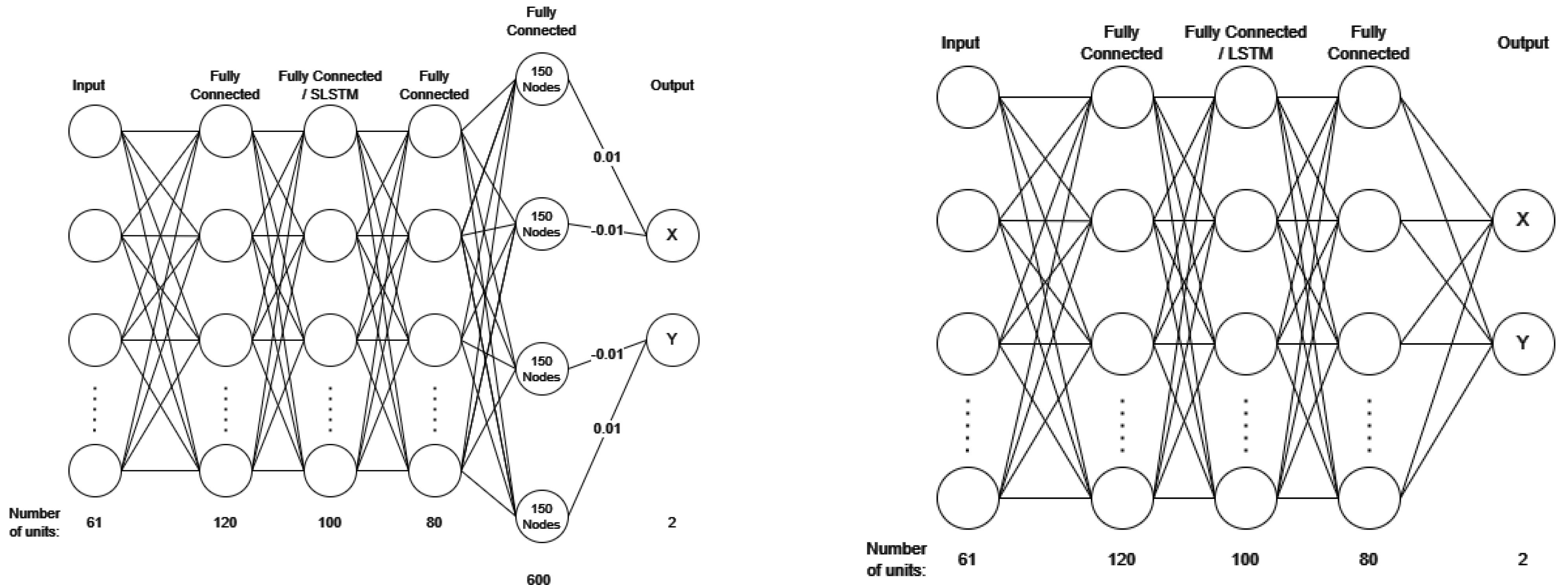
2.2. Decoder Architecture

2.2.1. Spiking Neural Networks

Spiking neural networks [34] are networks that propagate information through discrete spikes, where the spike output is controlled by a membrane potential modelled on differential equations. They can be trained in three distinct ways:

(1)

Conversion from ANNs to SNNs; however, this can cause issues, leading to the need to increase the time period for inference latency [35].

(2)

Using a biologically plausible approach called spike-timing-dependent plasticity (STDP) [36]. This, however, has exhibited problems in terms of performance.

(3)

Backpropagation through time (BPTT), which was the method we used. BPTT uses surrogate gradients in the backwards pass to allow for differentiability [34].

For this method, we used two different models of neurons. The main model used in this study is the leaky integrate and fire (LIF) model:

$$\mathrm{U}\left[T+1\right]=\underset{decay}{\mathrm{\beta }U\left[T\right]}+\underset{input}{WX\left[T+1\right]}-\underset{reset}{S\left[T\right]U_{thr}}$$

(1)

However, we also undertook a brief comparison with the Synaptic current-based LIF model:

$$\begin{array}{c}{I}_{syn}\left[T+1\right]=\underset{decay}{\mathrm{\alpha }{I}_{syn\left[T\right]}}+\underset{input}{WX\left[T+1\right]}\\ U\left[T+1\right]=\underset{decay}{\mathrm{\beta }U\left[T\right]}+\underset{input}{I_{syn}\left[T+1\right]}-\underset{reset}{R\left[T\right]}\end{array}$$

(2)

Spikes are governed by the following equation:

$$S_{out}\left[T\right]=\begin{array}{c}1ifU\left[T\right]>U_{thr}\\ 0\end{array}$$

(3)

where $\mathrm{\alpha }$ = the decay rate of the synaptic current; $\mathrm{\beta }$ = the decay rate of the membrane potential; $U$ = membrane potential; $I_{syn}$ = synaptic current; $W$ = weights; $T$ is a discrete variable representing the current timestep; $X$ represents the data being passed to the neuron.

2.2.2. Spiking Long Short-Term Memory (SLSTM) Architecture

We used the SLSTM architecture, as described in [23]. This is comparable to the general LSTM architecture [37], but only one time step is simulated each time the cell is called. The forward pass is governed by the following equations:

$$\begin{array}{c}\begin{array}{c}{i}_T=\mathrm{\sigma }\left(W_{ii}X\left[T+1\right]+b_{ii}+W_{hi}U\left[T\right]+b_{hi}\right)\\ f_T=\mathrm{\sigma }\left(W_{if}X\left[T+1\right]+b_{if}+W_{hf}U\left[T\right]+b_{hf}\right)\\ g_T=\tanh \left(W_{ig}X\left[T+1\right]+b_{ig}+W_{hg}U\left[T\right]+b_{hg}\right)\\ o_T=\mathrm{\sigma }\left(W_{io}X\left[T+1\right]+b_{io}+W_{ho}U\left[T\right]+b_{ho}\right)\\ I_{syn}\left[T+1\right]=f_T\star I_{syn}\left[T\right]+i_T\star g_T\\ U\left[T+1\right]=o_T\star tanh\left(I_{syn}\left[T+1\right]\right)\end{array}\end{array}$$

(4)

In the original LSTM formulation $h,c$ are the hidden and cell states, which correspond to $U$ and $I_{syn}$ in the SLSTM formulation. In the equation presented above, $\mathrm{\sigma }$ is the sigmoid function and $\star$ is the Hadamard product. The input gate $i_T$ determines the information added to the memory cells, the forget gate $f_T$ determines the information to be forgotten, and $o_T$ determines if the memory cell state $I_{syn}$ should cause an output spike (as long as $U\left[T+1\right]>U_{thr}$). $b$ and $W$ correspond to the learnable biases and weights. In the SLSTM, the reset scheme is set to ‘none’.

2.2.3. Spiking Decoders

We constructed two different output types of spiking neural networks: one spike-weighted decoder and another based on membrane potential:

Each output type had two different model makeups, using either a spiking LSTM model or a fully connected model. This created four different models: spike-weighted SNN (swSNN), spike-weighted SLSTM (swSNN-SLSTM), membrane potential SNN (memSNN), and membrane potential SLSTM (memSNN-SLSTM).

The models were all constructed using the LIF neuron and reset via subtraction scheme instead of resetting to zero for membrane potential, as inspired by [38]. The ‘Arctan’ surrogate gradient ($\overline{S}=\frac{1}{\mathsf{\pi }}\mathrm{a}\mathrm{r}\mathrm{c}\mathrm{t}\mathrm{a}\mathrm{n}\left(\mathsf{\pi }U\right)$) was used, as proposed by [39]. All layers had learnable threshold and beta parameters, as well as a dropout layer after the first three layers to prevent overfitting [40].

An Adam optimizer [41] was used with $\mathrm{\beta }=\left(0.9,0.999\right)$, $\mathsf{ϵ}=$ 10⁻⁸. A Reduce LR On Plateau Scheduler was used with patience = 8, factor = 0.5, and mode = ‘min’, and a mean square error loss function was used. The neuron parameters outlined below were initialized as tensors, where the value was just the initial tensor size.

For all models, the input was the normalized spike data in discrete time steps, and the output represented the decoded joystick position variables in the corresponding time steps.

The spike-weighted model’s architecture is shown on the left of Figure 1, with the last fully connected layer having 600 nodes. This effectively acted as an output layer, as it had fixed weight connections into the joystick output. The output spikes were summed and scaled, either positively or negatively, by 0.01 to give the x and y joystick values. The value of 0.01 was chosen as this was the resolution of the original data, and 600 nodes were used to over-encompass the range of −1–1, as the joystick data varied within this range. The reason we chose 600 is because there was no significant difference in model accuracy between 400 and 800 nodes (see Section 3.2), so we decided to use the value that was in the middle of the feasible region we tested. Note there are only 300 nodes for each variable, as nodes are not shared, and half of these nodes are negative, so the max value is only 1.5. Over-encompassing also means that the model does not need to output a spike at every neuron if a max value is needed, which adds some redundancy to the model. The second and third rows of

Table 1. Table of hyperparameters.

Model Name	${\mathit{U}}_{\mathit{t}\mathit{h}{\mathit{r}}_1}$	${\mathit{U}}_{\mathit{t}\mathit{h}{\mathit{r}}_2}$	${\mathit{U}}_{\mathit{t}\mathit{h}{\mathit{r}}_3}$	${\mathit{U}}_{\mathit{t}\mathit{h}{\mathit{r}}_4}$	${\mathit{\beta }}_1$	${\mathit{\beta }}_2$	${\mathit{\beta }}_3$	${\mathit{\beta }}_4$	Dropout	Learning Rate
swSNN	0.047	0.014	0.158	0.1	0.1	0.216	0.276	0.239	0.427	0.009
swSNN-SLSTM	0.014	0.147	0.218	0.1	0.1	0.208	0.203	N/A	0.518	0.007
memSNN	0.103	0.014	0.158	0.1	0.2	0.192	0.276	0.239	0.427	0.009
memSNN-SLSTM	0.103	0.149	0.025	0.1	0.26	0.134	0.193	N/A	0.496	0.006

show the hyperparameters for these models. For the membrane potential method, the architecture is shown on the right in Figure 1. The membrane potential $\mathrm{U}\left[T\right]$ of the two neurons in the output layer was taken directly as a continuously valued output. In the last layer, the spikes were discarded as they were not used, and the membrane potential did not reset. In order to still train ${\mathrm{\beta }}_4$ (output layer $\mathrm{\beta }$), the threshold was set at 0.1 to allow for spike output so $\mathrm{\beta }$ could be updated. The last two rows of Table 1 show the hyperparameters for these models.

2.2.4. Variations of swSNN-SLSTM Models

We made several variations to the hyperparameters of the swSNN-SLSTM models.

Firstly, we recreated swSNN-SLSTM with synaptic conductance neurons: ${\mathrm{\beta }}_1=0.3$, ${\mathrm{\beta }}_2=0.276$, ${\mathrm{\beta }}_3=0.202$, ${\mathrm{\alpha }}_1=0.145$, ${\mathrm{\alpha }}_2=0.461$, ${\mathrm{\alpha }}_3=0.116$, $U_{th{r}_1}=0.011$, $U_{th{r}_2}=0.179$, $U_{th{r}_3}=0.007$, $U_{th{r}_4}=0.1$, and dropout = 0.507.

Then, we made two different adjustments: we created a model with two SLSTM layers, called swSNN-SLSTM₂, and secondly, we varied the output nodes between 400 and 800. These models were recreated with the swSNN-SLSTM parameters listed above.

2.2.5. Architecture of LSTM

The architecture of the LSTM model was the same as the membrane model presented above, with a pseudocode description in Algorithm 1.

The LSTM model used two fully connected layers followed by an output layer, with an LSTM layer [37] sandwiched between the fully connected layers. Each layer had a dropout layer of 0.3.

An Adam optimizer was used with the learning rate $=$0.01. The same reduce LR On Plateau Scheduler was used. The model was trained for 200 epochs and sequences of 44 timesteps of spike data were fed in as a batch. A mean square error loss function was used.

Algorithm 1. swSNN-SLSTM Forward Pass

$\begin{array}{ll}& Input:\\ & p=\left\{Spikes\right\} In form: [timestep, values]\\ & Output:\\ & O=\{x,y\} In form: [timestep, values]\\ & 1:T_{max}=Spike{s}_{max}\\ & 2:\mathrm{while} T<T_{max}:\\ & 3: \mathrm{if} T=0:\\ & 4: \mathrm{initialize} \mathrm{beta}, \mathrm{threshold} {\left[\beta \right]}_{1-4}\left[T\right],{\left[U_{thr}\right]}_{1-4}\left[T\right]\\ & 5: \mathrm{initialize} \mathrm{membrane} {\left[U\right]}_{1-4}\left[T\right],I_{syn}\left[T\right]\\ & 6: \mathrm{initialize} \mathrm{weight} \mathrm{and} \mathrm{bias} \mathrm{matrices} {\left[W\right]}_{1-4},b\\ & 7: \mathrm{end} \mathrm{if}\\ & Spikes reformatted to [timestep, 1, values]\\ & 8: U_1\left[T+1\right]={\beta }_{1}U\left[T\right]+W_{1}Spikes\left[T+1\right]-S\left[T\right]U_{th{r}_1}—\mathrm{Equation}\left(1\right).\\ & 9: \mathrm{Output} S_1 \mathrm{according} \mathrm{to} \mathrm{Equation}\left(3\right)\\ & 10: i_T=\sigma \left(W_{ii}{S}_1\left[T+1\right]+b_{ii}+W_{hi}{U}_2\left[T\right]+b_{hi}\right)—\mathrm{Equation}\left(4\right)\\ & 11: f_T=\sigma \left(W_{if}{S}_1\left[T+1\right]+b_{if}+W_{hf}{U}_2\left[T\right]+b_{hf}\right)\\ & 12: g_T=\mathrm{t}\mathrm{a}\mathrm{n}\mathrm{h}\left(W_{ig}{S}_1\left[T+1\right]+b_{ig}+W_{hg}{U}_2\left[T\right]+b_{hg}\right)\\ & 13: o_T=\sigma \left(W_{io}{S}_1\left[T+1\right]+b_{io}+W_{ho}{U}_2\left[T\right]+b_{ho}\right)\\ & 14: I_{syn}\left[T+1\right]=f_T\mathrm{*}{I}_{syn}\left[T\right]+i_T\mathrm{*}{g}_T\\ & 15: U_2\left[T+1\right]=o_T\mathrm{*}\mathrm{t}\mathrm{a}\mathrm{n}\mathrm{h}\left(I_{syn}\left[T+1\right]\right)\\ & 16: \mathrm{Output} S_2 \mathrm{according} \mathrm{to} \mathrm{Equation}\left(3\right)\\ & 17: U_3\left[T+1\right]={\beta }_3{U}_3\left[T\right]+W_3{S}_2\left[T+1\right]-S_3\left[T\right]U_{th{r}_3}—\mathrm{Equation}\left(1\right).\\ & 18: \mathrm{Output} S_3 \mathrm{according} \mathrm{to} \mathrm{Equation}\left(3\right)\\ & 19: U_4\left[T+1\right]={\beta }_4{U}_4\left[T\right]+W_4{S}_3\left[T+1\right]-S_4\left[T\right]U_{th{r}_4}—\mathrm{Equation}\left(1\right).\\ & 20: \mathrm{Output} S_4 \mathrm{according} \mathrm{to} \mathrm{Eq}\mathrm{uation}\left(3\right)\\ & S_4 converted to [timestep, values]\\ & 21: x_t=0.01\times S_4\left[0:150\right]-0.01\times S_4\left[150:300\right]\\ & 22: y_t=0.01\times S_4\left[300:450\right]-0.01\times S_4\left[450:600\right]\\ & 23:\mathrm{end} \mathrm{while}\end{array}$

2.2.6. Kalman Filter

We decoded the joystick variables from a Kalman filter: the unscented Kalman filter using five taps (UKF5).

The five-tap unscented Kalman filter was constructed as described in [30,42]. The filter is a nonlinear version of the Kalman filter [43,44] and worked by predicting the output from the parameters calculated in the previous step. These parameters were then updated using the error from that step. Only five taps were used as described to increase stability, as described in the paper. This is the only decoder where other variables, such as joystick velocity, are included in the decoding to reduce the training time of the models.

2.3. Evaluating Decoder Performance

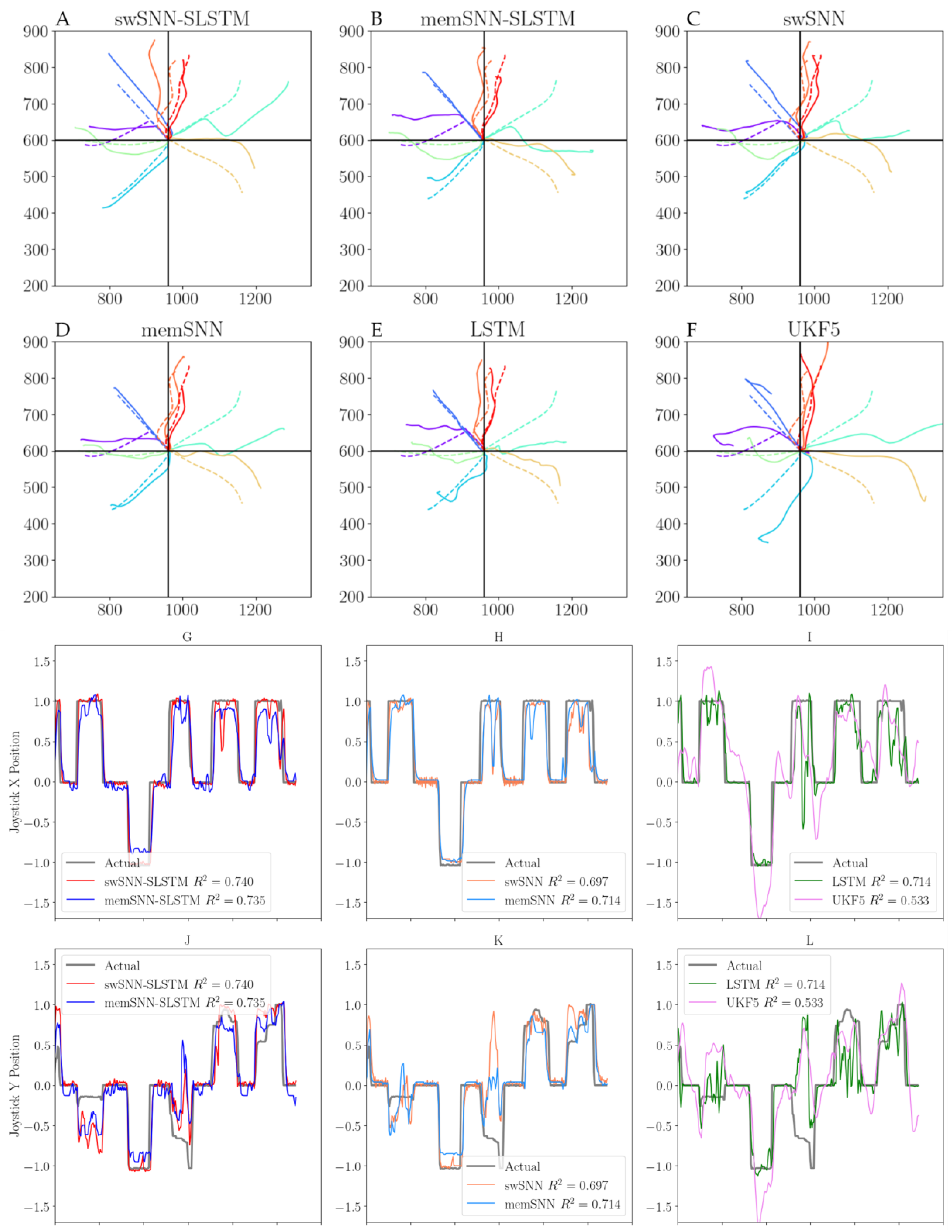
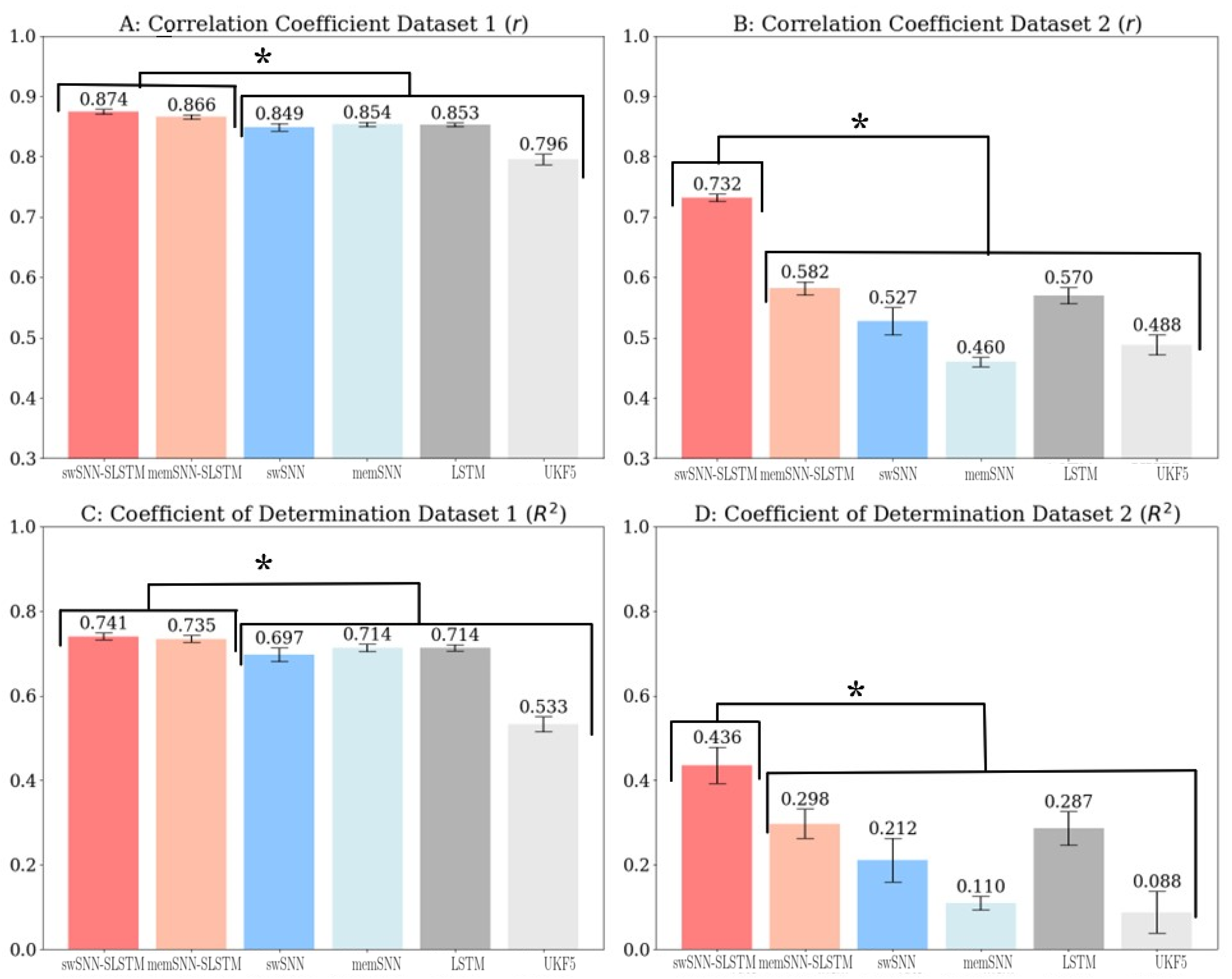
To evaluate the performance of a decoder on a given dataset, we performed 5-fold cross-validation, using 80% of the dataset to train the decoder and the remaining 20% to evaluate the decoder’s performance, while ensuring that the training set did not overlap with the validation set.

Decoded values were evaluated using two metrics: the Pearson correlation coefficient (r) and the coefficient of determination ($R^2$). The correlation coefficient was calculated as follows:

$$r_{x,y}=\frac{cov\left(x,y\right)}{{\mathrm{\sigma }}_x{\mathrm{\sigma }}_y}$$

While the coefficient of determination was calculated as follows:

$$R^2=1-\frac{{{\displaystyle \sum }}_i{\left(x_i-y_i\right)}^2}{{{\displaystyle \sum }}_i{\left(x_i-\overline{x}\right)}^2}$$

where $x$ is the actual kinematic variable at time $i,$ $y$ is the decode kinematic variable, $\mathrm{cov}$ is the covariance and $\mathrm{\sigma }$ is the standard deviation.

The $\mathrm{\alpha }$ values were corrected by Bonferroni’s correction $\mathrm{\alpha }/\mathrm{n}$, where n is number of tests and $\mathrm{\alpha }$ is the significance level.

3. Results

We trained and tested a variety of ML models on our two datasets. In this section, we will describe our findings of how the different models performed in comparison with each other, how variations in model architecture affected decoding accuracy, and how the different models required different numbers of operations to function. Where not otherwise stated, p-values were obtained by performing t-tests.

3.1. Decoder Analysis

For Dataset 1, we evaluated how well our decoders produced joystick trajectories, using the correlation coefficient between actual trajectories and decoded trajectories as a metric of model accuracy. Using two-tailed t-tests, we found that both SLSTM models perform significantly better ($p<5\times {10}^{-3}$) than all other decoders. However, the two SLSTM models did not perform significantly differently when compared to one another (p = 0.122).

When we compared the LSTM model with the spiking neural networks without (S)LSTM layers, they all performed similarly ($p>0.2$). However, all performed much better than the unscented Kalman filter ($p<5\times {10}^{-4}$).

The coefficient of determination was then used to analyze the decoding performance. This metric also accounts for absolute errors in the decoded value. For Dataset 1, when using a two-tailed t-test, we again found that the swSNN-SLSTM and memSNN-SLSTM were statistically similar ($p=0.59$), while outperforming ($p<0.01$) all other decoders. Again, the non-SLSTM layer spiking neural networks and the LSTM neural network performed similarly ($p>0.34$), but significantly outperformed the Kalman filter ($p<1\times {10}^{-5}$).

Figure 2 shows plots of eight successful trials from Dataset 1, decoded by each of the six decoding algorithms used. swSNN-SLSTM and memSNN-SLSTM displayed a comparable performance, with the decoded trajectories closely matching the ground truth, which is the actual joystick position. However, those decoded using swSNN-SLSTM overshoot by a small amount, while memSNN-SLSTM varies, both overshooting and undershooting. We can also see that swSNN, memSNN, and the LSTM decoder display a worse tracking of decoder performance. We can also clearly see that the main problem with the UKF5 Kalman filter is that it frequently overshot and undershot when the ground truth encountered a sudden change.

When we looked at the actual joystick trajectories for Dataset 1, we noticed specific issues with some of the decoders. For the spike-weighted SNNs, we observed that swSNN displayed oscillatory behavior when the joystick position remained at 0. However, this issue was reduced for the swSNN-SLSTM decoder.

The membrane-based SNN, memSNN, did not have large changes in its gradient when rising or falling. However, it did not fall to 0 when the joystick was at rest. memSNN-SLSTM also did not fall to 0 as cleanly as swSNN-SLSTM; however, it improved when compared to memSNN. On the other hand, the LSTM model was able to settle at 0, but showed a worse tracking of peaks and troughs in joystick movements.

We can also quantify model performance by looking at the correlation coefficients and coefficients of determination for the decoded position variables (Figure 3). Using two-tailed t-tests, we can see that swSNN-SLSTM outperforms all other decoders ($p<5\times {10}^{-5}$). We also found that memSNN-SLSTM, and LSTM performed statistically similarly (p = 0.50); however, they also outperformed the SNN models and UKF5 (p < 0.01). swSNN’s performance was statistically similar to both memSNN and the Kalman filter (p > 0.05).

Regarding the coefficient of determination for Dataset 2, we found that swSNN-SLSTM statistically outperforms ($p<0.05$) all other decoders. The memSNN-SLSTM and LSTM model performed statistically similarly (p = 0.84) and performed similarly to swSNN (p = 0.178). They outperformed memSNN and UKF5 (p < 0.05). swSNN, memSNN, and UKF5 all performed similarly (p > 0.113).

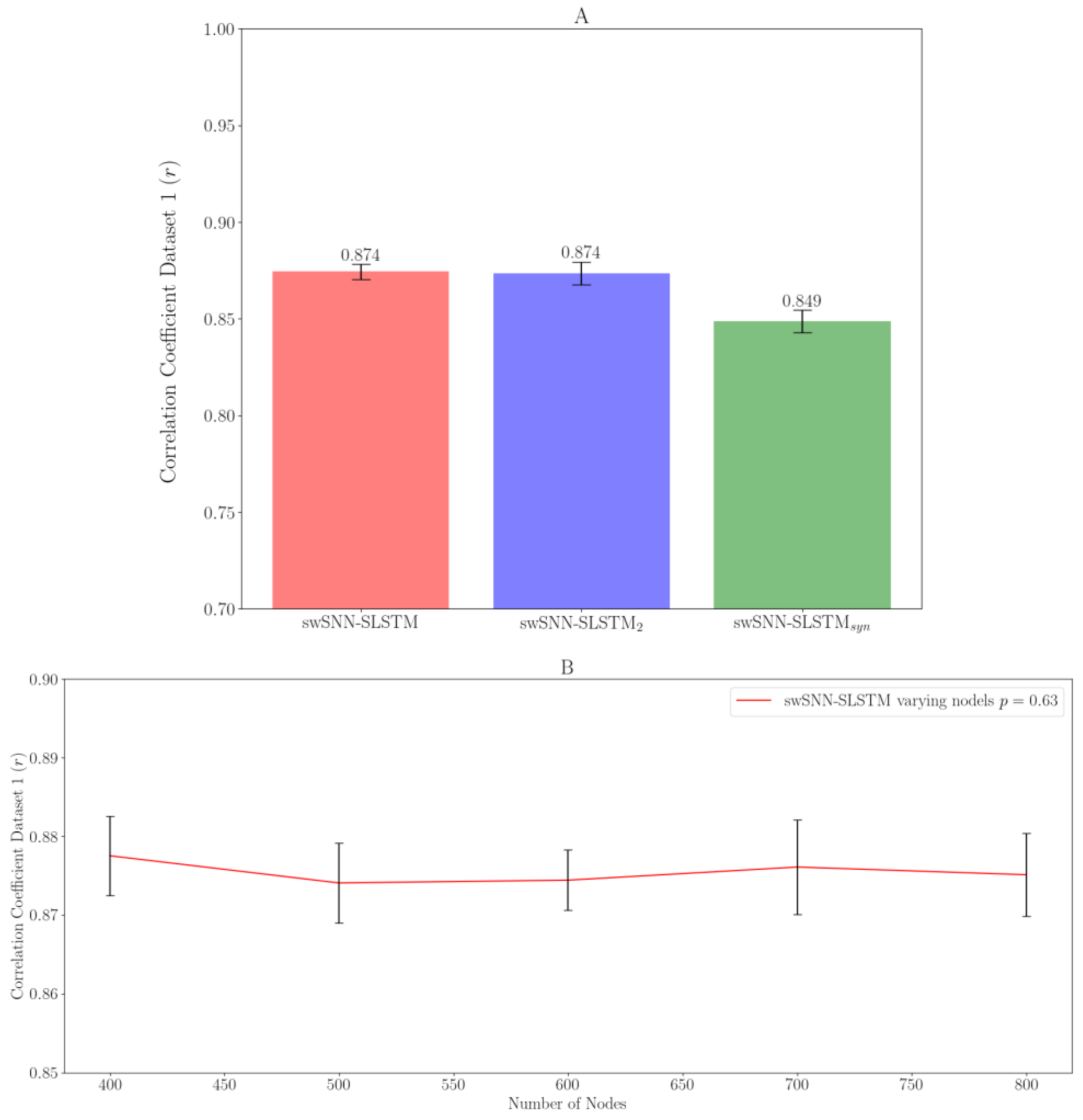
3.2. Variations of SLSTM Architecture

For swSNN-SLSTM₂, we added a second SLSTM layer after the first SLSTM layer, and for swSNN-SLSTM_syn, we replaced the LIF neurons with the synaptic LIF neurons. When we made these adjustments, swSNN-SLSTM₂ had a mean $\mathrm{r}=0.874$ and swSNN-SLSTM_syn had a mean $\mathrm{r}=0.849$ (Figure 4A). We found that increasing the SLSTM layers by one has a negligible impact ($p>0.90$); however, the synthetic neuron model has a much lower correlation coefficient that is significantly significant ($p<5\times {10}^{-3}$).

We also varied the number of output nodes. After making these adjustments, we can see they have no significant impact on the performance of the decoder. p = 0.63 and the mean = 0.878, 0.874, 0.874, 0.876, and 0.875 for 400, 500, 600, 700, and 800 output nodes, respectively (Figure 4B).

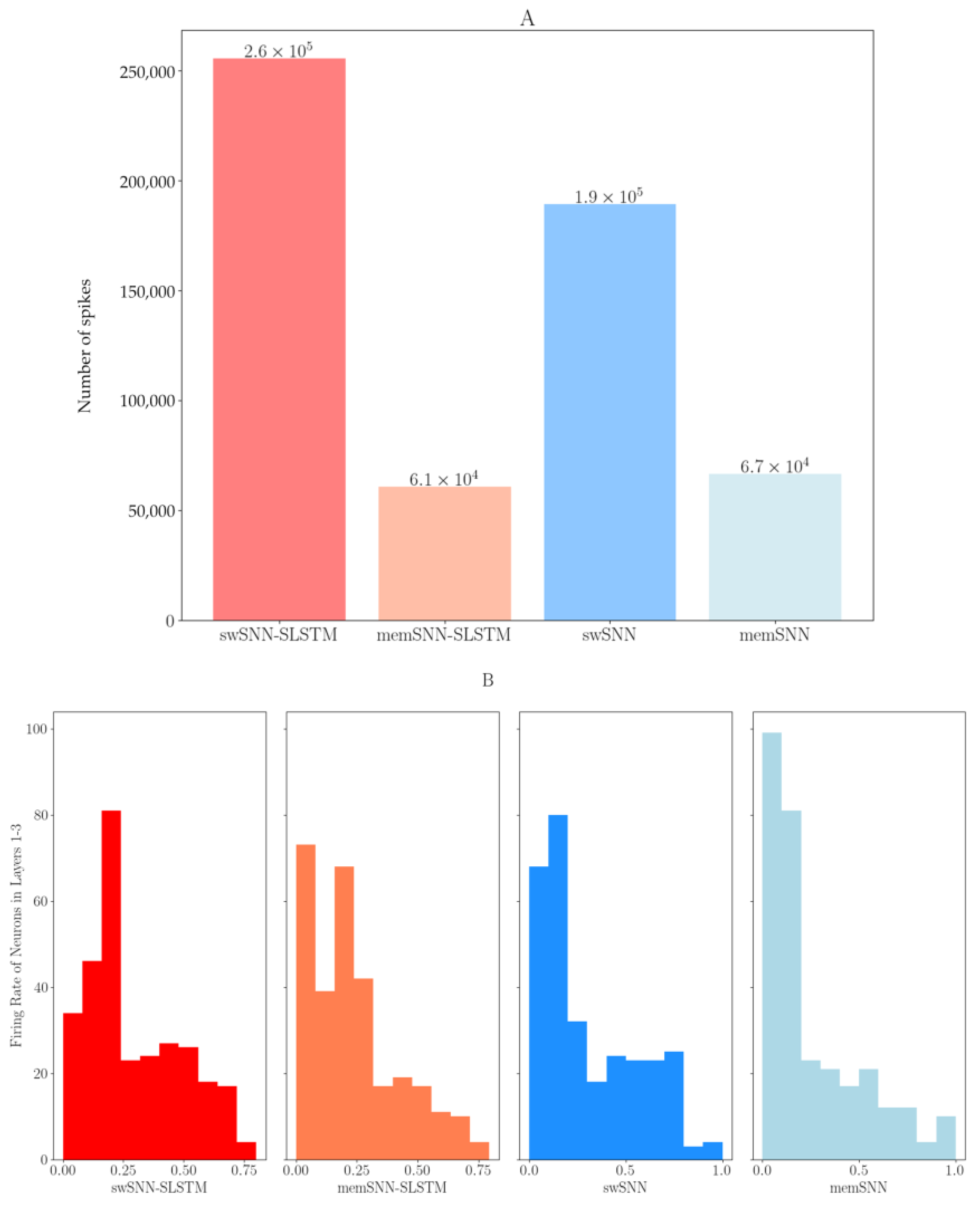
3.3. Firing Rate Analysis

SNNs have the potential to be more efficient than traditional ANNs [45], and the way they can achieve this is through the sparsity of (virtual) neurons that are firing. Fewer neurons firing means a lower number of calculations are required to train and run the models.

In non-spiking ANNs, each neuron’s weight calculation requires a Multiply and Accumulate (MAC) calculation operation per input. In LSTM layers, four MAC calculations are required [46]. In SNNs, however, the output is either a 0 or 1 instead of a floating-point representation. This means only one addition operation [27] is required. In SLSTM layers, again, this is reduced to four addition (ADD) operations. However, SNNs must also update their membrane potential with each step, which, as a floating-point variable, requires one MAC operation per neuron. Each SLSTM layer also has a synaptic membrane potential, which requires two MAC calculations. Using a conservative estimate of three ADD to one MAC operation according to the ratio of energy in [47], we can estimate the cost of operations for a forward pass.

The Unscented Kalman Filter’s complexity is outlined in [48] and each measurement update requires 8/3L³ + 12NL² + 2N²L + 6L² + 10NL + N² + 19/3L + N floating point operations (FLOP) per measurement update, where L is the number of parameters and N is the sigma points. This leads to 3.48 × 10⁷ FLOP. Since two FLOPs equal about one MAC, this is 1.74 × 10⁷ MAC operations.

For an input of 872 timesteps,

Table 2. Table of forward pass operations.

Models	LIF Spikes	SLSTM Spikes	MAC	ADD	Total Operations
UKF5	0	0	1.74 × 107	0	1.74 × 107
LSTM	0	0	5.25 × 105	0	5.25 × 105
swSNN	1.89 × 105	0	900	1.89 × 105	6.4 × 104
memSNN	6.7 × 104	0	300	6.7 × 104	2.7 × 104
swSNN-SLSTM	2.4 × 105	1.4 × 104	1000	2.96 × 105	1.0 × 105
memSNN-SLSTM	5.3 × 104	1.4 × 104	400	1.09 × 105	3.7 × 104

indicates the number of operations required.

In Figure 5A, we can clearly see that all SNN and SLSTM models require fewer total operations than the LSTM model and the membrane-based models require significantly less operations, mainly due to the fact they do not require the output 600 spike layer. We can also see that the forward pass of the UKF5 requires more calculations and takes a lot more time to run; however, there is practically no training time for the UKF5.

Figure 5B shows the firing rate of neurons in layers 1–3, the layers directly preceding the output. It shows that the majority of neurons fire very sparsely.

4. Discussion

We developed a modified spiking neural net implementation of current state-of-the-art movement decoders for a BMI. We find that, for input temporal spiking data, SNNs and SLSTMs perform as well or even better than current state of the art models.

When comparing the SLSTM models, we found that they performed statistically better than their equivalent SNN models. This is an expected result, as SLSTM models are able to capture the temporal dynamics of neuronal activity, which non-recurrent SNNs cannot. Even the LSTM (which is a recurrent classical neural network) slightly underperformed when compared to the two SLSTMs in Dataset 1 and performed far worse than the two SLSTMs in Dataset 2 (Figure 3), showing that spiking neural networks can provide much better decoders for spiking temporal data than classical neural networks in BMI applications. What is even more surprising is the fact that the SNNs also performed similarly to the LSTM model, especially in Dataset 1, and swSNN in Dataset 2. However, this could be explained by the fact that the membrane potential also offers some form of ‘memory’, as it is updated every time step from the previous timestep, so perhaps SNNs without SLSTMs can capture some temporal information, even if it is not as accurate.

When we look at the differences between Dataset 1 and Dataset 2, we find that the Spike-weight based models and membrane-based models performed very differently for each dataset. In Dataset 1, the membrane-based SNN offered a slight performance increase compared to the spike-weight-based SNN; however, in Dataset 2, the spike-weight-based models performed significantly better. It is possible that the performance of spike-weight- and membrane-based SNNs may be dependent on the specific dataset used, and that both have their roles in BMI development. In Dataset 1, the joystick position can be both negative and positive, but for Dataset 2, the x and y positions of a finger were only positive. Further investigation should be carried out to further explore what specific applications both methods are best suited to, and what further modifications can be made. For example, how should negative input values be translated into spikes? Another possible improvement would be not using the same spike weighting for each variable. Figure 2 illustrates that the y position predictions are worse than the x position predictions. Perhaps the spike weighting for the y variable could be adjusted or the number of nodes representing only the y position could be changed. One other possibility is that models with a sparsity of spikes could be encouraged by using a non-linear encoding scheme that encodes common values using a lower number of spikes.

We found that neural networks achieve a much better performance than Kalman filters, probably due to their ability to capture non-linearities within the input data. They are much less likely to overshoot joystick position in places where the joystick remains stationary, and while several studies have attempted to solve this issue in Kalman filters [11,49] through additional add-ons, none of the ANNs require these additions.

We further investigated alternative swSNN-SLSTM architectures. Firstly, replacing the LIF neurons with synaptic neurons made the model much worse. One possible reason for this is that SNNs have problems with local minima [50] and increasing the number of trainable parameters increases the dimensionality, leading to more local minima, which can make it harder for the model to train.

On the other hand, the hyperparameter optimization options we explored, such as adding an extra SLSTM layer or changing the number of nodes in the output layer, had no noticeable effect. This is especially surprising regarding the number of nodes used, as more nodes should lead to more information flow and higher precision. However, it could be that, when the resolution of the data is not increased, changing the number of nodes has little effect. This is a typical problem in the understanding of neural network architecture: it is difficult to understand what each layer is doing or to predict how changes to the architecture will affect performance due to the black box nature of neural networks [51].

When examining firing rates during testing, the proposed SLSTM and SNN models require much fewer operations with respect to traditional neural networks. The membrane models also offer better computational efficiency as they do not require the output 600 spike layer. This could offer significant performance advantages compared to low-power systems and neuromorphic hardware, which is able to take advantage of this fact and could lead to a much more efficient forward pass. It may also be beneficial for devices implanted in the brain, as better computational efficiency leads to lower electricity usage and lower thermal output; elevated temperatures can easily cause harm to neural tissue.

Another observation we made is that most of the neurons fire very rarely, while a small number of neurons fire most of the time (and potentially transfer most of the information). It appears that the SNNs train themselves for sparse coding, where a few neurons send the majority of the information. This is slightly surprising, as a dropout layer was included after every layer. However, this is comparable to real brain activity, as it has been shown that there is sparse coding of information in the brain. This has been shown in brain computer interfaces [52] and physiological recordings from sensory neurons [53]. We can therefore assume that SNNs can provide a reasonable approximation of real biological neurons.

However, despite these performance increases, the SNN and SLSTM models suffer from a key disadvantage. During training, neurons will be updated if they receive a spike. This means it can take a while for a network to develop from its initial state into the final trained sparse state, which requires fewer calculations. Moreover, due to the sequential nature of spiking neural networks, they take far longer to train than the traditional models. The LSTM model took about 5 min to train; however, the SLSTM models both took over 40 min to train. It is likely that devices which have the required memory to train traditional neural networks will nearly always be faster to train than spiking models. This is because most modern-day CPUs and GPUs are optimized for floating point operations. As an alternative to contemporary CPUs and GPUs, biomimetic neuromorphic chips could be used instead to speed up the training process for SNN and SLSTMs. Alternatively, recent research suggests that biomimetic hardware can go even further in the form of brain organoids [54].

Moreover, each spiking model had at least 30 neurons that were ‘dead’ (never firing). This can lead to a constrained information flow between layers and, effectively, these neurons can use up memory and require calculations while never sending any spikes to the next layer in the neural network. However, optimizing for this and reducing the number of nodes in a layer during hyperparameter setting to get rid of these ‘dead’ neurons can lead to problems, as different sets of data require different numbers of neurons to be removed.

In order to improve the models, it is likely that a variable threshold should be added to these ‘dead’ neurons, so their parameters can be updated and they can be removed from calculations during the forward pass. Further tests could be conducted to determine whether removing many neurons, and only keeping those with a high firing rate, would have a negligible impact on the performance of the network while significantly improving memory usage. Alternatively, since the SNNs have no real-world representation of kinematics, they could be used in combination with a Kalman filter, as has been demonstrated in traditional neural networks, as shown in [55].

Overall, our study showed that spiking neural networks can effectively outperform traditional neural networks for use in BMI, where they are decode temporally varying spiking data collected from the motor cortex during the execution of a directional motor task. Since spiking neural networks more accurately model brain neurons than the ‘neurons’ in traditional ANNs, they may be better able to emulate the computations that occur in the brain. The sparsity of spikes that are produced can lead to an efficiency increase in neuromorphic hardware. Given the accuracy of the spike-weighted SLSTM models, we propose that these models can be applied to future BMI devices that are dependent on low-power hardware, especially neuromorphic chips.

In summary, we propose a novel spike-weighted SNN with spiking long short-term memory (swSNN-SLSTM) for brain–machine interfaces (BMIs). Adding SLSTM to spike neural networks can capture temporal information hidden in brain signals. Comparing the proposed algorithm with several existing ML models, the swSNN-SLSTM outperformed both the unscented Kalman filter and the LSTM-based ANN.

References

1. Aggarwal, V.; Mollazadeh, M.; Davidson, A.G.; Schieber, M.H.; Thakor, N.V. State-Based Decoding of Hand and Finger Kinematics Using Neuronal Ensemble and LFP Activity during Dexterous Reach-to-Grasp Movements. J. Neurophysiol. 2013, 109, 3067–3081. [Google Scholar] [CrossRef]
2. Carmena, J.M.; Lebedev, M.A.; Crist, R.E.; O’Doherty, J.E.; Santucci, D.M.; Dimitrov, D.F.; Patil, P.G.; Henriquez, C.S.; Nicolelis, M.A.L. Learning to Control a Brain–Machine Interface for Reaching and Grasping by Primates. PLoS Biol. 2003, 1, e42. [Google Scholar] [CrossRef]
3. So, R.; Xu, Z.; Libedinsky, C.; Toe, K.K.; Ang, K.K.; Yen, S.-C.; Guan, C. Neural Representations of Movement Intentions during Brain-Controlled Self-Motion. In Proceedings of the 2015 7th International IEEE/EMBS Conference on Neural Engineering (NER), Montpellier, France, 22–24 April 2015; pp. 228–231. [Google Scholar]
4. Nason-Tomaszewski, S.R.; Mender, M.J.; Kennedy, E.; Lambrecht, J.M.; Kilgore, K.L.; Chiravuri, S.; Kumar, N.G.; Kung, T.A.; Willsey, M.S.; Chestek, C.A.; et al. Restoring Continuous Finger Function with Temporarily Paralyzed Nonhuman Primates Using Brain–Machine Interfaces. J. Neural Eng. 2023, 20, 036006. [Google Scholar] [CrossRef]
5. Brandman, D.M.; Hosman, T.; Saab, J.; Burkhart, M.C.; Shanahan, B.E.; Ciancibello, J.G.; Sarma, A.A.; Milstein, D.J.; Vargas-Irwin, C.E.; Franco, B.; et al. Rapid Calibration of an Intracortical Brain–Computer Interface for People with Tetraplegia. J. Neural Eng. 2018, 15, 026007. [Google Scholar] [CrossRef] [PubMed]
6. Soekadar, S.R.; Birbaumer, N.; Slutzky, M.W.; Cohen, L.G. Brain–Machine Interfaces in Neurorehabilitation of Stroke. Neurobiol. Dis. 2015, 83, 172–179. [Google Scholar] [CrossRef]
7. Kalman, R.E. A New Approach to Linear Filtering and Prediction Problems. J. Basic Eng. 1960, 82, 35–45. [Google Scholar] [CrossRef]
8. Chen, Z.; Takahashi, K. Sparse Bayesian Inference Methods for Decoding 3D Reach and Grasp Kinematics and Joint Angles with Primary Motor Cortical Ensembles. In Proceedings of the 2013 35th Annual International Conference of the IEEE Engineering in Medicine and Biology Society (EMBC), Osaka, Japan, 3–7 July 2013; pp. 5930–5933. [Google Scholar]
9. Li, Z.; O’Doherty, J.E.; Hanson, T.L.; Lebedev, M.A.; Henriquez, C.S.; Nicolelis, M.A.L. Unscented Kalman Filter for Brain-Machine Interfaces. PLoS ONE 2009, 4, e6243. [Google Scholar] [CrossRef] [PubMed]
10. Dangi, S.; Gowda, S.; Héliot, R.; Carmena, J.M. Adaptive Kalman Filtering for Closed-Loop Brain-Machine Interface Systems. In Proceedings of the 2011 5th International IEEE/EMBS Conference on Neural Engineering, Cancun, Mexico, 27 April–1 May 2011; pp. 609–612. [Google Scholar]
11. Homer, M.L.; Harrison, M.T.; Black, M.J.; Perge, J.A.; Cash, S.S.; Friehs, G.; Hochberg, L.R. Mixing Decoded Cursor Velocity and Position from an Offline Kalman Filter Improves Cursor Control in People with Tetraplegia. In Proceedings of the 2013 6th International IEEE/EMBS Conference on Neural Engineering (NER), San Diego, CA, USA, 6–8 November 2013; pp. 715–718. [Google Scholar]
12. Maksimenko, V.A.; Frolov, N.S.; Hramov, A.E.; Runnova, A.E.; Grubov, V.V.; Kurths, J.; Pisarchik, A.N. Neural Interactions in a Spatially-Distributed Cortical Network During Perceptual Decision-Making. Front. Behav. Neurosci. 2019, 13, 220. [Google Scholar] [CrossRef] [PubMed]
13. Li, S.; Li, J.; Li, Z. An Improved Unscented Kalman Filter Based Decoder for Cortical Brain-Machine Interfaces. Front. Neurosci. 2016, 10, 587. [Google Scholar] [CrossRef] [PubMed]
14. Tseng, P.-H.; Urpi, N.A.; Lebedev, M.; Nicolelis, M. Decoding Movements from Cortical Ensemble Activity Using a Long Short-Term Memory Recurrent Network. Neural Comput. 2019, 31, 1085–1113. [Google Scholar] [CrossRef]
15. Hosman, T.; Vilela, M.; Milstein, D.; Kelemen, J.N.; Brandman, D.M.; Hochberg, L.R.; Simeral, J.D. BCI Decoder Performance Comparison of an LSTM Recurrent Neural Network and a Kalman Filter in Retrospective Simulation. In Proceedings of the 2019 9th International IEEE/EMBS Conference on Neural Engineering (NER), San Francisco, CA, USA, 20–23 March 2019; pp. 1066–1071. [Google Scholar]
16. Premchand, B.; Toe, K.K.; Wang, C.; Shaikh, S.; Libedinsky, C.; Ang, K.K.; So, R.Q. Decoding Movement Direction from Cortical Microelectrode Recordings Using an LSTM-Based Neural Network. In Proceedings of the 2020 42nd Annual International Conference of the IEEE Engineering in Medicine & Biology Society (EMBC), Montreal, QC, Canada, 20–24 July 2020; pp. 3007–3010. [Google Scholar]
17. Konstantakos, V.; Chatzigeorgiou, A.; Nikolaidis, S.; Laopoulos, T. Energy Consumption Estimation in Embedded Systems. Instrum. Meas. IEEE Trans. 2008, 57, 797–804. [Google Scholar] [CrossRef]
18. Sze, V.; Chen, Y.-H.; Yang, T.-J.; Emer, J.S. Efficient Processing of Deep Neural Networks: A Tutorial and Survey. Proc. IEEE 2017, 105, 2295–2329. [Google Scholar] [CrossRef]
19. Wolf, P.D. Thermal Considerations for the Design of an Implanted Cortical Brain–Machine Interface (BMI). In Indwelling Neural Implants: Strategies for Contending with the In Vivo Environment; Reichert, W.M., Ed.; Frontiers in Neuroengineering; CRC Press/Taylor & Francis: Boca Raton, FL, USA, 2008; ISBN 978-0-8493-9362-4. [Google Scholar]
20. Ghosh-Dastidar, S.; Adeli, H. Spiking Neural Networks. Int. J. Neural Syst. 2009, 19, 295–308. [Google Scholar] [CrossRef] [PubMed]
21. van Schaik, A. Building Blocks for Electronic Spiking Neural Networks. Neural Netw. 2001, 14, 617–628. [Google Scholar] [CrossRef] [PubMed]
22. Han, B.; Sengupta, A.; Roy, K. On the Energy Benefits of Spiking Deep Neural Networks: A Case Study. In Proceedings of the 2016 International Joint Conference on Neural Networks (IJCNN), Vancouver, BC, Canada, 24–29 July 2016; pp. 971–976. [Google Scholar]
23. Henkes, A.; Eshraghian, J.K.; Wessels, H. Spiking Neural Networks for Nonlinear Regression. arXiv 2022, arXiv:2210.03515. [Google Scholar]
24. Sorbaro, M.; Liu, Q.; Bortone, M.; Sheik, S. Optimizing the Energy Consumption of Spiking Neural Networks for Neuromorphic Applications. Front. Neurosci. 2020, 14, 662. [Google Scholar] [CrossRef] [PubMed]
25. Wu, Y.; Deng, L.; Li, G.; Zhu, J.; Shi, L. Spatio-Temporal Backpropagation for Training High-Performance Spiking Neural Networks. Front. Neurosci. 2018, 12, 331. [Google Scholar] [CrossRef] [PubMed]
26. Iakymchuk, T.; Rosado-Muñoz, A.; Guerrero-Martínez, J.F.; Bataller-Mompeán, M.; Francés-Víllora, J.V. Simplified Spiking Neural Network Architecture and STDP Learning Algorithm Applied to Image Classification. EURASIP J. Image Video Process. 2015, 2015, 4. [Google Scholar] [CrossRef]
27. Liao, J.; Widmer, L.; Wang, X.; Di Mauro, A.; Nason-Tomaszewski, S.R.; Chestek, C.A.; Benini, L.; Jang, T. An Energy-Efficient Spiking Neural Network for Finger Velocity Decoding for Implantable Brain-Machine Interface. In Proceedings of the 2022 IEEE 4th International Conference on Artificial Intelligence Circuits and Systems (AICAS), Incheon, Republic of Korea, 13–15 June 2022; pp. 134–137. [Google Scholar]
28. Nason, S.R.; Mender, M.J.; Vaskov, A.K.; Willsey, M.S.; Ganesh Kumar, N.; Kung, T.A.; Patil, P.G.; Chestek, C.A. Example Data and Code for “Real-Time Linear Prediction of Simultaneous and Independent Movements of Two Finger Groups Using an Intracortical Brain-Machine Interface”; University of Michigan: Ann Arbor, MI, USA, 2021. [Google Scholar] [CrossRef]
29. Nason, S.R.; Mender, M.J.; Vaskov, A.K.; Willsey, M.S.; Ganesh Kumar, N.; Kung, T.A.; Patil, P.G.; Chestek, C.A. Real-Time Linear Prediction of Simultaneous and Independent Movements of Two Finger Groups Using an Intracortical Brain-Machine Interface. Neuron 2021, 109, 3164–3177.e8. [Google Scholar] [CrossRef]
30. Libedinsky, C.; So, R.; Xu, Z.; Kyar, T.K.; Ho, D.; Lim, C.; Chan, L.; Chua, Y.; Yao, L.; Cheong, J.H.; et al. Independent Mobility Achieved through a Wireless Brain-Machine Interface. PLoS ONE 2016, 11, e0165773. [Google Scholar] [CrossRef]
31. Yang, H.; Libedinsky, C.; Guan, C.; Ang, K.; So, R. Boosting Performance in Brain-Machine Interface by Classifier-Level Fusion Based on Accumulative Training Models from Multi-Day Data. In Proceedings of the 2017 39th Annual International Conference of the IEEE Engineering in Medicine and Biology Society (EMBC), Jeju, Republic of Korea, 11–15 July 2017; Volume 2017, pp. 1922–1925. [Google Scholar]
32. Premchand, B.; Toe, K.K.; Wang, C.C.; Libedinsky, C.; Ang, K.K.; So, R.Q. Rapid Detection of Inactive Channels during Multi-Unit Intracranial Recordings. In Proceedings of the 2019 IEEE EMBS International Conference on Biomedical & Health Informatics (BHI), Chicago, IL, USA, 19–22 May 2019; pp. 1–4. [Google Scholar]
33. Ludwig, K.A.; Miriani, R.M.; Langhals, N.B.; Joseph, M.D.; Anderson, D.J.; Kipke, D.R. Using a Common Average Reference to Improve Cortical Neuron Recordings From Microelectrode Arrays. J. Neurophysiol. 2009, 101, 1679–1689. [Google Scholar] [CrossRef] [PubMed]
34. Eshraghian, J.K.; Ward, M.; Neftci, E.; Wang, X.; Lenz, G.; Dwivedi, G.; Bennamoun, M.; Jeong, D.S.; Lu, W.D. Training Spiking Neural Networks Using Lessons From Deep Learning. Proc. IEEE 2023, 111, 1016–1054. [Google Scholar] [CrossRef]
35. Rathi, N.; Srinivasan, G.; Panda, P.; Roy, K. Enabling Deep Spiking Neural Networks with Hybrid Conversion and Spike Timing Dependent Backpropagation. arXiv 2020, arXiv:2005.01807. [Google Scholar]
36. Masquelier, T.; Thorpe, S.J. Unsupervised Learning of Visual Features through Spike Timing Dependent Plasticity. PLoS Comput. Biol. 2007, 3, e31. [Google Scholar] [CrossRef]
37. Gers, F.A.; Schmidhuber, J.; Cummins, F. Learning to Forget: Continual Prediction with LSTM. Neural Comput. 2000, 12, 2451–2471. [Google Scholar] [CrossRef] [PubMed]
38. Tan, P.-Y.; Wu, C.-W.; Lu, J.-M. An Improved STBP for Training High-Accuracy and Low-Spike-Count Spiking Neural Networks. In Proceedings of the 2021 Design, Automation & Test in Europe Conference & Exhibition (DATE), Virtual, 1–5 February 2021; pp. 575–580. [Google Scholar]
39. Fang, W.; Yu, Z.; Chen, Y.; Huang, T.; Masquelier, T.; Tian, Y. Deep Residual Learning in Spiking Neural Networks. In Proceedings of the 34th Conference on Advances in Neural Information Processing Systems, Online, 6–14 December 2021; Curran Associates, Inc.: Red Hook, NY, USA, 2021; Volume 34, pp. 21056–21069. [Google Scholar]
40. Hinton, G.E.; Srivastava, N.; Krizhevsky, A.; Sutskever, I.; Salakhutdinov, R.R. Improving Neural Networks by Preventing Co-Adaptation of Feature Detectors. arXiv 2012, arXiv:1207.0580. [Google Scholar]
41. Kingma, D.P.; Ba, J. Adam: A Method for Stochastic Optimization. arXiv 2017, arXiv:1412.6980. [Google Scholar]
42. Ahmadi, N.; Constandinou, T.G.; Bouganis, C.-S. Robust and Accurate Decoding of Hand Kinematics from Entire Spiking Activity Using Deep Learning. J. Neural Eng. 2021, 18, 026011. [Google Scholar] [CrossRef]
43. Gilja, V.; Nuyujukian, P.; Chestek, C.A.; Cunningham, J.P.; Yu, B.M.; Fan, J.M.; Churchland, M.M.; Kaufman, M.T.; Kao, J.C.; Ryu, S.I.; et al. A High-Performance Neural Prosthesis Enabled by Control Algorithm Design. Nat. Neurosci. 2012, 15, 1752–1757. [Google Scholar] [CrossRef]
44. Wu, W.; Black, M.; Gao, Y.; Serruya, M.; Shaikhouni, A.; Donoghue, J.; Bienenstock, E. Neural Decoding of Cursor Motion Using a Kalman Filter. In Advances in Neural Information Processing Systems; MIT Press: Cambridge, MA, USA, 2002; Volume 15. [Google Scholar]
45. Frontiers|Deep Learning with Spiking Neurons: Opportunities and Challenges. Available online: https://www.frontiersin.org/articles/10.3389/fnins.2018.00774/full (accessed on 2 September 2023).
46. Rezk, N.M.; Purnaprajna, M.; Nordström, T.; Ul-Abdin, Z. Recurrent Neural Networks: An Embedded Computing Perspective. IEEE Access 2020, 8, 57967–57996. [Google Scholar] [CrossRef]
47. Horowitz, M. 1.1 Computing’s Energy Problem (and What We Can Do about It). In Proceedings of the 2014 IEEE International Solid-State Circuits Conference Digest of Technical Papers (ISSCC), San Francisco, CA, USA, 9–13 February 2014; pp. 10–14. [Google Scholar]
48. Lü, S.; Zhang, R. Two Efficient Implementation Forms of Unscented Kalman Filter. Control Intell. Syst. 2011, 39, 761–764. [Google Scholar] [CrossRef]
49. Golub, M.D.; Yu, B.M.; Schwartz, A.B.; Chase, S.M. Motor Cortical Control of Movement Speed with Implications for Brain-Machine Interface Control. J. Neurophysiol. 2014, 112, 411–429. [Google Scholar] [CrossRef] [PubMed]
50. Eshraghian, J.K.; Lammie, C.; Azghadi, M.R.; Lu, W.D. Navigating Local Minima in Quantized Spiking Neural Networks. In Proceedings of the 2022 IEEE 4th International Conference on Artificial Intelligence Circuits and Systems (AICAS), Incheon, Republic of Korea, 13–15 June 2022. [Google Scholar]
51. Buhrmester, V.; Münch, D.; Arens, M. Analysis of Explainers of Black Box Deep Neural Networks for Computer Vision: A Survey. arXiv 2019, arXiv:1911.12116. [Google Scholar] [CrossRef]
52. Premchand, B.; Toe, K.K.; Wang, C.; Libedinsky, C.; Ang, K.K.; So, R.Q. Information Sparseness in Cortical Microelectrode Channels While Decoding Movement Direction Using an Artificial Neural Network. In Proceedings of the 2022 44th Annual International Conference of the IEEE Engineering in Medicine & Biology Society (EMBC), Glasgow, UK, 11–15 July 2022; pp. 3534–3537. [Google Scholar]
53. Olshausen, B.; Field, D. Sparse Coding of Sensory Inputs. Curr. Opin. Neurobiol. 2004, 14, 481–487. [Google Scholar] [CrossRef]
54. Cai, H.; Ao, Z.; Tian, C.; Wu, Z.; Liu, H.; Tchieu, J.; Gu, M.; Mackie, K.; Guo, F. Brain Organoid Reservoir Computing for Artificial Intelligence. Nat. Electron. 2023, 6, 1032–1039. [Google Scholar] [CrossRef]
55. Willsey, M.S.; Nason-Tomaszewski, S.R.; Ensel, S.R.; Temmar, H.; Mender, M.J.; Costello, J.T.; Patil, P.G.; Chestek, C.A. Real-Time Brain-Machine Interface in Non-Human Primates Achieves High-Velocity Prosthetic Finger Movements Using a Shallow Feedforward Neural Network Decoder. Nat. Commun. 2022, 13, 6899. [Google Scholar] [CrossRef]
Figure 1. (Left)—architecture is of spike-weighted SNNs; (Right)—architecture of membrane based SNNs and NNs.
Algorithms 17 00156 g001
Figure 2. Top: Two-dimensional joystick cursor positions from Dataset 1. Dashed lines indicate real trajectories, and whole lines indicate decoded trajectories. Each color represents one successful trial (which has one real trajectory and one decoded trajectory). The decoders used are: (A) swSNN-SLSTM; (B) memSNN-SLSTM; (C) swSNN; (D) memSNN; (E) LSTM; (F) UKF5. Bottom: joystick trajectories of decoders in one representative successful trial, separated into x and y dimensions. (G,J) show swSNN-SLSTM and memSNN-SLSTM for x and y, respectively; (H,K) show swSNN and memSNN for x and y, respectively; and (I,L) show LSTM and UKF5 for x and y, respectively.
Algorithms 17 00156 g002
Figure 3. (A) Correlation coefficients for decoders trained and tested on Dataset 1; (B) correlation coefficients for decoders trained and tested on Dataset 2; (C) coefficient of determination for decoders trained and tested on Dataset 1; (D) coefficient of determination for decoders trained and tested on Dataset 2. Asterisks indicate that each category on the higher side significantly outperformed each category on the lower side.
Algorithms 17 00156 g003
Figure 4. (A) Effect of layer variations on the performance of swSNN-SLSTM decoders; (B) performance of swSNN-SLSTM based on number of output nodes.
Algorithms 17 00156 g004
Figure 5. (A) Total number of spikes in various spiking models; (B) firing rate of neurons in layers 1–3.
Algorithms 17 00156 g005