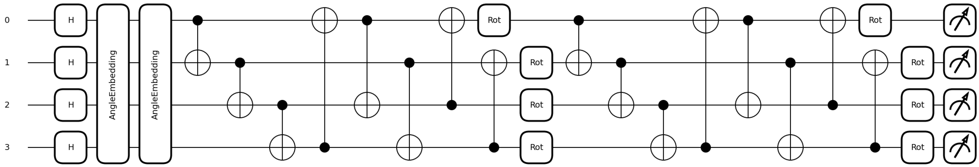
Figure 1.
An example of VQC architecture with two layers of entanglements for QLSTM and QGRU.
Figure 1.
An example of VQC architecture with two layers of entanglements for QLSTM and QGRU.
Figure 2.
Structure of a single unit of classical LSTM.
Figure 2.
Structure of a single unit of classical LSTM.
Figure 3.
Structure of a single unit of classical GRU.
Figure 3.
Structure of a single unit of classical GRU.
Figure 4.
Structure of a single unit of QLSTM.
Figure 4.
Structure of a single unit of QLSTM.
Figure 5.
Structure of a single unit of QGRU.
Figure 5.
Structure of a single unit of QGRU.
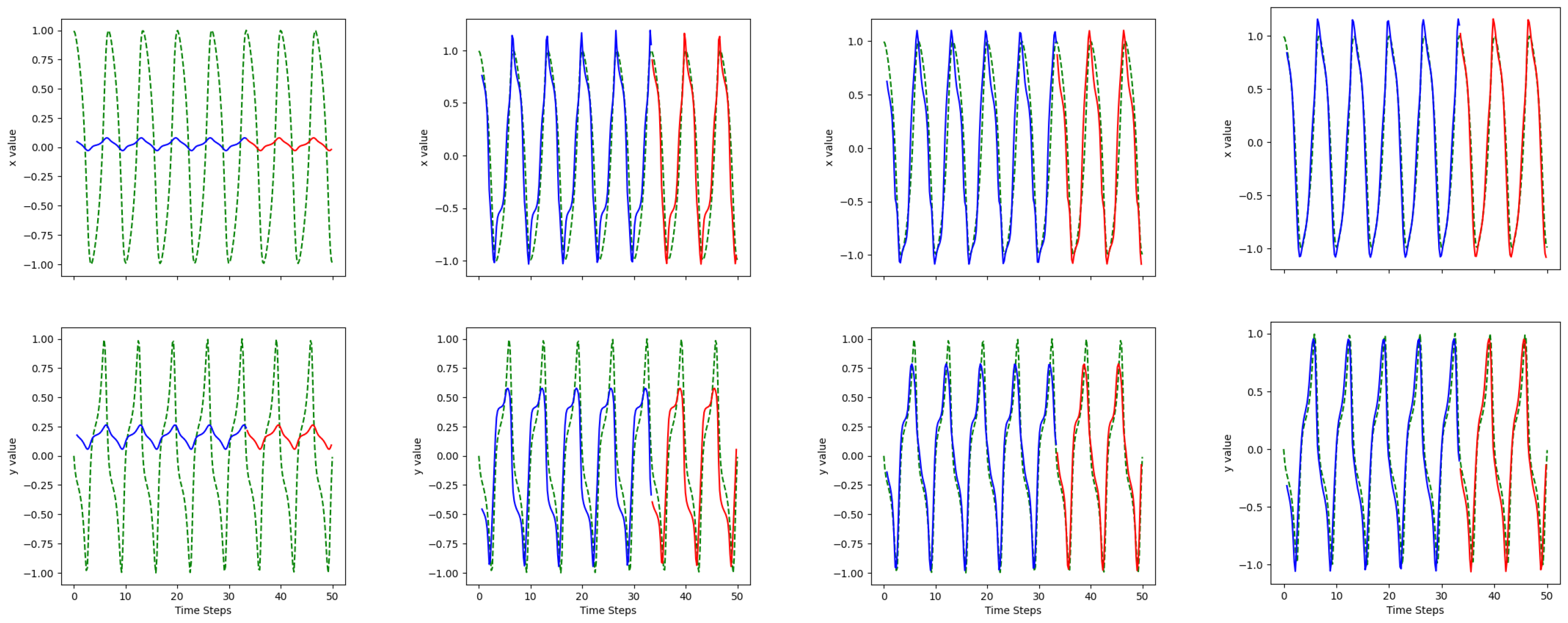
Figure 6.
LSTM predictions over 100 epochs for the Van der Pol oscillator. Up: x; down: y; epoch: 5, 50, 70, 100; green dashed line: actual values; blue solid line: training predictions; red solid line: testing predictions.
Figure 6.
LSTM predictions over 100 epochs for the Van der Pol oscillator. Up: x; down: y; epoch: 5, 50, 70, 100; green dashed line: actual values; blue solid line: training predictions; red solid line: testing predictions.
Figure 7.
QLSTM predictions over 100 Epochs for the Van der Pol oscillator. Up: x; down: y; epoch: 5, 50, 70, 100; green dashed line: actual values; blue solid line: training predictions; red solid line: testing predictions.
Figure 7.
QLSTM predictions over 100 Epochs for the Van der Pol oscillator. Up: x; down: y; epoch: 5, 50, 70, 100; green dashed line: actual values; blue solid line: training predictions; red solid line: testing predictions.
Figure 8.
GRU predictions over 100 Epochs for the Van der Pol oscillator. Up: x; down: y; epoch: 5, 50, 70, 100; green dashed line: actual values; blue solid line: training predictions; red solid line: testing predictions.
Figure 8.
GRU predictions over 100 Epochs for the Van der Pol oscillator. Up: x; down: y; epoch: 5, 50, 70, 100; green dashed line: actual values; blue solid line: training predictions; red solid line: testing predictions.
Figure 9.
QGRU predictions over 100 Epochs for the Van der Pol oscillator. Up: x; down: y; epoch: 5, 50, 70, 100; green dashed line: actual values; blue solid line: training predictions; red solid line: testing predictions.
Figure 9.
QGRU predictions over 100 Epochs for the Van der Pol oscillator. Up: x; down: y; epoch: 5, 50, 70, 100; green dashed line: actual values; blue solid line: training predictions; red solid line: testing predictions.
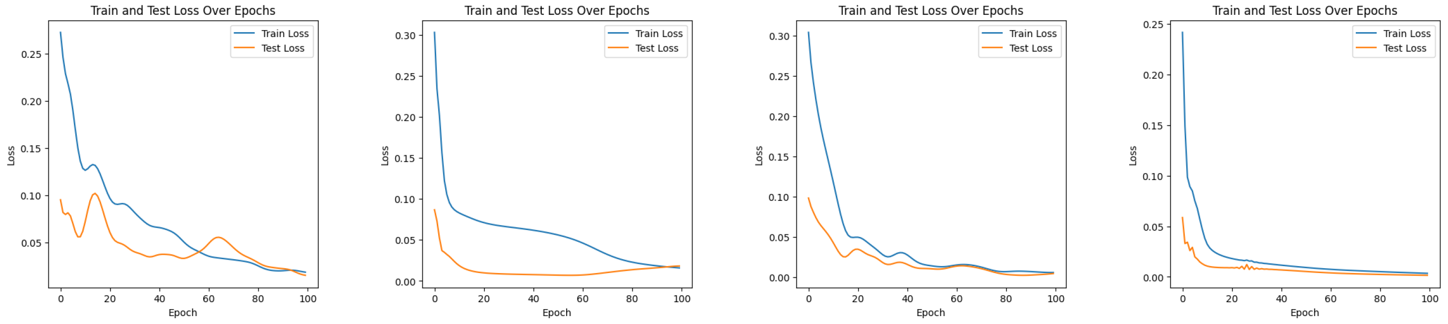
Figure 10.
Experiment 1: Train and test losses for the models over 100 epochs. From left to right: LSTM, QLSTM, GRU, QGRU.
Figure 10.
Experiment 1: Train and test losses for the models over 100 epochs. From left to right: LSTM, QLSTM, GRU, QGRU.
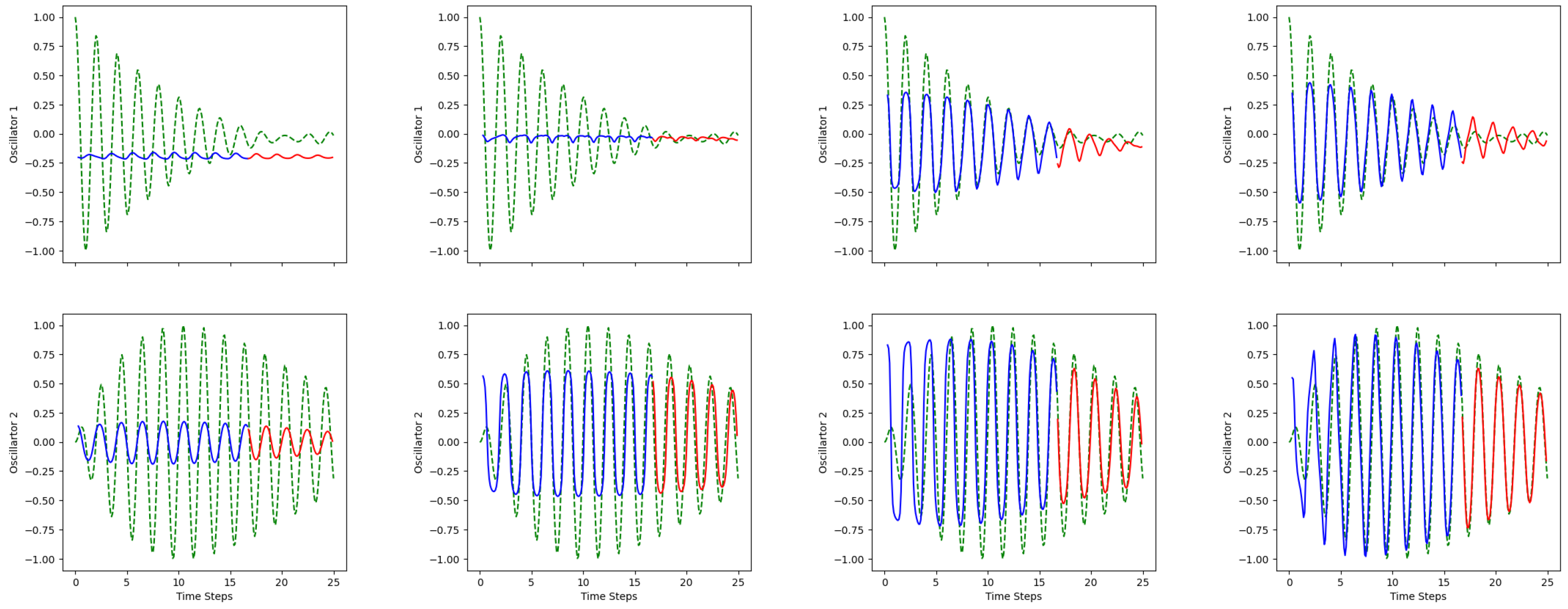
Figure 11.
LSTM predictions over 10 epochs. Up: Oscillator 1; down: Oscillator 2; epoch: 5, 50, 70, 100; green dashed line: actual values; blue solid line: training predictions; red solid line: testing predictions.
Figure 11.
LSTM predictions over 10 epochs. Up: Oscillator 1; down: Oscillator 2; epoch: 5, 50, 70, 100; green dashed line: actual values; blue solid line: training predictions; red solid line: testing predictions.
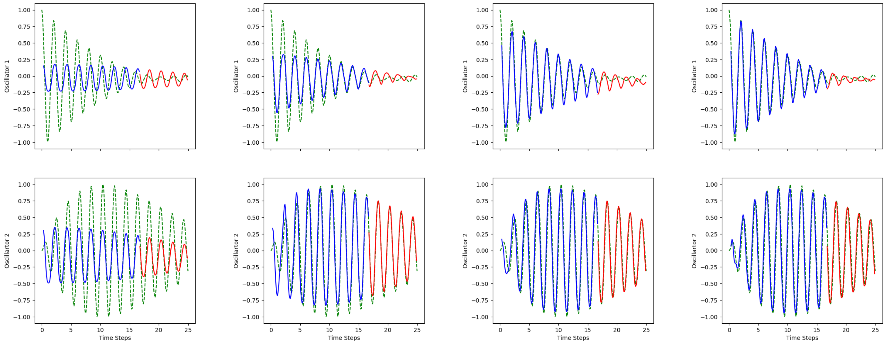
Figure 12.
QLSTM Predictions over 10 epochs. Up: Oscillator 1; down: Oscillator 2; epoch: 5, 50, 70, 100; green dashed line: actual values; blue solid line: training predictions; red solid line: testing predictions.
Figure 12.
QLSTM Predictions over 10 epochs. Up: Oscillator 1; down: Oscillator 2; epoch: 5, 50, 70, 100; green dashed line: actual values; blue solid line: training predictions; red solid line: testing predictions.
Figure 13.
GRU Predictions over 10 epochs. Up: Oscillator 1; down: Oscillator 2; epoch: 5, 50, 70, 100; green dashed line: actual values; blue solid line: training predictions; red solid line: testing predictions.
Figure 13.
GRU Predictions over 10 epochs. Up: Oscillator 1; down: Oscillator 2; epoch: 5, 50, 70, 100; green dashed line: actual values; blue solid line: training predictions; red solid line: testing predictions.
Figure 14.
QGRU Predictions over 10 epochs. Up: Oscillator 1, down: Oscillator 2 epoch: 5, 50, 70, 100; green dashed line: actual values; blue solid line: training predictions; red solid line: testing predictions.
Figure 14.
QGRU Predictions over 10 epochs. Up: Oscillator 1, down: Oscillator 2 epoch: 5, 50, 70, 100; green dashed line: actual values; blue solid line: training predictions; red solid line: testing predictions.
Figure 15.
Experiment 2: train and test losses for the models over 100 epochs. From left to right: LSTM, QLSTM, GRU, QGRU.
Figure 15.
Experiment 2: train and test losses for the models over 100 epochs. From left to right: LSTM, QLSTM, GRU, QGRU.
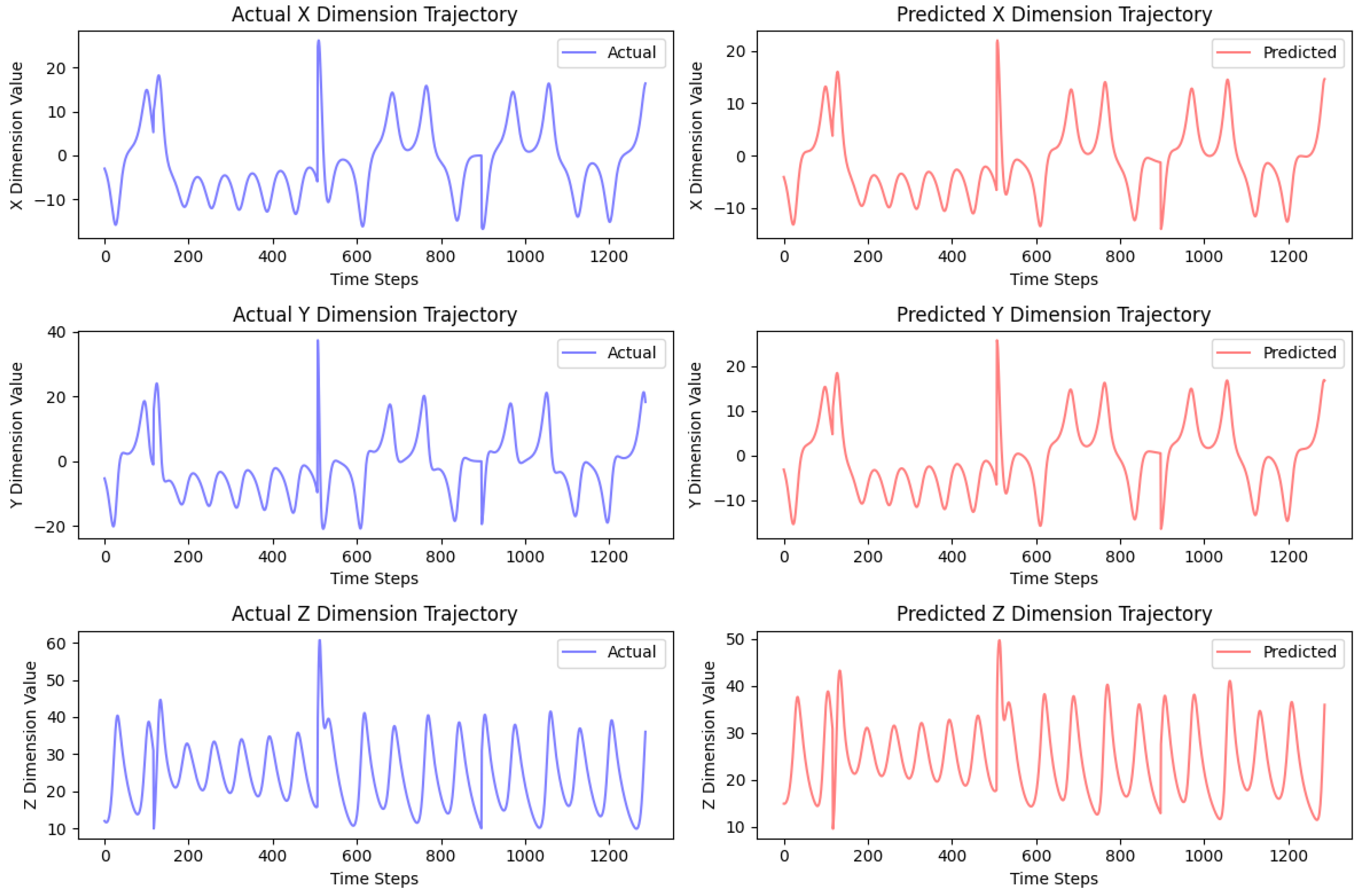
Figure 16.
LSTM predictions for dimensions X (up), Y (middle), and Z (bottom).
Figure 16.
LSTM predictions for dimensions X (up), Y (middle), and Z (bottom).
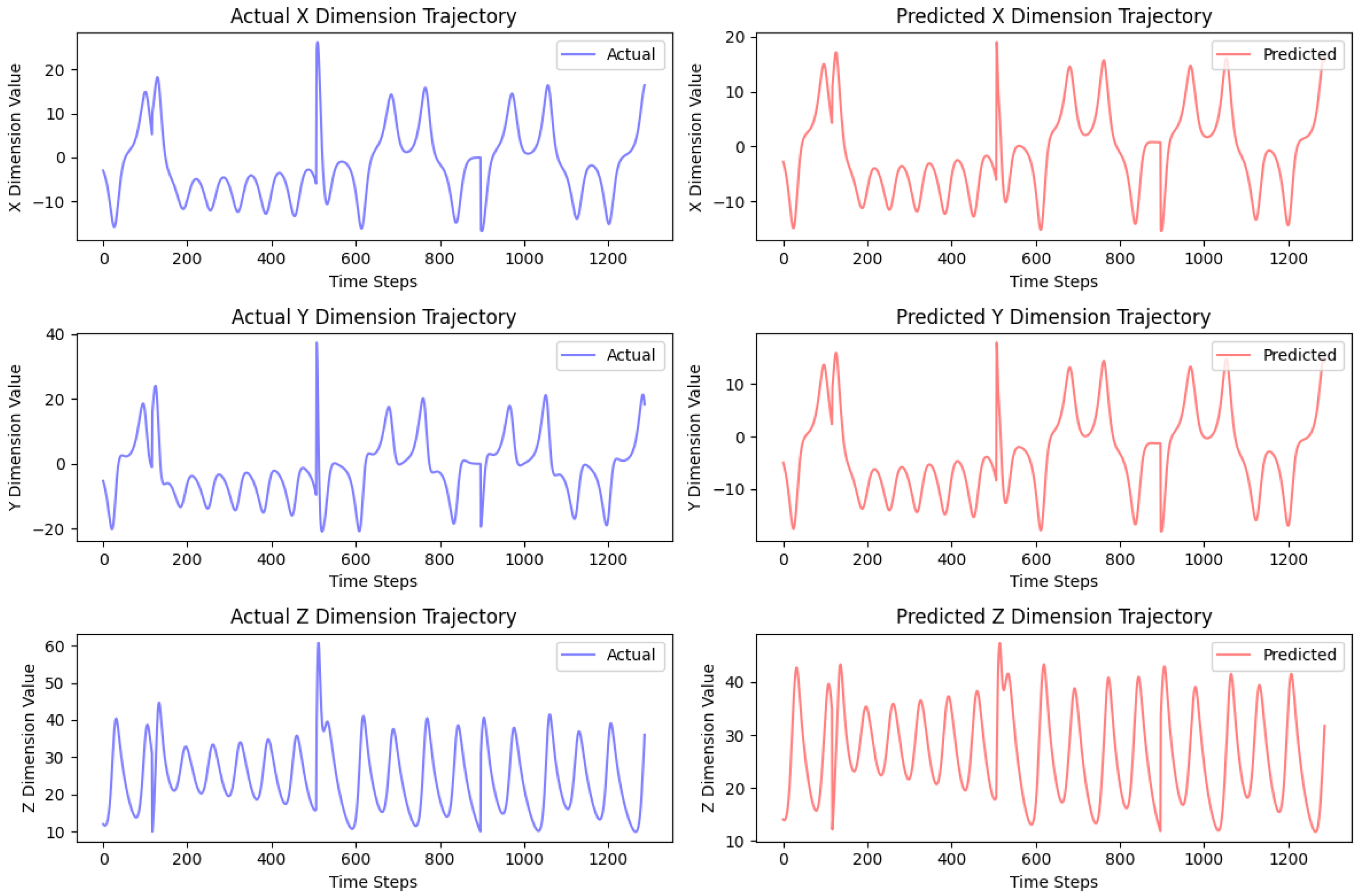
Figure 17.
QLSTM predictions for dimensions X (up), Y (middle), and Z (bottom).
Figure 17.
QLSTM predictions for dimensions X (up), Y (middle), and Z (bottom).
Figure 18.
GRU predictions for dimensions X (up), Y (middle), and Z (bottom).
Figure 18.
GRU predictions for dimensions X (up), Y (middle), and Z (bottom).
Figure 19.
QGRU predictions for dimensions X (up), Y (middle), and Z (bottom).
Figure 19.
QGRU predictions for dimensions X (up), Y (middle), and Z (bottom).
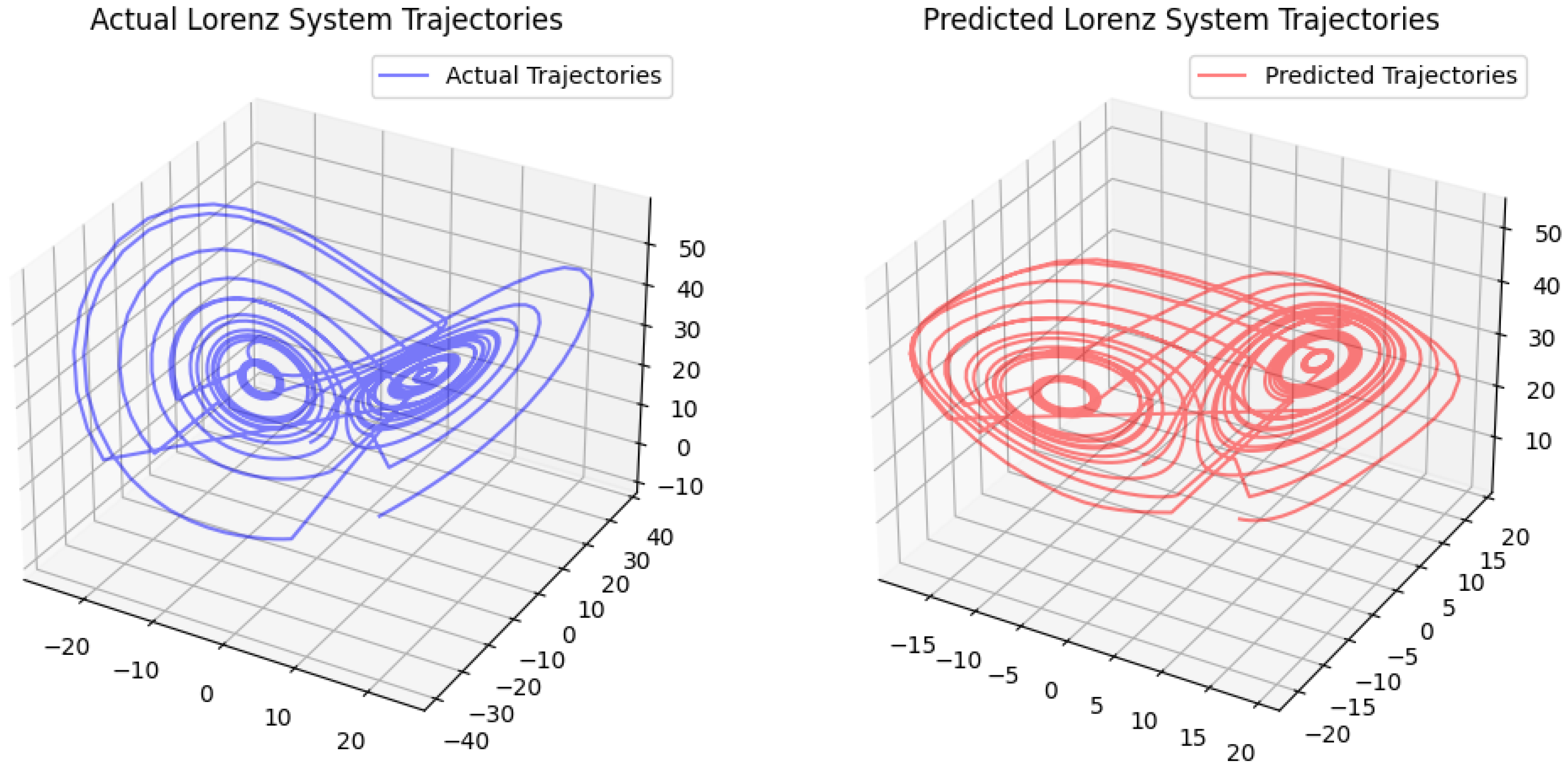
Figure 20.
Predicted Lorenz system trajectory by LSTM model.
Figure 20.
Predicted Lorenz system trajectory by LSTM model.
Figure 21.
Predicted Lorenz system trajectory by QLSTM model.
Figure 21.
Predicted Lorenz system trajectory by QLSTM model.
Figure 22.
Predicted Lorenz system trajectory by GRU model.
Figure 22.
Predicted Lorenz system trajectory by GRU model.
Figure 23.
Predicted Lorenz system trajectory by QGRU model.
Figure 23.
Predicted Lorenz system trajectory by QGRU model.
Figure 24.
Experiment 3: Train and test losses for the models over 20 epochs. From left to right: LSTM, QLSTM, GRU, QGRU.
Figure 24.
Experiment 3: Train and test losses for the models over 20 epochs. From left to right: LSTM, QLSTM, GRU, QGRU.
Table 1.
Hyperparameter configuration.
Table 1.
Hyperparameter configuration.
| Hyperparameter | QRNNs Value | RNNs Value |
|---|
| Optimizer | RMSprop | Adam |
| Loss Function | MSE | MSE |
| Backend | default.qubit | - |
| Number of Qubits | 4 | - |
| Layer of Entanglements | 4 | - |
| Number of Data Points | 250 | 250 |
| Percentage of Train Set | 67% | 67% |
| Percentage of Test Set | 33% | 33% |
| Learning Rate | 0.01 | 0.01 |
Table 2.
Comparison of train and test MAE and RMSE for the state of x.
Table 2.
Comparison of train and test MAE and RMSE for the state of x.
| Model | Train MAE | Test MAE | Train RMSE | Test RMSE |
|---|
| LSTM | 0.2601 | 0.2585 | 0.3002 | 0.2986 |
| QLSTM | 0.1411 | 0.1397 | 0.1648 | 0.1641 |
| GRU | 0.1597 | 0.1591 | 0.1845 | 0.1850 |
| QGRU | 0.0868 | 0.0902 | 0.1013 | 0.1031 |
Table 3.
Comparison of train and test MAE and RMSE for the state of y.
Table 3.
Comparison of train and test MAE and RMSE for the state of y.
| Model | Train MAE | Test MAE | Train RMSE | Test RMSE |
|---|
| LSTM | 0.3224 | 0.3294 | 0.3737 | 0.3828 |
| QLSTM | 0.1959 | 0.1851 | 0.2498 | 0.2384 |
| GRU | 0.3336 | 0.3375 | 0.4319 | 0.4384 |
| QGRU | 0.1473 | 0.1500 | 0.1931 | 0.1943 |
Table 4.
Comparison of train and test MAE and RMSE for Oscillator 1.
Table 4.
Comparison of train and test MAE and RMSE for Oscillator 1.
| Model | Train MAE | Test MAE | Train RMSE | Test RMSE |
|---|
| LSTM | 0.5467 | 0.4371 | 0.7761 | 0.4922 |
| QLSTM | 0.5284 | 0.4763 | 0.6987 | 0.5374 |
| GRU | 0.3648 | 0.4396 | 0.4499 | 0.4941 |
| QGRU | 0.2585 | 0.2411 | 0.3587 | 0.2701 |
Table 5.
Comparison of train and test MAE and RMSE for Oscillator 2.
Table 5.
Comparison of train and test MAE and RMSE for Oscillator 2.
| Model | Train MAE | Test MAE | Train RMSE | Test RMSE |
|---|
| LSTM | 0.2190 | 0.3597 | 0.2814 | 0.4248 |
| QLSTM | 0.1244 | 0.2591 | 0.1607 | 0.2885 |
| GRU | 0.1160 | 0.0858 | 0.1483 | 0.1006 |
| QGRU | 0.0794 | 0.0482 | 0.0949 | 0.0602 |
Table 6.
Hyperparameter configuration for classic models and quantum models.
Table 6.
Hyperparameter configuration for classic models and quantum models.
| Hyperparameter | Quantum | Classic |
|---|
| Optimizer | RMSprop | Adam |
| Loss Function | MSE | MSE |
| Backend | default.qubit | - |
| Number of Qubits | 4 | - |
| VQC Layer | 4 | - |
| Percentage of Train Set | 67% | 67% |
| Percentage of Test Set | 33% | 33% |
| Epochs | 20 | 20 |
| Learning Rate | 0.01 | 0.01 |
Table 7.
Mean Absolute Error (MAE) for each model on test set.
Table 7.
Mean Absolute Error (MAE) for each model on test set.
| Model | X | Y | Z |
|---|
| LSTM | 2.0361 | 2.1232 | 2.2119 |
| QLSTM | 0.8820 | 0.9473 | 1.0206 |
| GRU | 1.1684 | 1.1719 | 1.1710 |
| QGRU | 0.4864 | 0.4723 | 0.4555 |
Table 8.
Root Mean Square Error (RMSE) for each model on test set.
Table 8.
Root Mean Square Error (RMSE) for each model on test set.
| Model | X | Y | Z |
|---|
| LSTM | 2.1736 | 2.2718 | 2.3714 |
| QLSTM | 1.2234 | 1.2723 | 1.3348 |
| GRU | 1.1783 | 1.1748 | 1.1740 |
| QGRU | 0.4971 | 0.4846 | 0.4745 |


