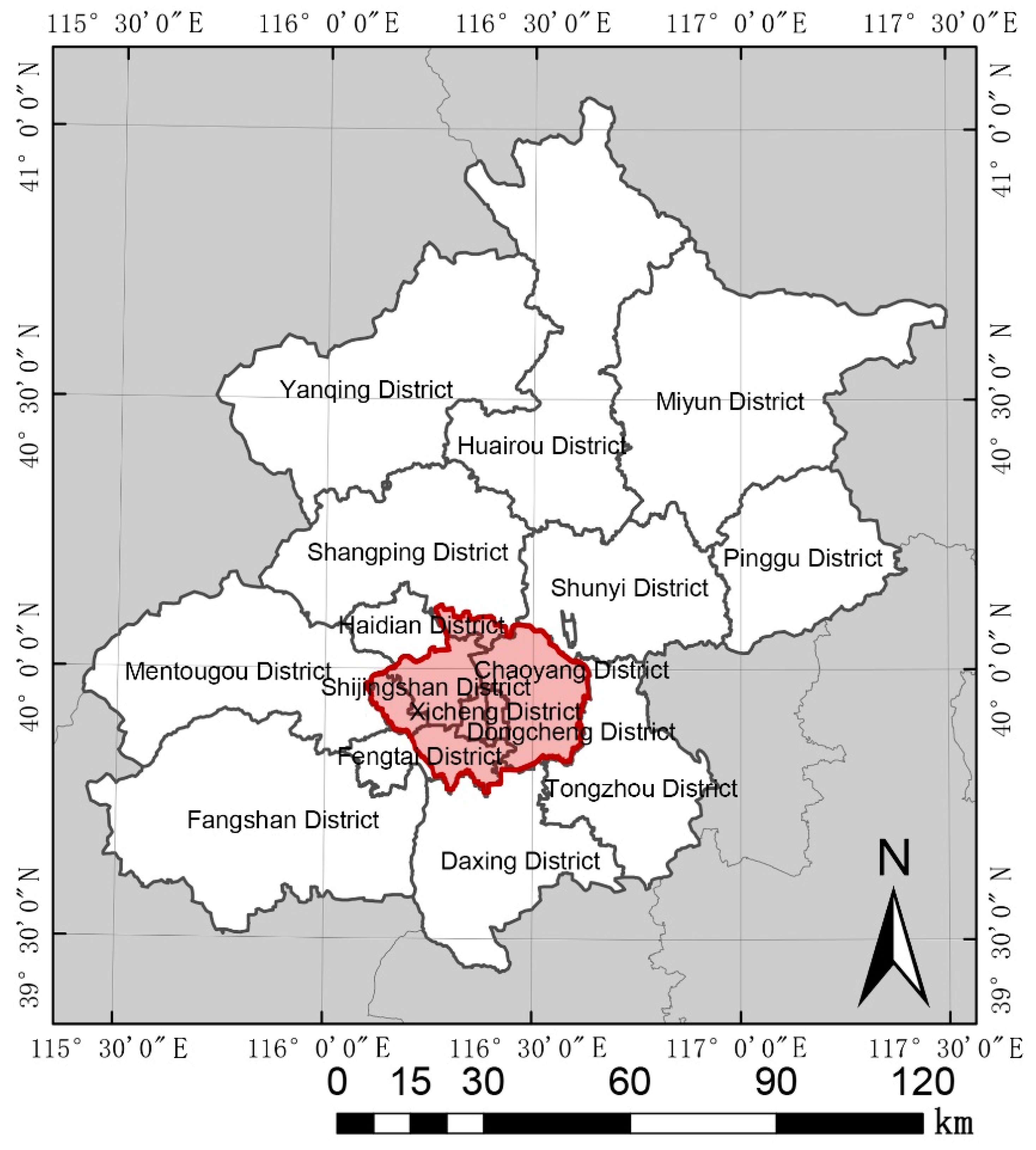
3.2. Construction of the SD Model for Conducting a Composite Simulation of Socioeconomic and Green Space Development
In this study, we predicted the green space area within Beijing’s central district, considered as a case study. The SD model incorporated macro socioeconomic factors, notably the demand for green space and the utilization of construction land [
51]. It simultaneously considered green space and land that could be supplied through future transfers, thereby establishing feedback relationships among various factors within the system to achieve a balance in the supply and demand of land between the area of green space and the socioeconomic system. Thus, the SD model mainly focused on the simulation and prediction of the amount of green space driven by macro socioeconomic factors to elicit macro policy inputs for the optimization of the area of green space in the study area. Micro factors were not considered in this study. The three main components of the SD model were a causal feedback chart used to describe the causal relationship between variables, a flow chart with symbols for expressing complex concepts in the model, and differential equations comprising the bulk of the model and connecting state variables and velocity. Most of the previous studies have applied the DYNAMO equation for operation. We obtained a portrayal of the overall system, including the economic and green space subsystems that changed continuously over time, by performing a simulation using the Vensim PLE software.
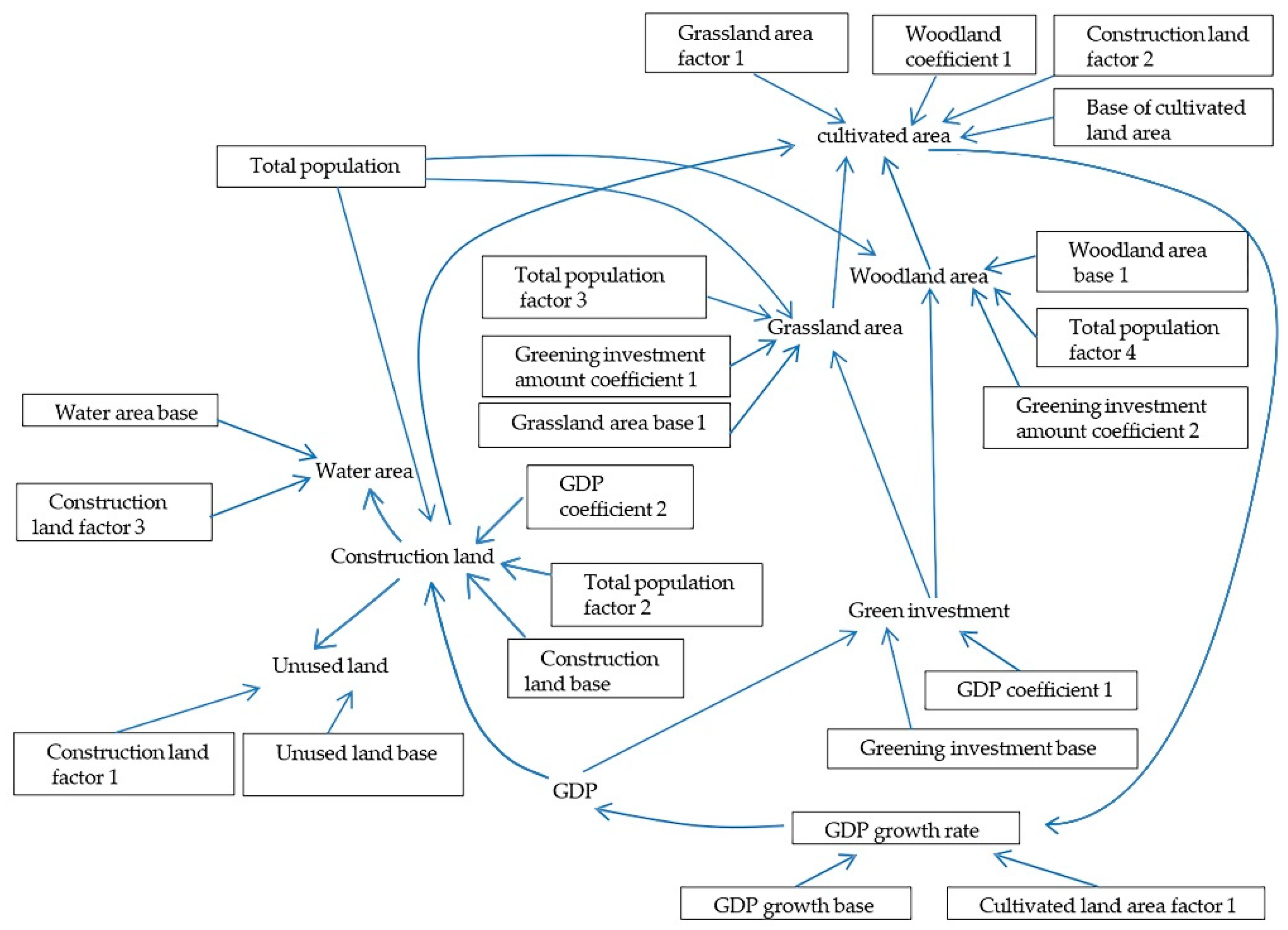
3.2.1. Construction of a Causal Feedback Chart for Simulating Green Space
The SD model constructed for this study mainly simulated the impacts of socioeconomic factors on the area of green space in the study area. Its results were used to analyze the interaction mechanism between the socioeconomic and green space subsystems. This composite system comprised several interactive feedback loops. The system’s overall functions were constituted through interactions among these loops [
52], ultimately leading to the formation of a closed green space composite system structure frame chart comprising socioeconomic and green space subsystems (
Figure 3). The model’s simulation covered a period extending from 1992 to 2050. The empirical and simulation verification stages extended from 1992 to 2016, and the forecast stage extended from 2016 to 2050. The base year was 2016, and the simulation step was one year.
The green space subsystem, which is a foundational component for ensuring the ecological security of Beijing’s central district, comprised three parts: (1) four types of green space, namely cultivated land, woodland, grassland, and wetland; (2) construction land related to green space; and (3) other types of land, such as unused land. The green space subsystem not only provides recreational resources for the socioeconomic subsystem but it also provides ecological services for the urban ecosystem. Therefore, this subsystem is a core component of the composite system. There are two types of factors that influence the area of green space. The first type comprises internal factors contributing to processes of growth and decline that lead to the expansion and reduction of the area of green space, mainly as a result of the conversion of cultivated land into woodland or grassland. The second type comprises external, mainly anthropogenic factors, notably the implementation of socioeconomic policies and urban construction. Certain green spaces are occupied for anthropogenic purposes relating to production and residence, leading to a reduction in the area of green space. However, increased construction of urban parks and afforestation activities results in significant expansion of woodland and grassland areas, thereby increasing the overall area of green space.
The socioeconomic subsystem could influence and regulate the binding force of green space through an increase in the population (the number of permanent residents), socioeconomic development (the GDP), and investments in construction and supply. At the same time, the development of the green space subsystem is restricted by the occupation of areas of green space. Thus, a complex dialectical relationship exists between the socioeconomic subsystem and the green space subsystem with two key effects. First, economic growth leads to increased investments in greening and improved living standards for people that strengthen the demand for and prioritization of green space. Consequently, areas of woodland and grassland may increase. Second, GDP growth leads to improvements in public infrastructure and social facilities in cities, thereby attracting an influx of people, resulting in a dramatic increase in the pressure exerted on the ecosystems of green spaces.
We used Vensim PLE software to establish a structure flow chart of the quantitative simulation of green spaces in Beijing’s central district performed with an SD model (
Figure 3) [
53]. The initial values of the main state variables in the model were derived from statistical data for the period 1992–2016. The values of some of the key constants and table functions were determined with reference to the development goals for Beijing’s socioeconomic development formulated in the 12th and 13th Five-Year Plans [
54,
55].
3.2.2. Construction of the Equation Used for Simulating the Area of Green Space
The data simulation and prediction of the SD model was mainly determined by the equation and system operation. Three types of parameters were applied: a constant parameter whose value did not change significantly over time, a table function that solved the nonlinear simulation in the equation, and an initial value derived from statistical data. The equations were mainly used to express the mathematical relationship between an indicator and its associated indicators in the model. We applied a combination of methods to determine the equation coefficients for a scientific green space composite system. First, we statistically determined the equation coefficients of a single dependent variable based on system data obtained for the period 1992–2016. The equation forms were expressed as linear regression, logarithmic, and exponential models. R2 was generally greater than 0.6, indicating that the equation form for the explanatory variable was reasonable. The formulas of these main indicators that meet the requirements of R2 are the preliminary formulas of the model. However, statistics can only guarantee the statistical relationship between a single independent variable and the dependent variable. Usually, an indicator is not only affected by a related factor, but the change of each indicator will affect another related indicator. Therefore, when adjusting other indicators, the simulated values of indicators that have met the requirements are also changing, and some of the predicted values of indicators no longer meet the requirements of inspection accuracy. At this time, we need to adjust the model. Therefore, it was necessary to adjust the parameters manually through system debugging to ensure that the results of the simulation of the main variables of the system met the accuracy requirements. When the accuracy of the main variables all meet the requirements, the parameters and coefficients in the model together form the final formula.
3.2.3. The Model Precision Test for Simulating the Area of Green Space
To ensure the reliability and scientificity of the green space composite system model, its validity had to be tested prior to the simulation. The error rate was calculated, and the validity of the model was judged through the performance of structure, unit, and Historical data tests [
56]. After conducting all of these tests, we found that the historical data as well as the simulation results met the error requirement within a 10% margin, indicating that the model was valid (
Table 1).
3.2.4. Scenario Design
We applied scenario analysis to optimize the area and spatial forms of green space. The results of this analysis reflected the uncertainty of urban development and considered existing and future urban development policies as a basis for predicting the future development of the city via models [
57]. We applied an SD model to simulate the green space composite system under scenarios entailing different speeds of economic development by changing the model’s parameters according to the historical data. We first selected indicators that were more sensitive to the system and had a greater impact on it and then established three scenarios (
Table 2) to enable the development of an optimization plan for Beijing’s green space.
Scenario 0 was a control scenario in which the current socioeconomic development trend was maintained and used for comparison purposes in the design scenario. Scenario 1 entailed moderate socioeconomic development and population control. The population of Beijing’s central district would rise to 9.29 million in the 19th step and an average GDP would be at growth rate of 6.1% in this scenario. In Scenario 2, the pace of economic growth would continue to decline, and the population would be further reduced. The population of Beijing’s central district would reduce to 8.59 million during the 19th step and the average GDP growth rate would reduce to 4.9%.
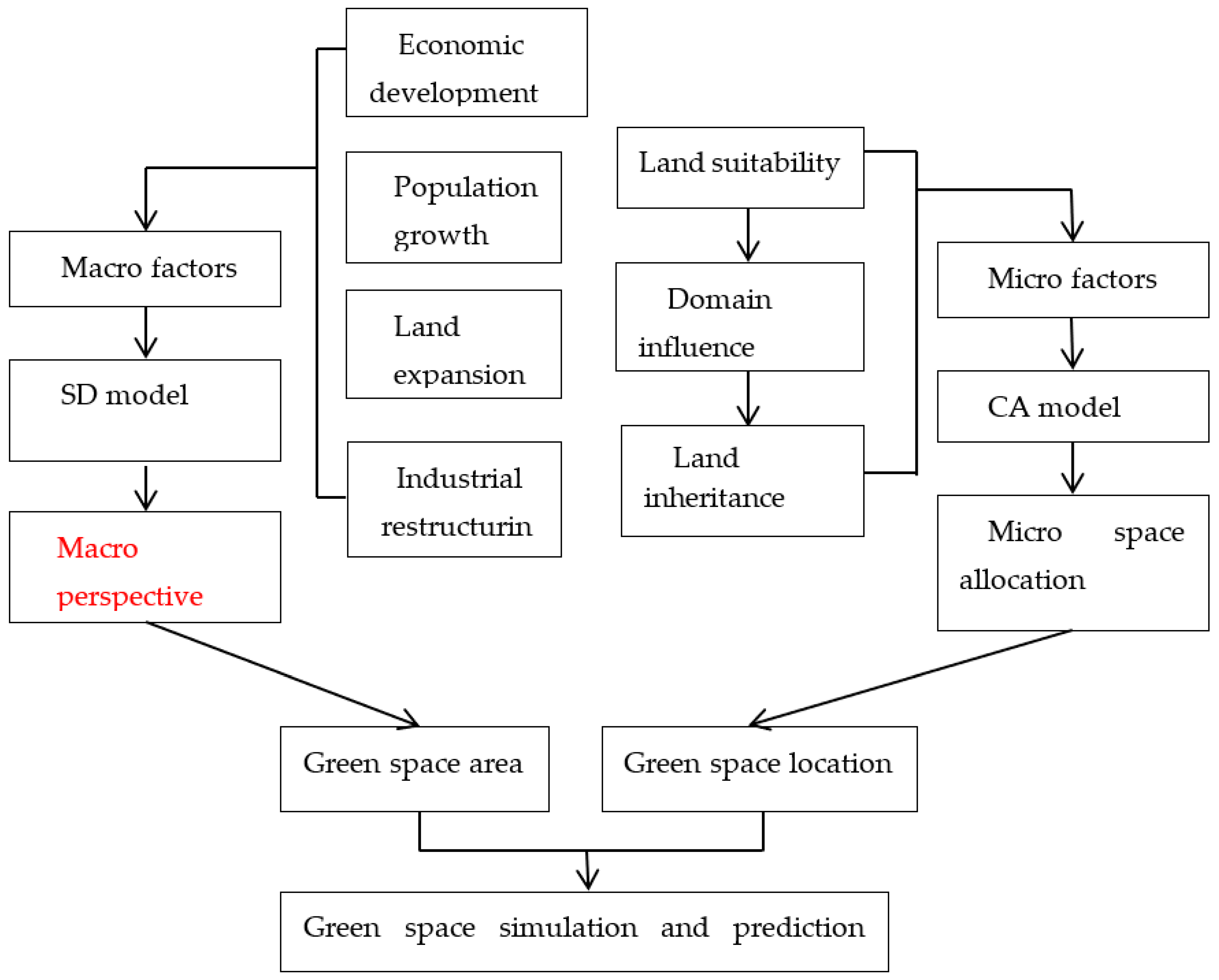
3.3. The CA Model Used to Simulate Green Space in Beijing’s Central District
Because natural conditions could limit and affect the evolution of green space, we first deployed the powerful space simulation capabilities of the CA model, referring to existing research and the actual development of green space in Beijing’s central district. Our aim was to determine the possibility of converting land into green space, considering conversion suitability, influence of neighborhoods, and green space inheritance. The CA model has been widely used to simulate these variables, with each specific indicator obtained on the basis of a transformation rule and a thorough review of studies and data on land-use status in Beijing’s central district [
58,
59,
60]. Considering the total forecasted results of the SD model in the scenario simulation, we simulated and predicted the spatial distribution of green space in Beijing’s central district under different economic development trends (
Figure 4).
- (1)
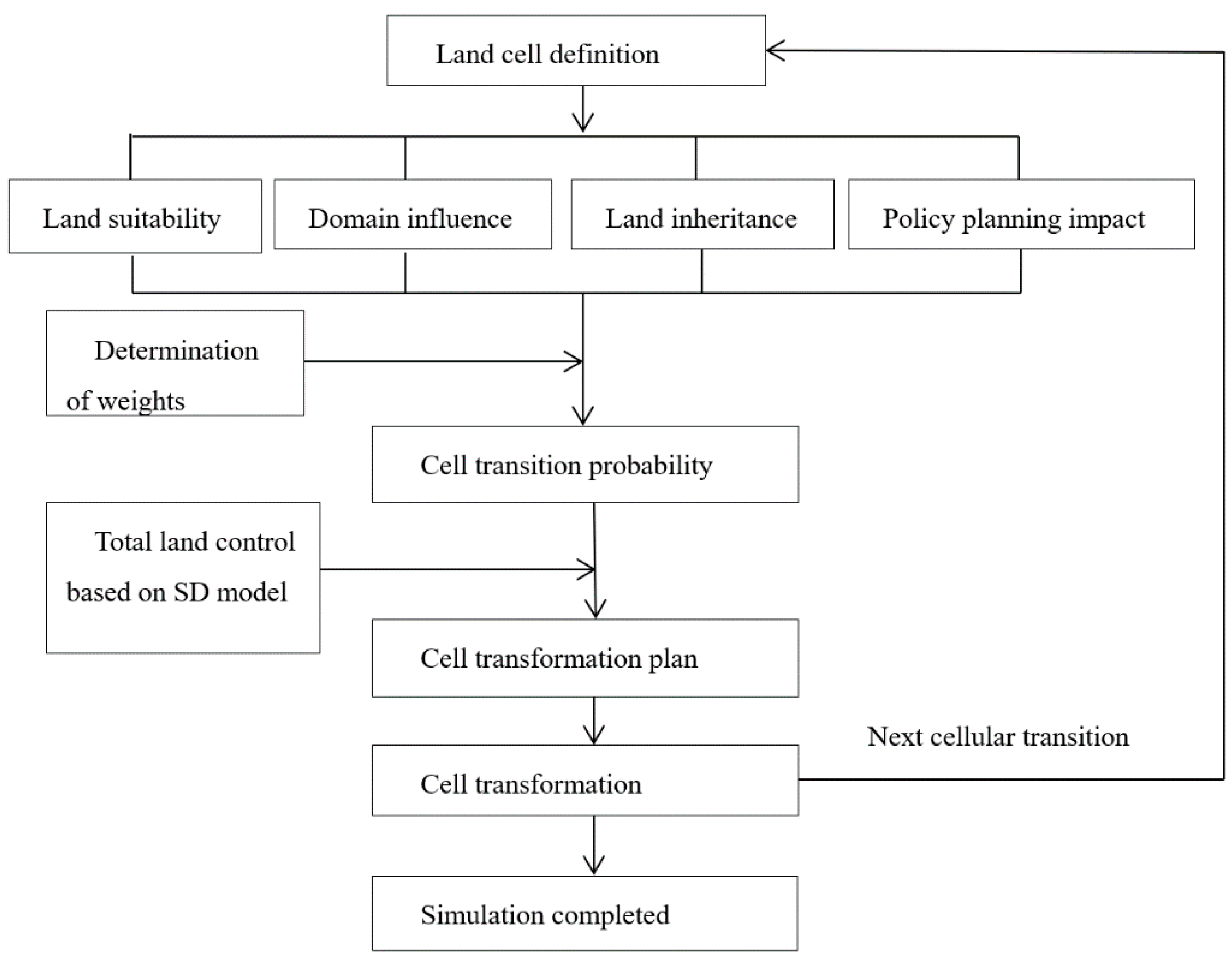
Cell Definition
The process of defining land cells entailed rasterizing the remote sensing data in ArcGIS, which had an accuracy of 30 m, with each cell unit having an area of 30 m × 30 m.
- (2)
Calculation of the Probability of Cell Conversion
The probability of land cell conversion was determined by factors influencing the suitability of land conversion, the influence of neighborhoods, and land inheritance. Existing studies have generally incorporated planning-related factors into calculations of probability. Those factors comprise different variables with varying rates of contribution to land conversion. Therefore, it was necessary to determine the weight of each variable which could then be inserted through a reasonable mathematical formula to calculate the probability of each cell being converted to another cell type.
- (3)
Determination of Conversion Rules
The conversion of land cells depended on the conversion rules. Generally, cells with a higher probability of land conversion had a higher probability of conversion. The number of cell conversions was determined by the total amount simulated in the SD model. Given this constraint on the quantity of cells, we selected the cell to be converted according to the probability of its conversion. Upon completion of each simulation, we repeated the calculation for the probability of cell conversion to guide the next cell conversion.
- (4)
Validity Check
In the CA model, the weight setting for factors relating to the suitability of land conversion, neighborhood influence, land inheritance, and policy planning determined the probability of land cell conversion in the CA model and affected the results of the spatial simulation of land. Therefore, it was necessary to revise the simulated spatial data on the basis of historical land interpretation data and to use the Kappa coefficient as the accuracy standard for verifying the simulation results [
61].
3.3.1. Simulation of the Probability of Land Conversion into Green Space
The CA model was used to determine the probability of land conversion into green space based on the suitability of the conversion, neighborhood influence, land inheritance, and the impacts of policy and planning (
Table 3). In this study, we defined the probability that the land cell at position (
x, y) would be converted into
K-type land during period
t as
tPK,x,y. The suitability of
K-type land for conversion was defined as
tSK,x,y, the impact of the neighborhood on the conversion of a land cell into
K-type land was defined
as tNK,x,y, the inheritance of the land itself was defined as
tIK,x,y, and the impact of planning factors on the conversion was defined as
v. Thus, the probability of the land cell being transformed into
K-type land was expressed as:
The specific calculation was as follows:
The suitability of land conversion was assessed in terms of the distances between the land and the road and the city center, the suitability of the land conversion in relation to the slope, and the land grade assigned to agricultural land in terms of its protection status. The following formula was used for the calculation:
where
denotes the standardized value of the land suitability factor and
denotes the weight of the suitability factor.
Given differences in the distances between different types of land and the road and the city center, we applied the following formula to determine the suitability of
K-type land from location (
x, y) to the nearest road and the city center,
r, at a certain time point:
where
Dr denotes the distance between the location of a land cell (
x, y) and the nearest trafficable road. Because each land cell had different requirements relating to road accessibility, the correction coefficient for the accessibility of a trafficable road from a construction land unit was set to 100, and correlations for wetland and water bodies and cultivated land units were set at 50 and 10, respectively.
The suitability of different land types in relation to their slope also differed. In general, the suitability of land for cultivation had a value of 0 when the slope exceeded 25 degrees, and a value of 1 when the slope was below 25 degrees. Slope had no effect on woodland, wetland and water bodies, unused land, and grassland. The impact of slope on construction land was standardized using the following formula:
The Land and Environmental Protection Agency of the Beijing Municipal Planning Commission has explicitly advocated the protection of agricultural land in Beijing. Therefore, the probability of land conversion was determined on the basis of land grades assigned by the Land and Environmental Protection Department according to the suitability of agricultural land for cultivation.
The influence of neighborhoods (tNk,x,y) was determined based on the surrounding land types. We considered 5 × 5 neighborhood units and standardized the tNk,x,y values according to the number of K-type land units in a neighborhood.
Green space, construction land, and unused land all had varying degrees of stability relating to their inheritance status (tIk,x,y). In the CA model, the stability of the land was set as a constant value to express the land unit’s inherited status. A lower value corresponded to lower inheritance, and a greater possibility of its transfer. Fifteen experts from government agencies and universities offering urban planning and environmental science as majors were surveyed. We set the inheritance values of cultivated land, woodland, grassland, wetland and water bodies, construction land, and unused land at 0.60, 0.75, 0.40, 0.75, 1.00, and 0.00, respectively, according to the scores assigned by the experts.
The probability of land conversion into constructed land and woodland in the southeastern part of the central district increased by 0.3 and 0.1, respectively. This calculation was based on a consideration of linkages existing between land-use planning and the planning and construction of key green spaces relating to the construction of the new city of Tongzhou in Beijing.
3.3.2. Conversion Rules for Green Space Simulation
We performed space allocation simulations of Beijing’s green space, construction land, and unused land based on the various land area requirements determined using the SD model.
Rule 1: The CA model was used to simulate spatial conversions between green space and construction and unused land. The following conversions were considered based on the current status of land use in the central district area and a literature review.
Cultivated land could be either protected—and was therefore not transferable—or transferred. Cultivated land that was transferable could be converted into construction land (for urban expansion and construction), woodland (plain afforestation or conversion of cropland into forests and parks), grassland (park and golf course construction), and wetland and water bodies (park construction and the restoration of water systems).
Woodland could be protected—and therefore not transferable—or transferred. Woodland that was not protected could be converted into construction land (for urban expansion and construction), grassland (for park and golf course construction), or wetland and water bodies (for park construction and the restoration of water systems).
Grassland could be converted into grassland, construction land (for urban expansion and construction), woodland (for park construction), or wetland and water bodies (for park construction and the restoration of water systems).
Wetland and water bodies could be converted into wetland and water bodies, construction land (for urban expansion and construction), or woodland (park construction).
Construction land could be converted into construction land, woodland (park construction), grassland (park and golf course construction), or wetland and water bodies (park construction and the restoration of water bodies).
Unused land could be converted into unused land, construction land, woodland (park construction) and grassland (park and golf course construction).
Rule 2: The total amount of land determined in the SD model simulation would be allocated in the following order: construction land, cultivated land, woodland, grassland, wetland and water bodies, and unused land. After allocating the total amount of land of the first type, allocation of the second type of land would be carried out. Moreover, after completing the conversion of one type of land, it would not be converted again during the simulation period.
Rule 3: A land cell at (x, y) location was defined as tPK,x,y relating to land selection according to the probability of its conversion into K-type land in period t. Cell units with a higher probability of being converted into K-type land than other land types in Beijing’s central district would be selected first. These cell units would be selected in descending order of the probability of their conversion until the total demand for K-type land was satisfied.
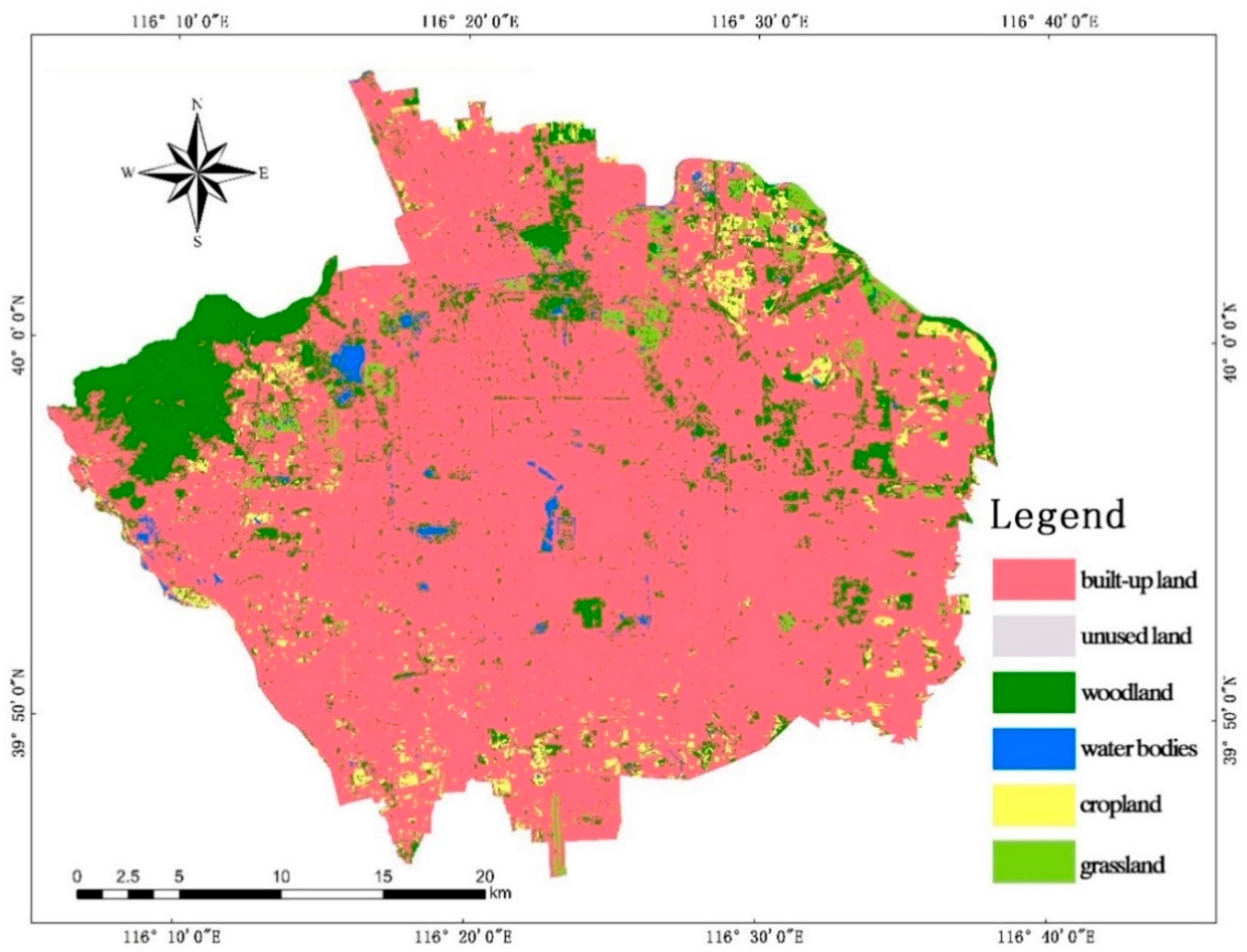
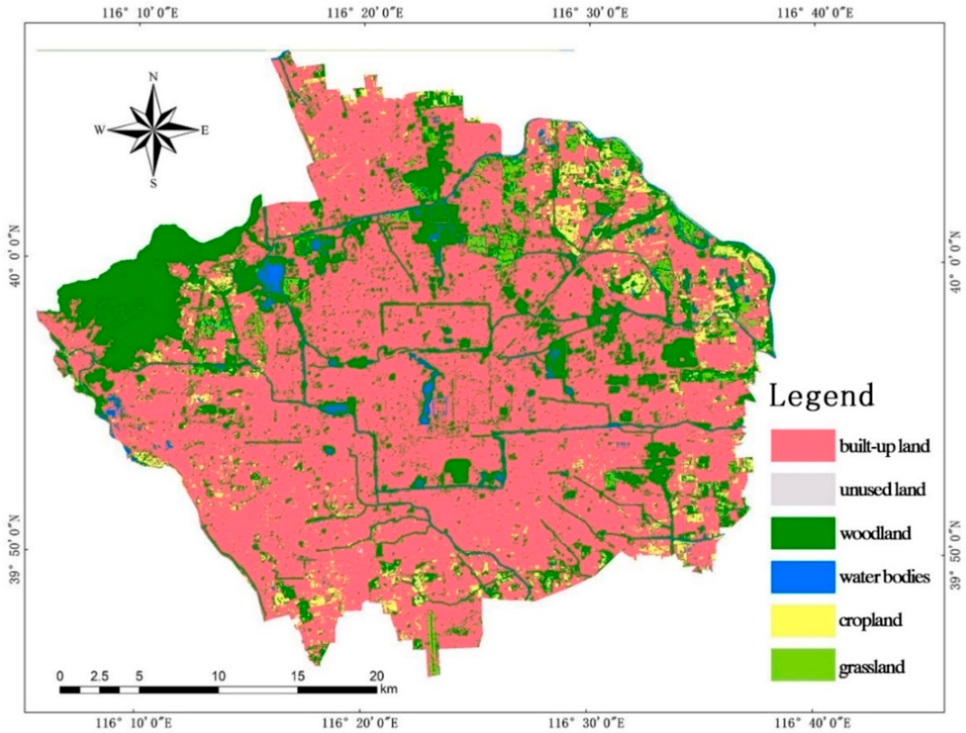
3.3.3. Verification and Revision of Green Space Simulations
The weight setting of the influence of neighborhood size and inheritance based on different factors would affect calculations of the probability of converting different green spaces and hence the simulation results. Therefore, it was essential to revise the spatial model using relevant data. We conducted simulations based on land interpretation data for Beijing’s central district in 1992 and 2000 and revised the simulated data for 2008 and 2016. The Kappa coefficients for the simulation results in 2008 and 2016 were 0.7813 and 0.8076, respectively, which met accuracy requirements.


