Abstract
While deforestation is a major environmental issue in the tropics, with thousands of hectares converted to agricultural land every year, in Europe the opposite trend is observed, with land abandonment in mountainous and semi-mountainous areas allowing the afforestation of former agricultural and pastoral land. This trend allows semi-natural ecosystems to recover after a prolonged period of exploitation and often over-exploitation, but it may also lead to significant loss of landscape heterogeneity with potentially detrimental effects on biodiversity. The current study aims to monitor changes in the vegetation coverage across a period of 35 years (between 1984 and 2019) in the Rhodopi Mountains range National Park in northern Greece. A time series of LANDSAT TM (16 images), LANDSAT ETM + (1 image) and LANDSAT 8 OLI/TIRS (4 images) were employed. One data transformation method was applied (TCT), and five vegetation indices (NDVI, NDWI, SAVI, EVI2 and BSI) were calculated to capture the land cover transition during the study period. The obtained results and all used indices suggest that over the study period there was a continuous trend of vegetation cover increasing, with open areas decreasing. The observed trend was further confirmed using Object Oriented Image Analysis on two pairs of images sensed in 1984 and 2019, respectively. The results suggest that almost 22.000 ha of open habitats have been lost to broadleaved and conifer woodlands, while the former also appear to be advancing into conifer-covered areas. This trend has led to significant loss of landscape heterogeneity and to a broadleaf-dominated landscape. The results are discussed in relation to their driving forces, the potential implications on biodiversity and the risk of wildfires in the near future.
1. Introduction
The outbreak of the Industrial Revolution in Europe in the 19th century signified the beginning of two very important changes in Western societies: the urbanization of the population and the intensification of production, whether it concerned the newly entered industrial production or agricultural and pastoral production [1]. The combination of these two factors gradually intensified in the early 20th century. The abandonment of mountainous and semi-mountainous areas and the establishment of these populations in cities and urban areas allowed the intensification of agriculture and stock breeding and production increase [2]. This phenomenon was further intensified during the second half of the 20th century and, in the decade 1990–2000, involved the abandonment of 20 Mha in 20 European countries, marking significant changes in land cover and use [3]. This Land Use/Land Cover (LULC) change has increased the extent of forests in Europe by 9% in the last 30 years. Approximately 227 Mha, more than the third of Europe’s land, is now forested [4]. Although the abandonment of marginal agricultural land in the Mediterranean region, followed by natural vegetation recovery, has been maximized in the 1960s, 1970s and early 1980s [5], it is still a major trend that requires attention and research [6,7,8].
Ιn Greece, the population trend followed the pattern of decreasing rural populations and increasing urban ones. The mass exodus of the mountain population began in the 1940s and was largely due to the conflicts of the civil war and the persecution that followed the years of national resistance to the German occupation. The large scale abandonment of the mountainous and semi-mountainous areas was maximized during the period of mass migration from small rural villages to big cities and foreign countries in the 1950s, 1960s and 1970s [9,10]. It is worth mentioning that during the period 1987–1993 the number of agricultural holdings in the mountainous areas decreased by 15.7% and the agricultural land by 12.8%. At the same time the corresponding numbers for the whole country were 14.1% and 6.9%, which indicates that the decrease in the number of holdings is not due to a possible merging and increase in their size, but to the abandonment of agricultural land [9,10].
Livestock farming, which was mainly nomadic, underwent similar pressures. In 1923, 13,700 families were engaged in nomadic grazing, with a sheep and goat stock of about 2.5 million animals [10]. By 1960 the number of livestock fell to 2 million animals with a corresponding increase in stable livestock, while by 1984 the mobile livestock had decreased by 27.5%, and the stable one increased by 15.6% [10]. All these trends, and in combination with the aging of the remaining population, resulted in the abandonment of activities in mountainous and semi-mountainous areas with forests growing at the expense of meadows and agricultural land. Through secondary ecological succession, meadows were gradually transformed into shrubby vegetation and, finally, into forests [11]. This resulted in a reduction in the fragmentation of forests in the agro-pastoral landscapes, while pastures reduced in size and the distance between them increased [12].
Therefore, land abandonment is considered one of the main drivers of LULC changes, with significant environmental and socio-economic implications that can be positive or negative, depending on local factors and conservation objectives [13]. Recovery of forests can reduce soil erosion, increase biodiversity and create carbon reservoirs [14]. However, it can also lead to the reduction of many semi-natural, open habitats previously maintained by traditional land management, having a significant impact on the landscape, biodiversity, ecosystem, dynamics and sustainability of mountainous landscapes [15].
Keenleyside and Tucker [16] reported that, in some cases, the re-colonization of plants and the disappearance of open spaces endanger semi-natural habitats by causing reduced biodiversity. However, in other cases, abandonment can be beneficial as it helps to restore natural habitats, especially in landscapes that are highly fragmented by human activity [17]. Consequently, systematic monitoring and detailed recording of LULC change and trends are becoming increasingly necessary, both for economic and environmental reasons, as they can be key indicators of environmental/ecological change at different spatial and temporal scales [18]. Monitoring land use changes with time and cost-efficient methods is essential for reducing biodiversity loss and for implementing Streamlining European Biodiversity Indicators 2020 (SEBI 2020) [19].
Recent advances in remote sensing data availability, quality and methods offer a great tool for the long-term monitoring of LULC trends [20]. Remote sensing data covering a wide part of the electromagnetic spectrum, including near and short-wave infrared channels, allow the calculation of a large number of vegetation indices. The latter are designed to enhance the vegetation signal to allow reliable spatial and temporal comparisons of terrestrial photosynthetic activity and canopy cover [21].
In recent decades, LULC monitoring using remote sensing data has significantly improved spatial and thematic accuracy of the resultant products, mainly because of the development of new technologies and applications along with appropriate algorithms for data analysis. Crucial in this area is NASA’s Landsat program, which, since 1972, has provided the repetitive acquisition of multi-spectral, high-resolution Earth Observation data on a global basis leading to the largest database of the Earth’s surface [22,23,24,25,26,27]. The release of the program data for public use free of charge, through the Earth Resources Observation and Science (EROS) center, has made it possible to easily access an unprecedented volume of data, opening new horizons in the detection of changes in the earth’s surface [28].
The aim of this study is to investigate diachronic vegetation changes (since the early 1980s, when agricultural abandonment reached its peak) in the Rhodopi Mountain Range National Park using multitemporal landsat data. The specific objectives are (a) to investigate the degree of vegetation densening and loss of open habitats using a number of vegetation indices that are often employed for long term monitoring, (b) to quantify the observed changes and (c) to discuss the observed changes in relation to the implications on biodiversity and fire risk.
2. Materials and Methods
2.1. Study Area
The study area is the Rhodopi Mountain Range National Park (henceforth RMRNP) in northern Greece (Figure 1), which occupies approximately 175,000 ha with an altitudinal range of 50–2022 m a.s.l. It is located at the central-west massif of the area of the Rhodopi mountain range, constituting a natural border between Greece and Bulgaria. The Rhodopi Mountain Range is shared between the two countries, occupying a total area of 1,473,500 ha. Approximately 82% of the total area of Rhodopi is located in Bulgaria and 18% is in Greece.
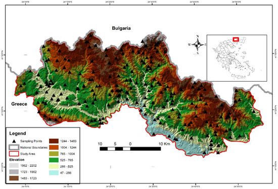
Figure 1.
Location of the study area and landscape and oreographic characteristics.
The ecological significance of the ecosystems in RMRNP has resulted in the designation of larger or smaller areas into various national and international protection regimes. In particular, seven areas of the RMRNP have been included in the Natura 2000 network of protected areas (two of them as Special Protected Areas and five as Special Areas of Conservation), two areas have been declared as Preserved Natural Monuments, seven areas as Wildlife Reserves, and three areas have been characterized by the European Council as Biogenetic Stocks.
The climatic conditions represent a transitional zone between sub-Mediterranean and central European with a wet continental character. The mean annual temperature is 10.3 °C, and the average annual precipitation is 875.3 mm [29]. Inside RMRNP a rich variety of ecosystems of the Balkan Peninsula are to be found. Almost 60% of European species can be found here, and this is the main reason that makes RMRNP one of the most important regions for European nature conservation. Inside the area, 26 different habitat types exist and all the vegetation zones of Europe, from the euro-Mediterranean zone of the evergreen broadleaves to the zone of cold resistant conifers and sub-alpine meadows. Its main land cover types are coniferous stands of black pine (Pinus nigra J.F. Arnold), Scots pine (P. sylvestris L.), Norway spruce (Picea abies L.), broadleaved stands of beech (Fagus sylvatica L.), silver birch (Betula pendula Roth), oaks (Quercus sp.), evergreen broadleaves, open areas, maintained by anthropogenic activities and especially grazing, as well as a small proportion of agricultural areas. The RMRNP is also rich in wildlife biodiversity, accommodating species such as Brown Bear (Ursus arctos), grey wolf (Canis lupus), red deer (Cervus elaphus), roe deer (Capreolus capreolus), Chamois (Rupicapra rupicapra ssp. balcanica), wild boar (Sus scrofa), Capercaillie (Tetrao urogallus), Grouse (Bonasa bonasia), golden eagle (Aquila chrysaetos) and others [30].
2.2. Remote Sensing Data
Overall, 120 Landsat images (Path:183, Row:031) were downloaded from the EROS center, while 21 of them were selected to build a time-series dataset covering a period of 35 years (Table 1). The rest were excluded from the analysis, either due to extensive cloud cover/shading or line stripping of Landsat 7. The sensing period of the selected images was between the 1st of August and 16th of September. This particular time window was selected because it corresponds to the driest period in the study area, when annual herbaceous vegetation had died out. Since the study focuses on the densening of woody vegetation the absence of live herbaceous vegetation is expected to aid the analysis, which is based on vegetation indices. All images were obtained pre-processed at level 2A (geometrically and atmospherically corrected to BoA reflectance) by the EROS center. These images provided by the Landsat program, apart from being geometrically and atmospherically corrected, have a radiometric resolution of 16-bit, which makes it easier to compare between the three sensors. However, L2SP Tier2 products such as the 1984 and 1993 images required geometric correction to spatially match the rest of the images. Thus, both images were geometrically corrected by registration to the 1987 image using 31 ground control points (GCP).

Table 1.
Satellite Images used in the study.
The Landsat series provides earth observation data since 1972 at varying spectral and spatial resolutions (Table 2). Since 1982, when Landsat 4 was launched, the spatial resolution has remained stable at 30m for the multispectral products. Due to the long time span of Landsat data availability, they are quite extensively used to build time series datasets for long term monitoring of vegetation dynamics [22,23,24,25,26,27]. The Thermal and Coastal/Aerosol bands were excluded from the analysis as well as the panchromatic image.
Table 2.
Spectral and Spatial characteristics of the Landsat images used in this study.
2.3. Remote Sensing Data Analysis
Two techniques were employed to monitor woody vegetation cover changes in RMRNP: the Tasseled Cap Transformation (TCT) [31] and the implementation of Vegetation Indices (VI’s). The TCT algorithm represents empirical equalization of spectral channels and linear transformation of bands to three indices: brightness, greenness and wetness. Brightness is usually associated with bare or sparsely vegetated lands, greenness with green vegetation, and wetness is usually associated with moisture, water and other moist features [32].
Recording and monitoring vegetation changes using Vegetation Indices is a relatively fast process that allows a good understanding of changes in space and time. In the current study, five VI’s were used, which were selected based on their capability to capture vegetation variation in an image, as it is documented in the literature. The specific properties of each of the employed vegetation indices are provided in the following paragraphs. The five indices were the Normalized Difference Vegetation Index (NDVI), Soil Adjusted Vegetation Index (SAVI), Enhanced Vegetation Index 2 (EVI2), Normalized Difference Water Index (NDWI) and Bare Soil Index (BSI; Table 3).
Table 3.
Vegetation Indices and Spectral Ratios employed in the study.
NDVI is one of the vegetation indices that combines the two opposite properties of canopy. It is known that the spectral profiles from green vegetation represent two specific areas where the highest discrepancy occurs (red to nir region) [33]. Because of this property, NDVI is considered an appropriate vegetation index to study vegetation patterns across temporal or spatial scales, and it has been extensively used in such studies [26,38,39,40,41]. SAVI is based on the original NDVI formula and is a transformation technique that minimizes the effect of soil brightness. It has been found to give better results than NDVI in cases of high variation in soil color and moisture [34]. EVI was developed to optimize the vegetation signal with improved sensitivity in high biomass regions and improved vegetation monitoring through a decoupling of the canopy background signal and a reduction in atmosphere influences [35]. NDWI [36] is an index derived from the Near-Infrared (NIR) and Short Wave Infrared (SWIR) channels. The SWIR reflects variation in both the vegetation water content and the spongy mesophyll structure in vegetation canopies, while the NIR reflectance is affected by leaf internal structure and leaf dry matter content but not by water content. The combination of the NIR with the SWIR removes variations induced by leaf internal structure and leaf dry matter content, improving the accuracy in retrieving the vegetation water content [42]. Bare Soil Index (BSI) is a numerical indicator that combines blue, red, near infrared and short wave infrared spectral bands to capture soil variations. These spectral bands are used in a normalized manner. The short wave infrared and the red spectral bands are used to quantify the soil mineral composition, while the blue and the near infrared spectral bands are used to enhance the presence of vegetation. The original BSI [43] used SWIR1 reflectance, but recent research by Diek et al. [37] suggests that the SWIR2 band may be more appropriate for calculating BSI. For this reason, the SWIR2 band was used in this study to calculate BSI index.
All the above indices and transformations were calculated for the entire set of Landsat images. In order to reduce the effect of interannual variation caused by subtle differences in the vegetation phenological characteristics and the sun’s geometry, all indices were stretched to a range of −1 to 1 using Equation (1). The equation was applied to all Vegetation Indices calculated for the study area and for all time slots (105 times in total).
where: VIrescaled = The stretched value of the respective Vegetation Index (NDVI, SAVI, EVI2, NDWI, BSI); VI = The value of the Vegetation Index as calculated using the respective formula; VImin = The lowest value of the Vegetation Index across the image; VImax = The highest value of the Vegetation Index across the image.
One thousand points were randomly located across the entire study area, using the Sampling Design Tool, available as a plugin in ArcMap (v.10.8, Esri Inc., Redlands, CA, USA) and these formed the basis for the determination of vegetation dynamics across the time span of the study. The vegetation index values of the pixel corresponding to each particular point are then assigned as attributes to the point. Linear regression was employed to test for significant relationships between the tested vegetation indices and time. Furthermore, Mann Kendall test was used to test for significant trends between time and vegetation indices [44].
Once the pattern of vegetation dynamics had been established, an Object Oriented Image Analysis (OBIA) was employed and applied to the images of the first year (1984) and the last year (2019) of the study in order to quantify the vegetation changes. For each time slot an additional Landsat image, acquired during the winter season, was employed. Four classes were identified in 2019 (open areas, broadleaved forests, coniferous forests and water bodies). In 1984 three classes were identified (water bodies was excluded) because the water body present in the area in 2019 resulted from the construction of two dams during the study period.
The OBIA, which was conducted using the software eCognition v.10.2 [45], was found to be an effective approach in capturing the landcover variation of the Mediterranean mountain regions [46,47,48]. The first step of OBIA is the generation of objects consisting of spectrally similar neighboring pixels using an appropriate scale parameter. The objects are then classified using training samples in a preset classifier or crisp and fuzzy rules. The classification is performed based on the image spectral information, or ancillary data, which for this study were three layers representing elevation, eastness and northness, respectively, all generated using the ASTER Global Digital Elevation Model (GDEM). The scale parameter was set at 100, with testing scale parameters between 10 and 150 (at intervals of 10) and with visual assessment of the segmentation result for over and under segmentation. The color criterion was set at 0.7 and the shape at 0.5. Various classifiers, including Classification Trees (CART), Support Vector Machines (SVM) and Random Forests (RF), all embedded in eCognition, were tested for their effectiveness in identifying the selected classes. The evaluation of each classifier’s performance was assessed by their efficiency in reproducing the training set [46]. Among the ones tested, Support Vector Machines (SVM) was found to have the best performance.
For training the classifier and testing the result for the year 2019, we employed 200 sampling points, located randomly and sampled in May–August 2019. The vegetation composition in these 200 points was estimated in circular plots with a radius of 17.9m, which resulted in a plot of approximately 0.01ha. The delimitation of each plot was made using the TruPulse 200R Laser range finder. The sampling protocol included a visual estimation of canopy cover and the relative abundance of species using the 9 scale Braun Blanquet approach. From the 200 collected plots, 150 were used for training and 50 for testing the results. The same training and test data were used for the 1984 classification after removing the plots that had changed within this period. The assessment of the degree of change was based on a change index calculated using selective Principal Components Analysis (PCA), which was applied to the two summer Landsat images of 1984 and 2019 [49,50]. According to this approach, from a pair of images, a set of comparable layers are selected, which in this case were the six spectral bands of the Landsat images. A selective PCA analysis is performed for each pair of comparable layers to obtain two principle components in the two dimensional feature space, where the first (PC1) expresses the information common to both pictures and the second (PC2) expresses changes between the two images or noise. The change intensity increases towards the margins of PC2. To convert the PC2 values into change index values and to separate between actual change (increasing towards the margins of PC2) and noise (central part of PC2) the absolute difference values of a bidirectional normalized sum function are calculated [51]. This fuzzy membership function assigns values of around 0 to the pixels that occupy the central part of PC2 and increases values towards 1 as the pixel’s location approaches the margins of PC2. The closer the values are to 1 the higher the possibility of change [51]. The approach has been successfully employed in the Mediterranean environment for monitoring post fire vegetation recovery [52]. In this study, a threshold of 0.7 was used, above which a pixel is considered to have changed. This resulted in 112 points for training and 36 for testing the classification result of 1984.
Based on the two mapping products of the two time slots, a transition matrix was constructed in order to quantify the change and identify its pattern. Furthermore, two landscape diversity indices were calculated, the Shannon’s Diversity and Evenness indices, in order to see if the observed changes had resulted in increased homogeneity or heterogeneity. The calculation was performed using the Patch Analyst extension for ArcMap [53]. Finally, a multitemporal spectral profile of the main transitions was constructed based on the NDVI values. The flowchart adopted for this study is shown in Figure 2.
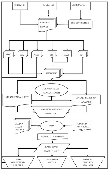
Figure 2.
Flowchart of the study.
3. Results
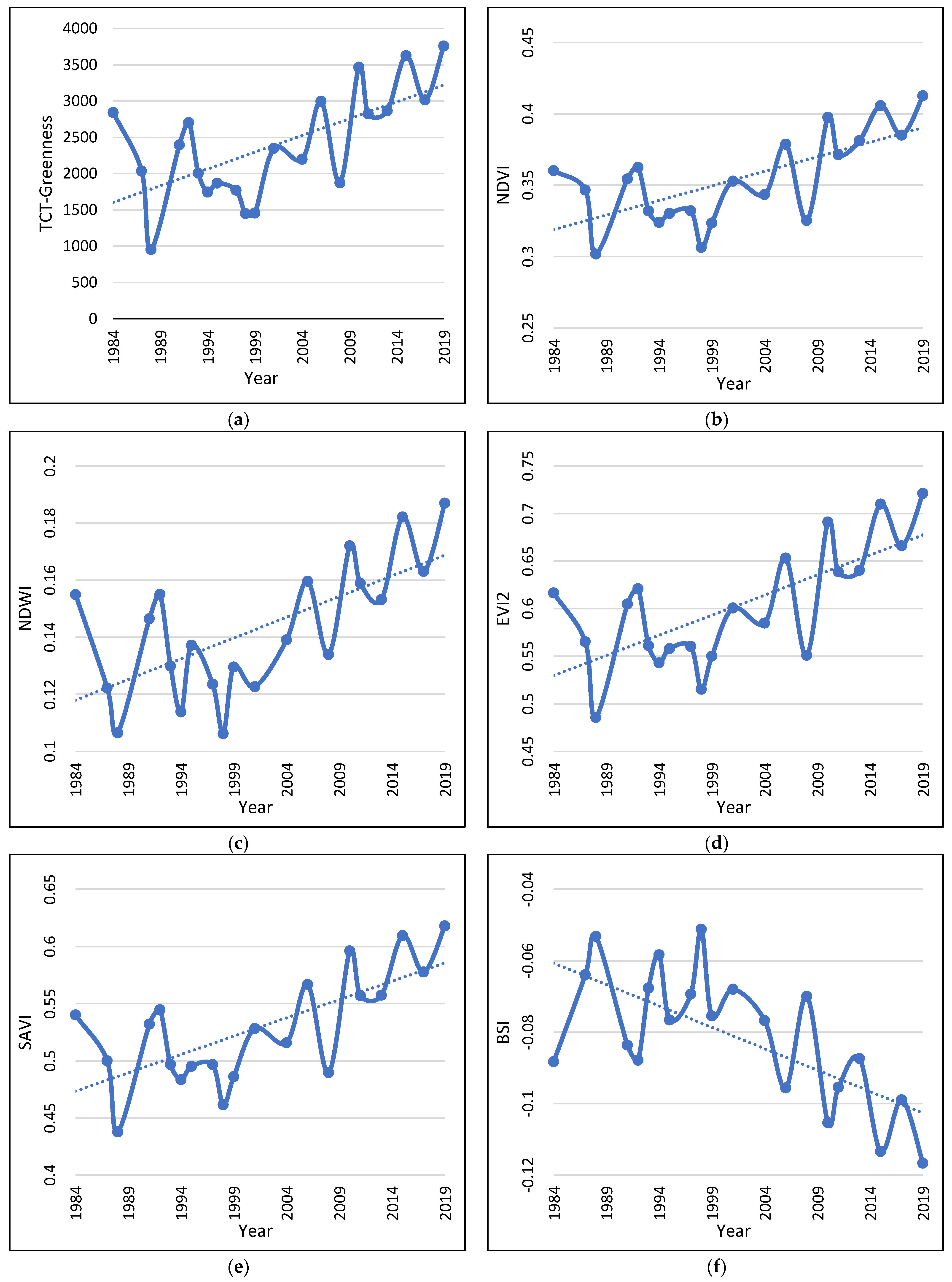
The linear regression analysis revealed a statistically significant relationship only between Greeness and time and the Mann–Kendall test confirmed a statistically significant positive trend with time (Table 4; Figure 3a). The rest had neither statistically significant relation with time nor any significant positive or negative trend.
Table 4.
Results of the linear regression between time and the TCT indices and Mann–Kendall test.
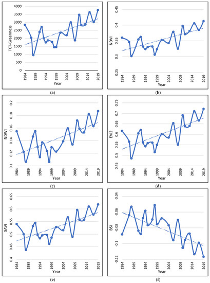
Figure 3.
Vegetation Indices dynamics and trend during the study period (a–f). The graphs are built based on the 1000 randomly located points, corresponding to 1000 pixels.
The tested vegetation indices, on the other hand, all show statistically significant relationships with time and statistically significant positive or negative trends during the study period (Table 5; Figure 3b–f). The results clearly indicate that, during the study period, the vegetation cover of the study area increased significantly.
Table 5.
Results of the linear regression between time and vegetation indices and Mann–Kendall test.
All indices that were sensitive to the existence of vegetation exhibited a positive trend during the study period (Figure 3b–e), while the BSI, which is sensitive to bare ground exhibited a negative trend (Figure 3f). BSI is an index that constitutes a combination between a vegetation index and a bare soil index and tends to obtain higher values in the least vegetated areas [37]. Both these results demonstrate that vegetation increased its density significantly during the study period as a result of several factors that will be discussed later. This result was further confirmed by the OBIA classification in the two time slots.
The OBIA classification for the two time slots (1984, 2019; Figure 4) revealed important landscape differentiations during the study period and confirmed the previously reported result. The classification accuracy assessment of the 2019 classification shows an overall classification accuracy of 92% and kappa statistics of 0.78, and of the 1984 an overall accuracy of 91.6% and kappa statistics of 0.85.
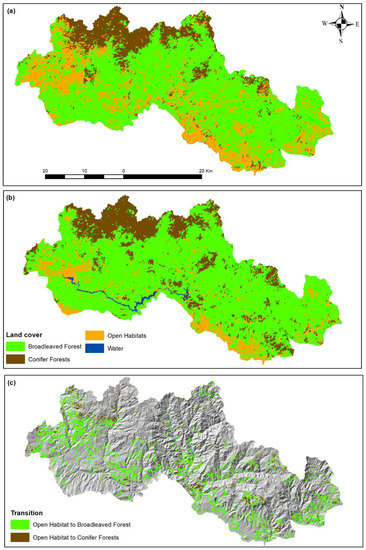
Figure 4.
Landcover maps of the years 1984 (a) and 2019 (b) and transition map from open habitats to broadleaved or conifer forests (c).
The transition matrix (Table 6) reveals the loss of almost 22.000 ha of open habitats during the study period, primarily to broadleaved forests and, to a smaller extent, to conifer forests. At the same time, open habitats gained approximately 2.500 ha from broadleaved and conifer forests. The transitions between broadleaved and conifer forests are also in favor of the former having an overall gain of almost 12.000 ha, indicating that the area became more and more dominated by broadleaved forests. At the same time, the Shannon’s Diversity Index decreased from 0.895 in 1984 to 0.792 in 2019 and the Shannon’s Evenness Index decreased from 0.814 in 1984 to 0.571 in 2019. This indicates a decrease, both in landscape diversity and landscape heterogeneity as a result of the changes in landcovers during the study period.
Table 6.
Transition Matrix between 1984 and 2019 (all areas are in ha).
The NDVI multitemporal profile (Figure 5), generated for the main transitions, is indicative of the great increase in the NDVI values of those pixels that have been converted to broadleaved forests, as well as of those that remained broadleaved forests during the entire study period. This result demonstrates that, apart from the loss of open habitats, the broadleaved forests become denser. The NDVI values of conifer forests remained more or less stable during the study period, while pixels converted from open habitats to conifer forests showed only a small increase in their NDVI values. Open habitats that remained open also showed a slight increase in their NDVI values, suggesting that the vegetation of the remaining open habitats is increasing and will probably turn into forested habitats if the drivers of change remain the same. As expected, the few pixels that turned from broadleaved forests to open areas showed a sharp increase in their NDVI values.
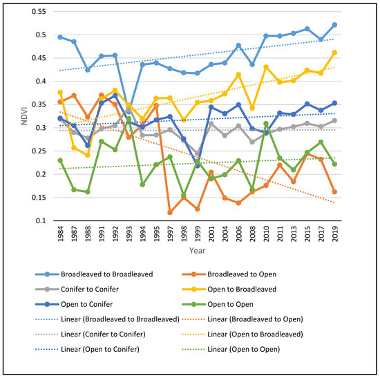
Figure 5.
NDVI multitemporal profile of the main transitions observed in the study area.
4. Discussion
The present study adopted contemporary, time and cost-efficient methods to investigate the long-term vegetation dynamics in a protected area of high conservation value. Identifying environmental parameters extracted from satellite images enables. through geographic information systems. phenomena and processes that until recently required field measurements to be identified and interpreted. As the amplitude of the study period exceeded the duration of operation of one satellite, the retrieval of the images from the last three satellites of the Landsat program was self-evident. However, given the range of time and the aim to achieve compatibility mainly with Landsat 8 OLI/TIRS sensor images, preprocessing was required for a solid analysis, and this is why Level 2 data were employed. Furthermore, the improvement of the contrast of each index image with the method of histogram stretching proved to be very useful. This improved the aesthetics of the images and mitigated the interannual differences in vegetation index values, which did not show changes in vegetation, by smoothing out the sharp fluctuations.
The results clearly demonstrate a significant increase in vegetation cover during the study period. These results seem to be in full agreement with the history of the region but also with its demographic developments. Having lost a large part of its anthropogenic influence for decades due to socio-political and economic changes, a recovery in the area’s vegetation has taken place [54]. Oikonomakis & Ganatsas [54], for part of the study area, reported significant changes between 1945 and 2009 with open habitats decreasing from 50.22% to 3.21% and the extent of forests increasing by 96.79%. Obviously, this forest expansion continues to this day, with probably a decreasing rate since a low percentage of open areas are still being used as pastureland by the few remaining livestock, or they have been degraded to such an extent that it slows down the ecological succession. The main transition observed in this study is from open habitats, with low or no woody vegetation at all, to broadleaved forests. The latter constitute the dominant landcover type during the entire study period. Based on the observation during the fieldwork, the main taxa acting as pioneer species and encroaching the open habitats are Carpinus orientalis Mill., Ostrya caprinifolia Scop., Acer campestre L., A. monspessulanum L., A. pseudoplatanus L., Crataegus monogyna Jacq., Paliurus spina christi Mill. and Rosa sp. At the higher altitudes, where a transition from open habitats to conifer forests occur, the main encroaching species are Pinus nigra and P. silvestris. Land abandonment and the consequent expansion of forested areas is not a neutral event but a dynamic process. It has positive and negative consequences that depend each time on various local conservation priorities, ecological, economic and cultural factors [55,56,57].
Several studies point out the positive effects of the recovery of natural ecosystems as a result of land abandonment and the decrease of human impacts in mountainous areas. Navaro & Pereira [58] consider land abandonment and forest transition a major ecological process that leads to a significant improvement of forests ecological integrity and results in a significant increase in important ecosystem services such as carbon sequestration and recreation [59]. The increase in large mammal populations in Europe is undoubtedly a clear indication that spontaneous land abandonment associated with forest expansion has favored the population of these emblematic species perhaps more than any applied conservation policy [60]. Given that the study area accommodates a high number of large mammals, an increase in their populations is expected and, in fact, has probably already happened since, according to the locals, the incidents of conflicts between large carnivores and livestock has increased. However, no relevant studies have been conducted on the population trends in these species in the study area.
The loss of heterogeneity in this mountainous landscape, on the other hand, has been reported to have detrimental effects on local biodiversity since it affects both species that depend on open habitats for feeding and nesting and species that depend on the abundance of the previous ones. As suggested by Kati et al. [61] landscape heterogeneity can be considered as a surrogate of biodiversity, with increased levels of heterogeneity being related to increased biodiversity. Several studies suggest a negative relationship between loss of open habitats and biodiversity. Farina [62] has found a strong dependence of bird species on the availability of cultivated land in mountainous landscapes and a negative relationship of species richness with proximity to forested areas, while similar results have been reported by Zakkak et al. [63]. Otero et al. [64] has questioned the relationship between land abandonment and ecosystem recovery, pointing out the ecological significance of non-forest habitats and heterogeneity in maintaining biodiversity. The need of maintaining open habitats in primarily forested landscapes for providing suitable habitat for large birds is also pointed out by Xofis & Poirazidis [47] in their study on the landscape dynamics of the Dadia Forest National Park, where the loss of open habitats was associated with the loss of suitable habitats for raptors.
Another important consequence of land abandonment and forest recovery is the increase of biomass, which, on the one hand, is a positive service due to the higher concentration of carbon, but, on the other, is negative because it increases the amount and continuity of fuel [15,65]. This trend has been observed in several other areas with similar vegetation dynamics and, as a result, the relative importance of weather patterns and fuel in determining fire regime and behavior has shifted in recent years in favor of the former, and fires have turned from “fuel-driven” to “weather-driven” [66,67,68,69]. This simply means that when whether conditions are suitable for a wildfire to start and progress, then it is likely to turn into an intense fire because fuel availability is ensured. Furthermore, Konoes et al. [70] reported an increase in the altitudinal range at which fires occur in recent years, demonstrating the increased risk of forest fires in non-fire prone environments, where species are not adapted to frequent fires. A similar observation was made by Xofis & Poirazidis [47] for another protected area in northern Greece, which indicates the increased susceptibility of mountainous areas to wildfires.
There are several other aspects that could be investigated regarding the landscape dynamics of the study area and its consequences on biodiversity and biomass accumulation. The use of Lidar or Laser data could provide useful insights on the biomass increase during the study period and the associated impact on wildfire risk. Furthermore, an analysis of wildlife population trends could also clarify the positive or negative impact of landscape dynamics in this area and probably elsewhere, too.
5. Conclusions
The results of the current study, which used remote sensing data and multiple methods, confirms previously reported results that in the mountainous areas of Europe, due to land abandonment, there is a clear trend towards increasing forest cover and decreasing open habitats and landscape diversity. This trend benefits forest ecosystems by increasing their connectivity and decreasing their fragmentation, with positive consequences for biodiversity and especially for large mammals, carbon sequestration, recreation and other ecosystem services. On the other hand, species that are dependent on open habitats are likely to face population decrease. At the same time, the risk of wildfires is likely to increase due to the increased amount and continuity of fuels. While the positive or negative signing of the observed trend depends on the conservation priorities and local socio-environmental parameters, it is certain that the monitoring of land-use changes, using time and cost efficient manners, over long periods of time is essential for meeting the environmental conservation targets set at policy level. While conserving natural processes such as ecological succession is important for ensuring the ecological integrity of ecosystems, it is also important to plan based on the local peculiarities. The loss of open areas may cause cascade effects, with loss of biodiversity on species depending on open habitats for feeding and/or nesting. As a result, based on the analysis of landscape trends, policy and management interventions may need to be planned in order to ensure maximum protection to and conservation of ecological resources.
Author Contributions
Conceptualization, P.X. and J.A.S.; methodology, P.X. and J.A.S.; software, P.X., J.A.S., S.C. and A.S.C.; validation, P.X., J.A.S. and S.C.; formal analysis, P.X. and J.A.S.; investigation, P.X. and J.A.S.; resources, P.X. and J.A.S.; data curation, P.X. and J.A.S.; writing—original draft preparation, P.X., J.A.S., S.C. and A.S.C.; writing—review and editing, P.X.; visualization, P.X., J.A.S. and S.C.; supervision, P.X. All authors have read and agreed to the published version of the manuscript.
Funding
This research received no external funding.
Conflicts of Interest
The authors declare no conflict of interest.
References
- Diamond, J. Collapse: How Societies Choose to Fail or Succeed; Penguin Books: New York, NY, USA, 2005; p. 575. [Google Scholar]
- Kulakowski, D.; Seidl, R.; Holeksa, J.; Kuuluvainen, T.; Nagel, T.A.; Panayotov, M.; Svoboda, M.; Thorn, S.; Vacchiano, G.; Whitlock, C.; et al. A walk on the wild side: Disturbance dynamics and the conservation and management of European mountain forest ecosystems. For. Ecol. Manag. 2017, 388, 120–131. [Google Scholar] [CrossRef] [PubMed] [Green Version]
- Mantero, G.; Morresi, D.; Marzano, R.; Motta, R.; Mladenoff, D.J.; Garbarino, M. The influence of land abandonment on forest disturbance regimes: A global review. Landsc. Ecol. 2020, 35, 2723–2744. [Google Scholar] [CrossRef]
- Forest Europe. State of Europe’s Forests 2020; Ministerial Conference on the Protection of Forests in Europe—Forest Europe: Bratislava, Slovakia, 2020.
- Dimopoulos, T.; Kizos, T. Mapping change in the agricultural landscape of Lemnos. Landsc. Urban Plan. 2020, 203, 103894. [Google Scholar] [CrossRef]
- Conedera, M.; Colombaroli, D.; Tinner, W.; Krebs, P.; Whitlock, C. Insights about past forest dynamics as a tool for present and future forest management in Switzerland. For. Ecol. Manag. 2017, 388, 100–112. [Google Scholar] [CrossRef] [Green Version]
- Loran, C.; Ginzler, C.; Burgi, M. Evaluating forest transition based on a multi-scale approach: Forest area dynamics in Switzerland 1850–2000. Reg. Environ. Chang. 2016, 16, 1807–1818. [Google Scholar] [CrossRef]
- San Roman Sanz, A.; Fernandez, C.; Mouillot, F.; Ferrat, L.; Istria, D.; Pasqualini, V. Long-term forest dynamics and land-use abandonment in the Mediterranean mountains, Corsica, France. Ecol. Soc. 2013, 18, 38. [Google Scholar] [CrossRef] [Green Version]
- Hadjigeorgiou, I. Past, present and future of pastoralism in Greece. Pastor. Res. Policy Pract. 2011, 1, 24. [Google Scholar] [CrossRef] [Green Version]
- Gidarakou, I.; Apostolopoulos, C. The productive system of itinerant stockfarming in Greece. Medit 1995, 3, 56–63. [Google Scholar]
- Pérez-Hernández, J.; Gavilán, R.G. Impacts of Land-Use Changes on Vegetation and Ecosystem Functioning: Old-Field Secondary Succession. Plants 2021, 10, 990. [Google Scholar] [CrossRef]
- Labaune, C.; Magnin, F. Pastoral management vs. land abandonment in Mediterranean uplands: Impact on land snail communities. Glob. Ecol. Biogeogr. 2002, 11, 237–245. [Google Scholar] [CrossRef]
- Lasanta, T.; Nadal-Romero, E.; Arnáez, J. Managing abandoned farmland to control the impact of revegetation on the environment. The state of the art in Europe. Environ. Sci. Policy 2015, 52, 99–109. [Google Scholar] [CrossRef] [Green Version]
- Ustaoglu, E.; Collier, M.J. Farmland abandonment in Europe: An overview of drivers, consequences, and assessment of the sustainability implications. Environ. Rev. 2018, 26, 396–416. [Google Scholar] [CrossRef]
- Vacchiano, G.; Garbarino, M.; Lingua, E.; Motta, R. Forest dynamics and disturbance regimes in the Italian Apennines. For. Ecol. Manag. 2017, 388, 57–66. [Google Scholar] [CrossRef] [Green Version]
- Keenleyside, C.; Tucker, G. Farmland Abandonment in the EU: An Assessment of Trends and Prospects; Institute for European Environmental Policy WWF: London, UK, 2010; p. 98. [Google Scholar]
- Haddad, N.M.; Brudvig, L.A.; Clobert, J.; Kendi, D.F.; Gonzalez, A.; Holt, R.D.; Lovejoy, E.T.; Sexton, J.O.; Austin, M.P.; Collins, C.D.; et al. Habitat fragmentation and its lasting impact on Earth’s ecosystems. Sci. Adv. 2015, 1, e1500052. [Google Scholar] [CrossRef] [PubMed] [Green Version]
- Koko, A.F.; Yue, W.; Abubakar, G.A.; Hamed, R.; Alabsi, A.A.N. Monitoring and Predicting Spatio-Temporal Land Use/Land Cover Changes in Zaria City, Nigeria, through an Integrated Cellular Automata and Markov Chain Model (CA-Markov). Sustainability 2020, 12, 452. [Google Scholar] [CrossRef]
- European Environment Agency. Streamlining European Biodiversity Indicators 2020: Building a Future on Lessons Learnt from the SEBI 2010 Process; EEA Technical Report No 11; European Environment Agency: Copenhagen, Denmark, 2012.
- Sohl, T.; Sleeter, B. Role of Remote Sensing for Land-Use and Land-Cover Change Modeling. In Remote Sensing of Lend Use and Land Cover: Principles and Applications; Giri, C., Ed.; CRC Press: Boca Raton, FL, USA, 2012; pp. 225–239. [Google Scholar]
- Bannari, A.; Morin, D.; Bonn, F.; Huete, A.R. A review of vegetation indices. Remote Sens. Rev. 1995, 13, 95–120. [Google Scholar] [CrossRef]
- Banskota, A.; Kayastha, N.; Falkowski, M.J.; Wulder, M.A.; Froese, R.E.; White, J.C. Forest Monitoring Using Landsat Time Series Data: A Review. Can. J. Remote Sens. 2014, 40, 362–384. [Google Scholar] [CrossRef]
- Bright, B.C.; Hudak, A.T.; Kennedy, R.E.; Braaten, J.D.; Khalyani, A.H. Examining post-fire vegetation recovery with Landsat time series analysis in three western North American forest types. Fire Ecol. 2019, 15, 8. [Google Scholar] [CrossRef] [Green Version]
- Kibler, C.L.; Parkinson, A.-M.L.; Peterson, S.H.; Roberts, D.A.; D’Antonio, C.M.; Meerdink, S.K.; Sweeney, S.H. Monitoring Post-Fire Recovery of Chaparral and Conifer Species Using Field Surveys and Landsat Time Series. Remote Sens. 2019, 11, 2963. [Google Scholar] [CrossRef] [Green Version]
- Meneses, B.M. Vegetation Recovery Patterns in Burned Areas Assessed with Landsat 8 OLI Imagery and Environmental Biophysical Data. Fire 2021, 4, 76. [Google Scholar] [CrossRef]
- Morresi, M.; Vitali, A.; Urbinati, C.; Garbarino, M. Forest Spectral Recovery and Regeneration Dynamics in Stand-Replacing Wildfires of Central Apennines Derived from Landsat Time Series. Remote Sens. 2019, 11, 308. [Google Scholar] [CrossRef] [Green Version]
- Vogelmann, J.E.; Gallant, A.L.; Shi, H.; Zhu, Z. Perspectives on monitoring gradual change across the continuity of Landsat sensors using time-series data. Remote Sens. Environ. 2016, 185, 258–270. [Google Scholar] [CrossRef] [Green Version]
- Zhu, Z.; Wulder, M.A.; Roy, D.P.; Woodcock, C.E.; Hansen, M.C.; Radeloff, V.C.; Healey, S.P.; Schaaf, C.; Hostert, P.; Strobl, P.; et al. Benefits of the free and open Landsat data policy. Remote Sens. Environ. 2019, 224, 382–385. [Google Scholar] [CrossRef]
- Poirazidis, K.; Bontzorlos, V.; Xofis, P.; Zakkak, S.; Xirouchakis, S.; Grigoriadou, E.; Kechagioglou, S.; Gasteratos, I.; Alivizatos, H.; Panagiotopoulou, M. Bioclimatic and environmental suitability models for capercaillie (Tetrao urogallus) conservation: Identification of optimal and marginal areas in Rodopi Mountain-Range National Park (Northern Greece). Glob. Ecol. Conserv. 2019, 17, e00526. [Google Scholar] [CrossRef]
- Rhodopi Mountain Range National Park. Available online: http://www.fdor.gr/index.php (accessed on 20 November 2021).
- Crist, E.P.; Cicone, R.C. Application of the Tasseled Cap Concept to simulated thematic mapper data. Photogramm. Eng. Remote Sens. 1984, 50, 343–352. [Google Scholar]
- Polevshchikova, I. Disturbance analyses of forest cover dynamics using remote sensing and GIS. IOP Conf. Ser. Earth Environ. Sci. 2019, 316, 012053. [Google Scholar] [CrossRef]
- Rouse, J.W., Jr.; Haas, R.H.; Schell, J.A.; Deering, D.W.; Harla, J.C. Monitoring the Vernal Advancement 1 and Retrogradation (Greenwave Effect) of Natural Vegetation; Remote Sensing Center: Monterey, CA, USA, 1974. [Google Scholar]
- Huete, A.R. A Soil-Adjusted Vegetation Index (SAVI). Remote Sens. Environ. 1988, 25, 295–309. [Google Scholar] [CrossRef]
- Jiang, Z.; Huete, A.R.; Didan, K.; Miura, T. Development of a two-band enhanced vegetation index without a blue band. Remote Sens. Environ. 2008, 112, 3833–3845. [Google Scholar] [CrossRef]
- Gao, B.C. NDWI—A normalized difference water index for remote sensing of vegetation liquid water from space. Remote Sens. Environ. 1996, 58, 257–266. [Google Scholar] [CrossRef]
- Diek, S.; Fornallaz, F.; Schaepman, M.E.; De Jong, R. Barest Pixel Composite for Agricultural Areas Using Landsat Time Series. Remote Sens. 2017, 9, 1245. [Google Scholar] [CrossRef] [Green Version]
- Viedma, O.; Melia, J.; Segarra, D.; Garcia-Haro, J. Modeling rates of ecosystem recovery after fires by using Landstat TM Data. Remote Sens. Environ. 1997, 61, 383–398. [Google Scholar] [CrossRef]
- Volkova, L.; Adinugroho, W.C.C.; Krisnawati, H.; Imanuddin, R.; Weston, C.J.J. Loss and Recovery of Carbon in Repeatedly Burned Degraded Peatlands of Kalimantan, Indonesia. Fire 2021, 4, 64. [Google Scholar] [CrossRef]
- Storey, E.A.; Stow, D.A.; O’Leary, J.F. Assessing postfire recovery of chamise chaparral using multi-temporal spectral vegetation index trajectories derived from Landsat imagery. Remote Sens. Environ. 2016, 183, 53–64. [Google Scholar] [CrossRef] [Green Version]
- Abram, N.K.; MacMillan, D.C.; Xofis, P.; Ancrenaz, M.; Tzanopoulos, J.; Ong, R.; Goossens, B.; Koh, L.P.; Del Valle, C.; Peter, L.; et al. Identifying Where REDD+ Financially Out-Competes Oil Palm in Floodplain Landscapes Using a Fine-Scale Approach. PLoS ONE 2016, 11, e0156481. [Google Scholar] [CrossRef] [PubMed] [Green Version]
- Ceccato, P.; Flasse, S.; Tarantola, S.; Jacquemond, S.; Gregoire, J.M. Detecting vegetation water content using reflectance in the optical domain. Remote Sens. Environ. 2001, 77, 22–33. [Google Scholar] [CrossRef]
- Rikimaru, A.; Roy, P.S.; Miyatake, S. Tropical forest cover density mapping. Trop. Ecol. 2002, 43, 39–47. [Google Scholar]
- Yue, S.; Wang, C. The Mann-Kendall Test Modified by Effective Sample Size to Detect Trend in Serially Correlated Hydrological Series. Water Resour. Manag. 2004, 18, 201–218. [Google Scholar] [CrossRef]
- Trimple. Ecognition Developer Reference Book; Trimble Documentation: Munich, Germany, 2014. [Google Scholar]
- Xofis, P.; Konstantinidis, P.; Papadopoulos, I.; Tsiourlis, G. Integrating Remote Sensing Methods and Fire Simulation Models to Estimate Fire Hazard in a South-East Mediterranean Protected Area. Fire 2020, 3, 31. [Google Scholar] [CrossRef]
- Xofis, P.; Poirazidis, K. Combining different spatio-temporal resolution images to depict landscape dynamics and guide wildlife management. Biol. Conserv. 2018, 218, 10–17. [Google Scholar] [CrossRef]
- Xofis, P.; Tsiourlis, G.; Konstantinidis, P. A Fire Danger Index for the early detection of areas vulnerable to wildfires in the Eastern Mediterranean region. Euro-Mediterr. J. Environ. Integr. 2020, 5, 32. [Google Scholar] [CrossRef]
- Chavez, P.S.; Kwarteng, A.Y. Extracting spectral contrast in Landsat Thematic Mapper image data using selective principal component analysis. Photogramm. Eng. Remote Sens. 1989, 55, 229–348. [Google Scholar]
- Weiers, S.; Bock, M.; Wissen, M.; Rossner, G. Mapping and indicator approaches for the assessment of habitats at different scales using remote sensing and GIS methods. Landsc. Urban Plan. 2004, 67, 43–65. [Google Scholar] [CrossRef]
- Kleinod, K.; Wissen, M.; Bock, M. Detecting vegetation changes in a wetland area in Northern Germany using earth observation and geodata. J. Nat. Conserv. 2005, 13, 115–125. [Google Scholar] [CrossRef]
- Xofis, P.; Buckley, G.P.; Takos, I.; Mitchley, J. Long term post-fire vegetation dynamics in North-East Medi-terranean ecosystems. The case of Mount Athos Greece. Fire 2021, 4, 92. [Google Scholar] [CrossRef]
- Rempel, R.S.; Kaukinen, D.; Carr, A.P. Patch Analyst and Patch Grid; Ontario Ministry of Natural Resources Centre for Northern Forest Ecosystem Research: Thunder Bay, ON, Canada, 2012.
- Oikonomakis, N.; Ganatsas, P. Land cover changes and forest succession trends in a site of Natura 2000 network (Elatia forest), in northern Greece. For. Ecol. Manag. 2012, 285, 153–163. [Google Scholar] [CrossRef]
- Preiss, E.; Martin, J.-L.; Debussche, M. Rural depopulation and recent landscape changes in a Mediterranean region: Consequences to the breeding avifauna. Landsc. Ecol. 1997, 12, 51–61. [Google Scholar] [CrossRef]
- Queiroz, C.; Beilin, R.; Folke, C.; Lindborg, R. Farmland abandonment: Threat or opportunity for biodiversity conservation? A global review. Front. Ecol. Environ. 2014, 12, 288–296. [Google Scholar] [CrossRef]
- MacDonald, D.; Crabtree, J.R.; Wiesinger, G.; Dax, T.; Stamou, N.; Fleury, P.; Gutierrez Lazpita, J.; Gibon, A. Agricultural abandonment in mountain areas of Europe: Environmental consequences and policy response. J. Environ. Manag. 2000, 59, 47–69. [Google Scholar] [CrossRef]
- Navarro, L.M.; Pereira, H.M. Rewilding abandoned landscapes in Europe. Ecosystems 2012, 15, 900–912. [Google Scholar] [CrossRef] [Green Version]
- Prior, J.; Brady, E. Environmental Aesthetics and Rewilding. Environ. Values 2017, 26, 31–51. [Google Scholar] [CrossRef] [Green Version]
- Giapooliti, S.; Brito, D.; Cerfolli, F.; Franco, F.; Krystufek, B.; Battisti, C. Europe as a model for large carnivores conservation: Is the glass half empty or half full? J. Nat. Conserv. 2018, 41, 73–78. [Google Scholar] [CrossRef]
- Kati, V.; Poirazidis, K.; Dufrene, M.; Halley, J.M.; Korakis, G.; Schindler, S.; Dimopoulos, P. Towards the use of ecological heterogeneity to design reserve networks: A case study from Dadia National Park, Greece. Biodivers. Conserv. 2010, 19, 1585–1597. [Google Scholar] [CrossRef]
- Farina, A. Landscape structure and breeding bird distribution in a sub-Mediterranean agro-ecosystem. Landsc. Ecol. 1997, 12, 362–378. [Google Scholar] [CrossRef]
- Zakkak, S.; Radovic, A.; Nikolov, S.C.; Shumka, S.; Kakalis, L.; Kati, V. Assessing the effect of agricultural land abandonment on bird communities in southern-eastern Europe. J. Environ. Manag. 2015, 164, 171–179. [Google Scholar] [CrossRef] [PubMed]
- Otero, I.; Marull, J.; Tello, E.; Diana, G.L.; Pons, M.; Coll, F.; Martí Boada, M. Land abandonment, landscape, and biodiversity: Questioning the restorative character of the forest transition in the Mediterranean. Ecol. Soc. 2015, 20, 7. [Google Scholar] [CrossRef] [Green Version]
- Moreira, F.; Viedma, O.; Arianoutsou, M.; Curt, T.; Koutsias, N.; Rigolot, E.; Barbati, A.; Corona, P.; Vaz, P.; Xanthopoulos, G.; et al. Landscape and wildfire interactions in southern Europe: Implications for landscape management. J. Environ. Manag. 2011, 92, 2389–2402. [Google Scholar] [CrossRef] [Green Version]
- Dimitrakopoulos, A.P.; Vlahou, M.; Anagnostopoulou, C.G.; Mitsopoulos, I.D. Impact of drought on wildland fires in Greece: Implications of climate change? Clim. Chang. 2011, 109, 331–347. [Google Scholar] [CrossRef]
- Koutsias, N.; Xanthopoulos, G.; Founda, D.; Xystrakis, F.; Nioti, F.; Pleniou, M.; Mallinis, G.; Arianoutsou, M. On the relationships between forest fires and weather conditions in Greece from long-term national observations (1894–2010). Int. J. Wildland Fire 2013, 22, 493–507. [Google Scholar] [CrossRef] [Green Version]
- Pausas, J.G.; Fernandez-Munoz, S. Fire regime changes in the Western Mediterranean Basin: From fuel limited to draught-driven fire regime. Clim. Chang. 2012, 110, 215–226. [Google Scholar] [CrossRef] [Green Version]
- Turco, M.; Bedia, J.; Di Liberto, F.; Fiorucci, P.; von Hardenberg, J.; Koutsias, N.; Llasat, M.C.; Xystrakis, F.; Provenzale, A. Decreasing fires in Mediterranean Europe. PLoS ONE 2016, 11, e0150663. [Google Scholar] [CrossRef] [Green Version]
- Kontoes, C.; Keramitsoglou, I.; Papoutsis, I.; Sifakis, N.I.; Xofis, P. National scale operational mapping of burnt areas as a tool for the better understanding of contemporary wildfire patterns and regimes. Sensors 2013, 13, 11146–11166. [Google Scholar] [CrossRef] [PubMed] [Green Version]


Publisher’s Note: MDPI stays neutral with regard to jurisdictional claims in published maps and institutional affiliations. |
© 2022 by the authors. Licensee MDPI, Basel, Switzerland. This article is an open access article distributed under the terms and conditions of the Creative Commons Attribution (CC BY) license (https://creativecommons.org/licenses/by/4.0/).