Article

Spatial Downscaling of Forest Above-Ground Biomass Distribution Patterns Based on Landsat 8 OLI Images and a Multiscale Geographically Weighted Regression Algorithm

1
Co-Innovation Center for Sustainable Forestry in Southern China, Nanjing Forestry University, Nanjing 210037, China
2
College of Forestry, Nanjing Forestry University, Nanjing 210037, China
*
Author to whom correspondence should be addressed.
Forests 2023, 14(3), 526; https://doi.org/10.3390/f14030526
Submission received: 15 February 2023 / Revised: 2 March 2023 / Accepted: 6 March 2023 / Published: 7 March 2023
(This article belongs to the Section Forest Inventory, Modeling and Remote Sensing)

Abstract

:
Forest above-ground biomass (AGB) is an excellent indicator for the health status and carbon sink potential of forest ecosystems, as well as the effectiveness of sustainable forest management practices. However, due to the strong heterogeneity of forest structures, acquiring high-accuracy and high-resolution AGB distributions over wide regions is often prohibitively expensive. To fill the resulting gap, this paper uses part of Lishui city, Zhejiang province as the study area, based on 168 forest sample observations, and proposes a novel integrated framework that combines a multi-scale geographically weighted regression (MGWR) with the co-kriging algorithm to refine the spatial downscaling of AGB. Specifically, optimal predictor variable sets identified by random forest importance ranking, multiple stepwise regression, and Pearson VIF methods were first assessed based on their total explanatory power (R square), followed by reconfirmation of the optimal predictor variable set based on the non-stationarity impact of each variable’s action scale (bandwidth) on the output pattern of AGB downscaling. The AGB downscaling statistical algorithms included MGWR, GWR, random forest (RF), and the ordinary least square (OLS), and their downscaling performances were quantitatively compared to determine the best downscaling method. Ultimately, the downscaled AGB pattern was produced using the best method, which was further refined by considering the spatial autocorrelation in AGB samples by implementing a co-kriging interpolation analysis of the predicted AGB downscaling residuals. The results indicated that the variable set selected by random forest importance ranking had the strongest explanatory power, with a validation R square of 0.58. This was further confirmed by the MGWR analysis which showed that the set of variables produced a more spatially smooth downscaled AGB pattern. Among the set of optimal variables, elevation and aspect affected AGB at local scales, representing a strong spatial heterogeneity. Some textural features and spectral features showed a smooth action scale relative to AGB, showing insignificant spatial scale processes. In the study area with complex terrain, using aspect as a covariant, the co-kriging (CK) model achieved a higher simulation accuracy for the MGWR-predicted AGB residuals than the ordinary kriging model. Overall, the proposed MGWR-CK model, with a final validation R square value of 0.62, effectively improved the spatial distribution characteristics and textural details of AGB mapping without the additional costs of procuring finer satellite images and GIS-based features. This will contribute to the accurate assessment of carbon sinks and carbon stock changes in subtropical forest ecosystems globally.

1. Introduction

Forests convert solar energy into biomass and chemical energy through photosynthesis, while releasing large amounts of oxygen through respiration. Thus, forests play essential roles as “biological pumps” and “buffers” in the carbon cycle between terrestrial ecosystems and the atmosphere [1]. Forest above-ground biomass (AGB) is an important indicator of the productivity of forest ecosystems, and can be used to evaluate carbon stocks and carbon sink potential, as well as being useful in estimating the carbon emissions caused by land use and climate change [2]. Further, long-term monitoring of AGB spatial distributions can help us to understand the consequences of global climate change and to formulate targeted sustainable forest management strategies [3]. Although traditional forest AGB field investigations are highly accurate, they are time-consuming, labor-intensive, costly, destructive, and less feasible on remote and steep slopes [4], therefore it is hard to provide explicit spatio-temporal AGB distribution information for large regions worldwide. Additionally, field inventory methods cannot provide results quickly, and hence cannot support time-sensitive decision making [5]. Therefore, remote sensing images have been identified as a promising alternative when predicting AGB because they provide an abundance of spectral and textural information, fine scale temporal and spatial resolutions, wide coverage, and rapid returns [6]. In fact, during recent decades, combining remote sensing data with the limited available ground-sampling data to map AGB has become a mainstream research direction in the quantitative inversion of forest AGB [7,8].
The sources of remote sensing data vary in their applicability to the quantitative estimation of AGB due to various limitations which can interfere with temporal and spatial scales, and with analytical processes. Moderate and high-resolution remote sensing images are often used for AGB estimations at local and regional scales, and the most commonly used optical remote sensing images include Landsat TM/ETM/OLI [9], MODIS [10], Sentinel-2 [11], GF-2 [12], etc. High-spatial-resolution remote sensing data from unmanned aerial vehicles (UAV) are also used for small-scale AGB estimation [13]. For national- or even global-scale AGB estimations, remote sensing data with lower spatial resolutions are mostly used, but this means that estimation results have relatively low accuracies [7] and cannot reliably represent the spatial details of AGB due to the mixed pixel effects in highly fragmented forest–non-forest fringe landscapes.
Due to the apparent spatial heterogeneity and non-stationarity in AGB, and differences in remote sensing data types and estimation methods, the applications of different sources may produce different random or systematic errors in the AGB estimation process [14]. For example, spatial differences (or scale mismatch) between in-situ sample plot size and remotely sensed image pixel size may lead to AGB estimation errors [15,16]. Næsset et al. argued that, in order to improve the accuracy of AGB estimation, sample size should be taken into account when using remotely sensed data for AGB estimation [17]. Réjou-Méchain et al. used a large-scale global dataset to show that local spatial variability led to large sampling errors when using standard sizes to estimate AGB over large areas [18]. Thus, to obtain more reliable and higher spatial resolution AGB distribution maps from easily accessible, low-cost, and low-resolution remote sensing images, a spatial downscaling operation can be used without additional financial investments to facilitate higher spatial resolution analyses.
Downscaling transforms low-resolution information into high-resolution information and has been notably applied to research on climate change [19], precipitation [20], and ecosystem carbon cycling [21]. Currently, three methods are commonly used for downscaling remote-sensing-based results, comprising statistical downscaling, modulation-assignment-based downscaling, and spectral-mixture-analysis-based downscaling. Among them, statistical downscaling is most widely used due to its ease of operation and satisfactory accuracy [22]. Statistical downscaling is generally implemented by first using established empirical relationships between target variables and strongly related predictor variables at coarse scales [23] and then, based on the core hypothesis of “relational scale invariance” [24], applying the established empirical relationships to the same set of predictors again, but with a finer resolution to generate finer prediction results of the target variables. To date, downscaling studies focusing on forest AGB have been rare. A few studies have used forest vegetation distribution maps to provide representative biomass values for different vegetation types, and downscaled them to a grid to give the average biomass of each vegetation type at large scales to obtain high-resolution biomass data [25]. Obviously, this type of downscaling method is typically based on modulation assignments rather than statistical downscaling. Linear regression models were widely used in early studies of AGB estimation, but they are unable to describe the complex non-linear relationships between AGB and remotely sensed features [26]. In recent years, machine learning models such as artificial neural networks (ANN) [27], support vector machines (SVM) [28], and random forests (RF) [2] are used to simulate the non-linear relationship between AGB and the predictor variables of interest, enabling reliable downscaling from low-resolution to higher-resolution. To date, most of these methods have been used to establish relationships between AGB and various surface physical parameters at global or national scales, ignoring local features of the relationships between parameters [29,30]. However, patterns observed at small scales are often very different from those at larger scales [31].
In the fields of geography and spatial data analysis, instability in the relationships between spatially distributed variables is known as non-stationarity. It has been found that non-stationarity exists in the spatial relationships between satellite data and forest structural characteristics, including net primary productivity and leaf area index [32,33]. Influenced by the interactions among individuals, populations, and the environment, AGB often shows autocorrelation and non-stationarity in its spatial distribution. However, the machine learning model mentioned above does not take into account the effect of spatial non-smoothness on AGB prediction when estimating the AGB. In the field of spatial modelling, several statistical techniques have been developed to model spatially varying relationships between variables [34]. In recent years, as an optimized version of the geographically weighted regression (GWR) model, the multi-scale geographically weighted regression model (MGWR) has been proposed. The MGWR is a powerful extension of GWR; it not only reveals spatial heterogeneity patterns, it measures the operational scales of predictor variables and determines which variables have fixed effects or varying effects over a given study area [35,36].
As mentioned above, many studies have applied downscaling methods in the fields of surface temperature and precipitation [19,20,37], however the statistical downscaling of low-resolution AGB using high-resolution multispectral data has rarely been investigated, especially MGWR-based modelling, which is a relatively unexplored area in the field of remote sensing in forestry studies. Furthermore, most existing AGB prediction models do not adequately account for the differences in the scaling effects among different predictor variables on the spatially divergent patterns of AGB. Thus, the current work developed a framework that integrates MGWR and co-kriging interpolation to adequately account for the complexity (non-stationarity and spatial-autocorrelation) of AGB spatial distributions with the ultimate goal of achieving AGB downscaling based on Landsat OLI images, which acts as the major contribution of the current work to forestry remote sensing. This effort is expected to provide a methodological reference for the generation of fine scale distribution patterns of AGB in areas with complex terrain.

2. Materials and Methods

2.1. Study Area

The study area was located in Lishui City of Zhejiang Province, Eastern China, spanning from 119°7′ E, 28°34′ N to 119°50′ E, 27°31′ N, and included a municipal district, a county-level city, and three counties, with a total area of about 5000 km2 (Figure 1). The major mountains of the study area belong to the Wuyi Mountain System, with topography sloping from southwest to northeast. Lishui is in the Central Subtropical Monsoon Climate Zone, with an annual average temperature of about 17.9 °C, a minimum average of 6.7 °C in January and a maximum average of 28.4 °C in July. The Central Subtropical Monsoon Climate is characterized as having four distinct seasons, warm winters and early springs, abundant precipitation, and co-occurrent rain and hot weather. Lishui possesses rich forest resources and its forest coverage rate was 80.79% in 2013. The dominant tree species are Pinus massoniana Lamb., Cunninghamia lanceolata (Lamb.) Hook, and Cyclobalanopsis glauca (Thunb.) Oerst [38]. However, due to the frequent occurrence of natural disasters and long-term human activities in the area, most of the primary vegetation has been repeatedly modified and used, and the existing vegetation is dominated by secondary and artificial vegetation.

2.2. Data and Preprocessing

2.2.1. Field Data

The ground forest plot inventory data used in this study were compiled from the 2014 National Forest Inventory (NFI) of Zhejiang Province. The NFI of Zhejiang Province started in 1979 when a series of square sample plots with sample areas of 0.08 ha (28.28 m × 28.28 m) were set up using a systematic sampling method. The AGB of each plot was derived by totaling each tree’s measured AGB within a plot, which was calculated using tree-species-specific allometric equations [39]. For certain tree species without available biomass allometric equations, equations for the same genus or family were used as approximate substitutes. To obtain more accurate inversion results, 11 sample plots covered by cloud pixels in the Landsat 8 OLI image were excluded from the analysis. In addition, although the pixel size of OLI images (nominally 30 m × 30 m) gets very close to the size of each sample plot (28.28 m × 28.28 m), there is still a small difference in spatial scale; therefore, to facilitate the modelling and mapping processes, it was necessary to convert the per unit area AGB into the pixel-level AGB, using the unit t/900 m2 [40]. Once done, the SPSS software (version 21.0, Armonk, NY, USA) was used to analyze the statistical characteristics of the post-filtering samples’ AGB values, and those AGB values greater than or less than the global AGB mean plus or minus three times the standard deviation were considered outliers and excluded from further analysis. Ultimately, a total of 168 sample plots were retained, 70% of which were randomly selected for model training and the remaining 30% for model validation. Table 1 summarizes the statistical characteristics of the final sample plots’ AGB values.

2.2.2. Remote Sensing Data and Preprocessing

Two Landsat 8 OLI images with WRS-2 path/row numbers of 119/040 and 119/041, and cloud coverages of 6.89% and 4.02% respectively, acquired on July 22nd 2014, were collected. Additionally, this study used a free digital elevation model (DEM) with a resolution of 30 m (available online: http://earthexplorer.usgs.gov, accessed on 21 November 2021), and derived slope and aspect information through the ArcGIS10.3 package 3D Analyst Tools to support subsequent modelling analysis. Based on the DEM, the Landsat 8 OLI images were ortho-rectified using the RPC workflow embedded in the ENVI 5.3 package to further refine the location accuracy of pixels in the study area by minimizing the effect of terrain relief. At the request of the user when placing the data order, Landsat 8 OLI surface reflectance data can be directly generated from the Landsat Surface Reflectance Code internal program (LaSRC) by the USGS EROS Data Center, which uses MODIS auxiliary climate data and a unique radiative transfer model for aerosol inversion testing using the coastal aerosol belt [41]. Further, topographic correction of the Landsat surface reflectance images was conducted using a C correction model to minimize the effects of terrain shadows on pixel reflectance [42].

2.3. Independent Variable Extraction and Image Fusion

2.3.1. Development of Dependent Variables

In this work, we extracted four types of modelling variables using ENVI 5.3 and ArcGIS 10.3 software. These included original bands and their transformations, vegetation indices, textural features, and topographic features (Appendix A, Table A1). The spectral feature transformations included the principal component analysis (PCA), tasseled cap transformation (TC), and minimum noise fraction (MNF) results, which were implemented to remove redundant information among the original bands, and to generate those integrated features that are potentially highly relevant to AGB. Specifically, three new orthogonal features with clear physical meanings, namely TCB (brightness), TCG (greenness), and TCW (wetness), were generated from the TC transformation to more effectively describe the vegetation statuses [43]. Orthogonal features that retained most of the variances of the original bands were generated using the PCA and MNF. Appendix A, Table A1 provides the technical details of generating the features, of which there were 138 in total to be involved in the modelling analysis.

2.3.2. Image Fusion

To obtain a higher resolution prediction variable set to support the subsequent downscaling modelling, image fusion methods including the Brovey transform [44], GS transform [45], NNDiffuse method [46], and PCA fusion [47] were implemented to blend the panchromatic bands with those spectrally corresponding multi-spectral bands to generate new fused multi-spectral images at a spatial resolution of 15 m. The fusion effect was quantitatively evaluated using the standard deviation, correlation coefficient, average gradient, and information entropy measures to determine the optimal fusion method. Using the optimal method, those features with spatial resolutions of 15 m to be potentially included in the downscaling model were accordingly generated from the fused images and the resampled DEM.

2.4. Determination of Variable Set

Variable selection refers to the determination of the explanatory variables that are most closely related to AGB values using specific criteria, while simultaneously removing redundant variables from the modelling process. To compare the overall relevance of different features or variable combinations to AGB, three variable selection methods, including multiple stepwise regression, random forest importance ranking, and the Pearson correlation coefficient coupled with the variance inflation factor, were implemented and compared.

2.4.1. Multiple Stepwise Regression (MSR)

The multiple stepwise screening method combines the advantages of the forward and backward selection of variable methods by building a separate one-dimensional regression model with the dependent variable and calculating the F value for each variable. When building the stepwise regression model, the independent variable with the highest F value among the predictor variables not currently included in the model is selected for inclusion in the model. Then, a t-test is conducted on each of the selected predictor variables and if there are any selected predictor variables that are no longer significant, they are removed. The above steps are repeated until no more significant explanatory variables are selected for inclusion in the regression equation and no more insignificant explanatory variables are removed from the regression equation, at which point the subset retained is considered optimal and used as the characteristic variables for building the model [48]. The method has been proven to be effective in the selection of AGB modelling variables [49]. In this analysis, stepwise regressions were performed in the SPSS software (Version 25, Armonk, NY, USA), and the significance levels of the F-test for variable entry and removal were set to 0.05 and 0.10, respectively.

2.4.2. Random Forest Importance Ranking (RFR)

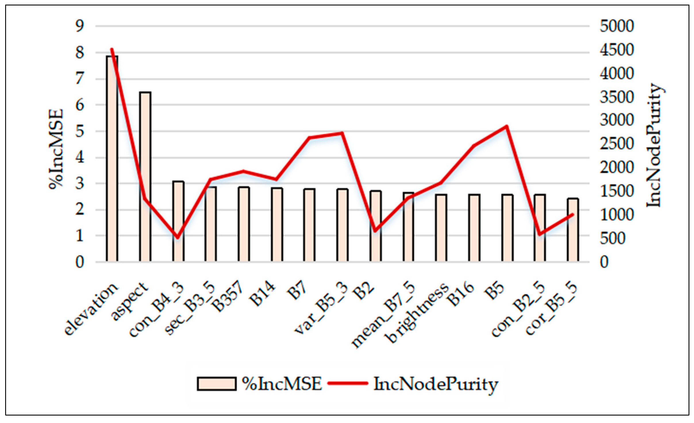
The random forest importance ranking algorithm was used to perform feature importance comparisons to select the predictors with high importance. The random forest algorithm uses two metrics for measuring the importance of variables. The first metric (calculated from the ranking of the out-of-bag data) is the increase in the percentage of mean square error (%IncMSE) of the predictions for each tree, and the second metric is the total reduction in increased node purity (IncNodePurity) from the split of the average variable over all the trees. Higher %IncMSE and IncNodePurity values indicate the predictor variables are more important [50].

2.4.3. Pearson Correlation Coefficient (Pearson VIF)

The Pearson correlation coefficient was used to identify the characteristic variables with high correlations to AGB. These variables were then tested for multicollinearity, which was judged using the variance inflation factor (VIF) in this study:
V I F = 1 / 1 R i 2 ,   i = 1 , 2 ,   , k
where R i is the complex correlation coefficient of the i th variable on the remaining k-1 predictive variables. There is no multicollinearity if VIF ranges from 0 to 10, but high multicollinearity exists between variables if VIF  10, indicating that some of them should be removed from the model [51].

2.5. Multiscale Geographic Weighted Regression (MGWR)

Fotheringham et al. [52] proposed the MGWR model, which was further improved by Yu et al. considering the local parameter statistical inference [53]. Compared to the classical GWR, the MGWR has the advantage of generating processes that more closely reflect the actual state-space processes by not assuming there is a single bandwidth scale for all variables. MGWR can be applied to investigate various influential factors and their corresponding processes by considering spatial heterogeneity and operational scale [54]. Theoretically, MGWR allows different spatial scales for different predictors, indicating that each predictor has a different spatial smooth range. In the MGWR model, these spatial smooth ranges are reflected in the bandwidths of the predictors [22]. A small bandwidth means that the relationship varies at a relatively small scale, while a bigger bandwidth indicates that the relationship varies at a larger scale. A bandwidth that is closer to the global domain represents a higher degree of spatial smoothness and indicates that the predictor variable produces results with less variability in the study area [54]. MGWR transforms the classical GWR fixed-bandwidth model into a multi-bandwidth model and uses a back-fitting algorithm to calculate each predictor’s scale of influence. In this work, MGWR was applied to capture the differences in the spatial heterogeneity among the various predictor variables. The MGWR model is expressed as follows:
y i = j = 1 k β b w j u i , v i x i j + ε
where y i is the ith observation value of the response variable; x i j is the observation value of the j th explanatory variable at location i ; β b w j represents the regression coefficients of different variables j at different bandwidths; u i , v i are the geographic coordinates of the sample point; k represents the number of predictor variables; and ε is the model regression residual.
To construct a downscaled relational model between AGB and the set of predictor variables, this analysis used the open source software MGWR2.2 and the mgwr site package in the Python environment [55]. In order to compare different bandwidths obtained from the MGWR model, it was necessary to standardize the dependent and independent variables so that they were centered at zero and based on a same range of variation [55]. During the model construction process, the most commonly used quadratic kernel function and the bandwidth selection criterion (the corrected Akaike information criterion (AICc)) were applied, and the search for the optimal bandwidth was conducted using the golden partition algorithm. All the open source packages were provided by the School of Geographic Sciences and Urban Planning at Arizona State University.

2.6. Model Comparison

To test the performance of the MGWR algorithm (Equation (2)), we compared its analytical results with those of the random forest model (RF), GWR, and the traditional ordinary least squares regression (OLS) method. The classic GWR and OLS models were constructed using the GWR4 package (available online: https:/lsgsup.asu.edu/sparc/gwr4, accessed on 15 September 2021). The random forest (RF) algorithm, proposed by Breiman in 2001, is a machine learning model which is an extension of the Classification and Regression Tree (CART) algorithm that improves the accuracy and stability of the CART model. Each tree in a random forest relies on the values of a randomly selected subset of input variables that are independently sampled, where all trees have the same distribution [56,57]. The implementation of RF depends on the regularization and stopping parameters of the decision tree [58]. RF has multiple notable advantages over other methods: it can easily deal with the non-linear relationships between AGB and various predictors, is insensitive to multicollinearity, and it can effectively prevent over-fitting [59,60]. The construction of the RF model was implemented in the R Studio (Version 4.2.0) platform randomForest package, and three important parameters were tested, namely the number of split variables (mtry; i.e., the number of variables used for splitting, which is determined by random features on each tree node), the number of trees (ntree), and the minimum sample number of terminal nodes (nodesize) [61]. After multiple tries, we used the following values for the parameters: mtry = 4, ntree = 1000, and nodesize = 5 in the current analysis.

2.7. AGB Downscaling

2.7.1. MGWRD Model

The MGWR model can analytically determine the spatial scale of action or the respective bandwidth of each predictor variable, and determine the best combination of predictor variables based on the spatial smoothness of the predicted results. When predictor variables vary less spatially, or have larger scales of action (bandwidths), their effects will be spatially similar with little heterogeneity. This will produce smoother downscaled output results, as shown in Figure 2b. Conversely, more heterogeneous downscaled results will be produced when predictor variables with smaller scales of action (bandwidths) are included, as shown in Figure 2a. Once the optimal combination of predictor variables was determined, the MGWR statistical regression model constructed using coarse datasets (30 m resolution) was directly applied to the set of 15 m resolution predictor variables to fulfill accomplish downscaling. The AGB downscaling process can be written as in Equation (3):
A G B high O V = M G W R D O V
where A G B high denotes the AGB prediction value at the fine scale; O V denotes the optimal set of predictor variables identified by MGWR analysis; and M G W R D denotes the statistical regression model of AGB created from the optimal set of predictor variables with coarser resolutions.

2.7.2. MGWRD-OK and MGWRD-CK Models

Since the MGWRD model does not consider the spatial autocorrelation of the AGB samples, we used a combination of MGWRD and kriging interpolation to more accurately determine the spatial distribution of AGB. The kriging interpolation method used in this paper included both ordinary kriging (OK) and co-kriging (CK) with aspect as the covariant. The specific steps were as follows: (1) the structured components of the 15 m resolution AGB residuals derived from the MGWRD model were separated using the ordinary kriging and co-kriging interpolations, and (2) the separated components were overlaid onto those spatially corresponding the MGWRD predicted AGB values to create a 15 m final AGB distribution pattern. Equations (4) and (5) illustrate the specific rationale of the two steps:
R x i = A G B x i A G B M G W R D x i
A G B M G W R D O K / M G W R D C K x i = A G B M G W R D x i + R O K / C K x i
where R x i is the AGB residual value at sample location i; A G B x i is the observed value of AGB at sample location i; A G B M G W R D x i is the MGWR-predicted value of AGB at sample location i; A G B M G W R D O K / M G W R D C K x i is the predicted value of AGB obtained through the MGWRD-OK or MGWRD-CK models; and R O K / C K x i is the structural component of the residual value interpolated by OK or CK at sample location i. Here we focused on comparing the accuracy of the residual predictions using ordinary kriging (OK) interpolation and co-kriging (CK) interpolation with aspect as the covariate. The semi-covariance function models used in this paper included the exponential models, the spherical models and the Gaussian model. These analyses were implemented using the geostatistical software GS+ (Version 9) and ArcGIS 10.3 software.

2.8. Cross-Validation

Here, the ten-fold cross-validation approach was used to evaluate the mean predictive performances of the four models based on the different predictor variables [62]. Using these calculations, statistics including the mean absolute error (MAE) (Equation (6)), root mean square error (RMSE) (Equation (7)), mean of the coefficient of determination (R2) (Equation (8)), and Bias (Equation (9)) were derived from the ten-fold cross-validation replications to represent the model performances.
M A E = 1 n i = 1 n y ^ i y i
R M S E = 1 n i = 1 n y ^ i y i 2
R 2 = 1 i = 1 n y ^ i y i 2 i = 1 n y ^ i y ¯ 2
B i a s = i = 1 n y ^ i y i n
where n is the total number of the validation observations; y ^ i is the AGB predicted by the model; y i is the observed AGB on the ground; and y ¯ is the arithmetic mean of all observed AGB values.
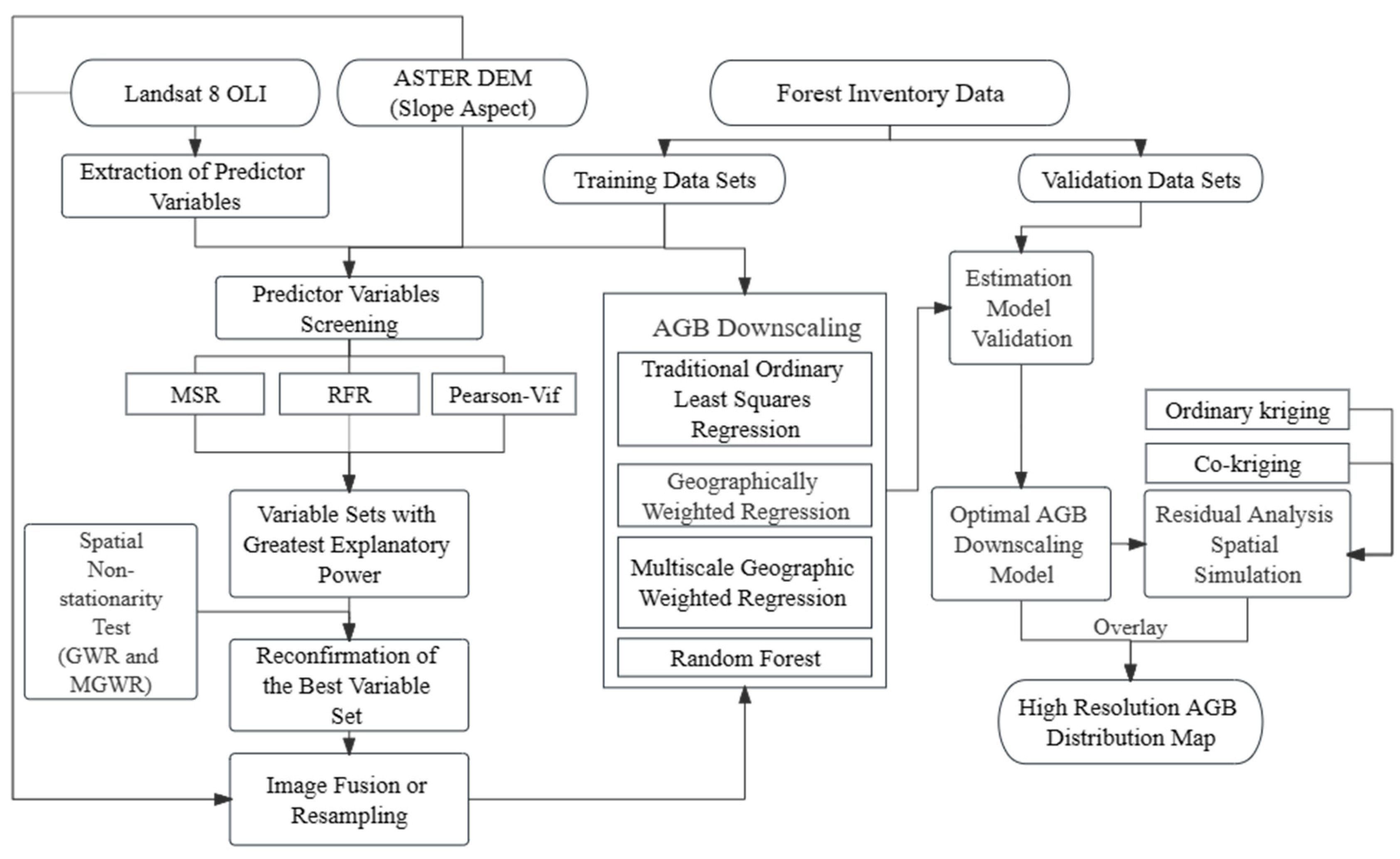
Figure 3 shows the flowchart of the analysis.

3. Results

3.1. Evaluation of Image Fusion Effects

Appendix A, Table A2 provides the quantitative assessment results of the four image fusion methods. Overall, the PCA fusion method gave the best fusion results because it generally had higher correlation coefficient (0.94) and information entropy (8.32) measurements than the other three fusion methods (Appendix A, Table A2). Thus, the PCA-based fused images with spatial resolutions of 15 m were used as the basis from which to extract the sets of potential predictor variables.

3.2. Determination of Predictor Variable Sets

3.2.1. Multiple Stepwise Regression (MSR)

Table 2 summarizes the predictor variables selected by MSR and the corresponding fitted regression equations. MSR ultimately retained 12 predictor variables, among which textures dominated, but spectral characteristics and terrain variables including slope and aspect were also selected.

3.2.2. Random Forest Importance Ranking (RFR)

Figure 4 shows the importance scores of the first 15 variables after 100 runs of the RF model. Based on the comparison of the %IncMSE and IncNodePurity metrics, con_B4_3, B2, and con_B2_5 were removed from the top 15. Finally, the variables elevation, aspect, sec_B3_5, B357, B14, B7, var_B5_3, mean_B7_5, brightness, B16, B5, and cor_B5_5 were selected as input variables for subsequent analysis.

3.2.3. Pearson Correlation Coefficient (Pearson VIF)

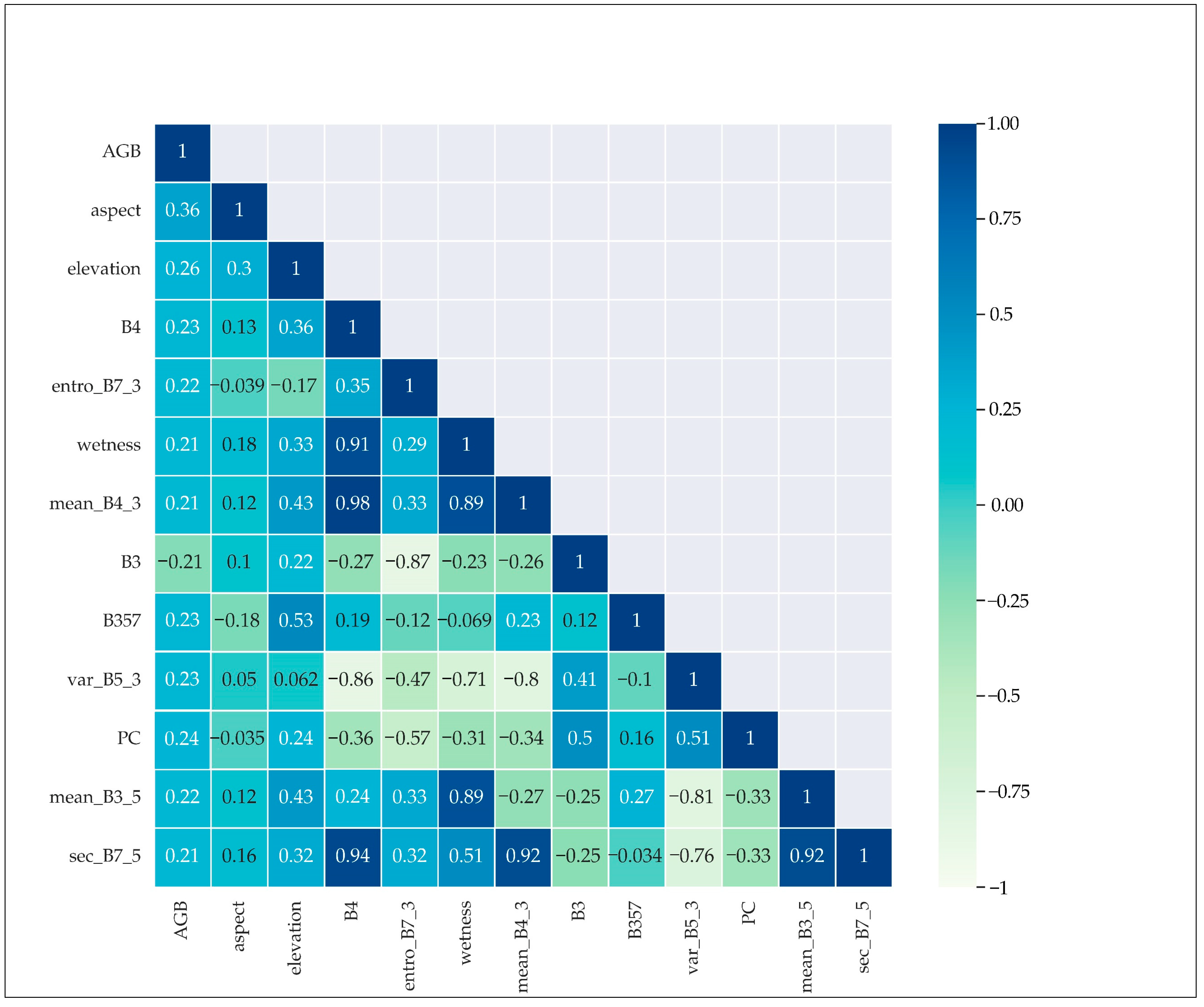
Figure 5 shows the heat map of the Pearson VIF correlations between the AGB and the top 12 predictor variables, including two topographic factors, five texture features, and five spectral features. Of these, the two terrain factors, aspect and elevation, had the strongest correlations with AGB, while the remaining predictor variables did not differ significantly from each other in terms of their correlations with AGB.
By comparing the three sets of selected variables, it was found that the three methods had selected different variables. However, the topographic factors were selected by all three variable screening methods and always ranked in the top three, indicating that they were highly important to AGB estimation. The majority of the other selected features were texture features and combined operation results between bands, followed by a small number of vegetation indices. Specifically, all the three methods regarded aspect as having the strongest response to AGB.

3.3. Scale of Action

Before constructing the MGWR model, a test for spatial autocorrelation among the samples was conducted to determine whether there were significant relationships or not. Based on the test, the MoranI index was 0.23, with a Z-Score of 3.6 and p-value of 0.0003. The Z-score and p-value results jointly indicated that the AGB within the study area exhibited a statistically significant aggregation pattern and was not randomly distributed.
Table 3 shows the different predictive performances of the four AGB downscaling modelling algorithms when applied to the three sets of predictor variables. Compared to the other two variable selection methods, the RFR selected variable set had the lowest RSS, AIC, AICc, and CV values when implementing the OLS, GWR, MGWR, and RF regression analyses and, correspondingly, the goodness of fit (R square value) of the RFR-selected set of variables was the highest (Table 3). Therefore, it was concluded that the variable set selected by RFR was the optimal combination of variables and had the highest explanatory power for the variation in AGB. Furthermore, when using this variable set, the MGWR regression performance was better than those of OLS, GWR, and RF in terms of RSS, AIC, AICc, CV, and R square statistics (Table 3). Thus, it was further concluded that MGWR regression was the best for the current analysis.
Figure 6 shows the scales of action or bandwidths identified by GWR and MGWR for the different predictor variables. Clearly, the classical GWR produced the same bandwidth for all involved variables in each variable set; it could be explained as a weighted average of multiscale effects [52]. In the different independent variable sets, the bandwidths identified by the classical GWR at 121 km, 124 km and 130 km respectively. This assumes that all variables affecting the AGB act on the same regional scale, which imposes significant limitations on the results. In contrast, MGWR can capture differences in the spatial heterogeneity levels of different predictor variables. In Figure 6a, for example, elevation and aspect, had smaller bandwidths, indicating they affected AGB on relatively local scales. Furthermore, on a local scale, the relationships between AGB and the six variables sec_B3_5, NDVI, var_B5_3, B7, mean_B4_5, and B16 exhibited spatial smoothness, but that differed on a broad regional scale. The other variables affected the AGB on global scales, as their optimal bandwidths were near the maximum possible number of neighbors 168 (the entire sample size). The RFR-selected predictor variable set exhibited a larger scale of action, with an average bandwidths and median bandwidths of 130 km and 139 km, respectively, which were closer to the global domain or the total sample size than the others (Figure 6a). These results further confirmed that the RFR-selected predictor variable set was the best and produced less spatially heterogeneous downscaling results.

3.4. MGWRD Model

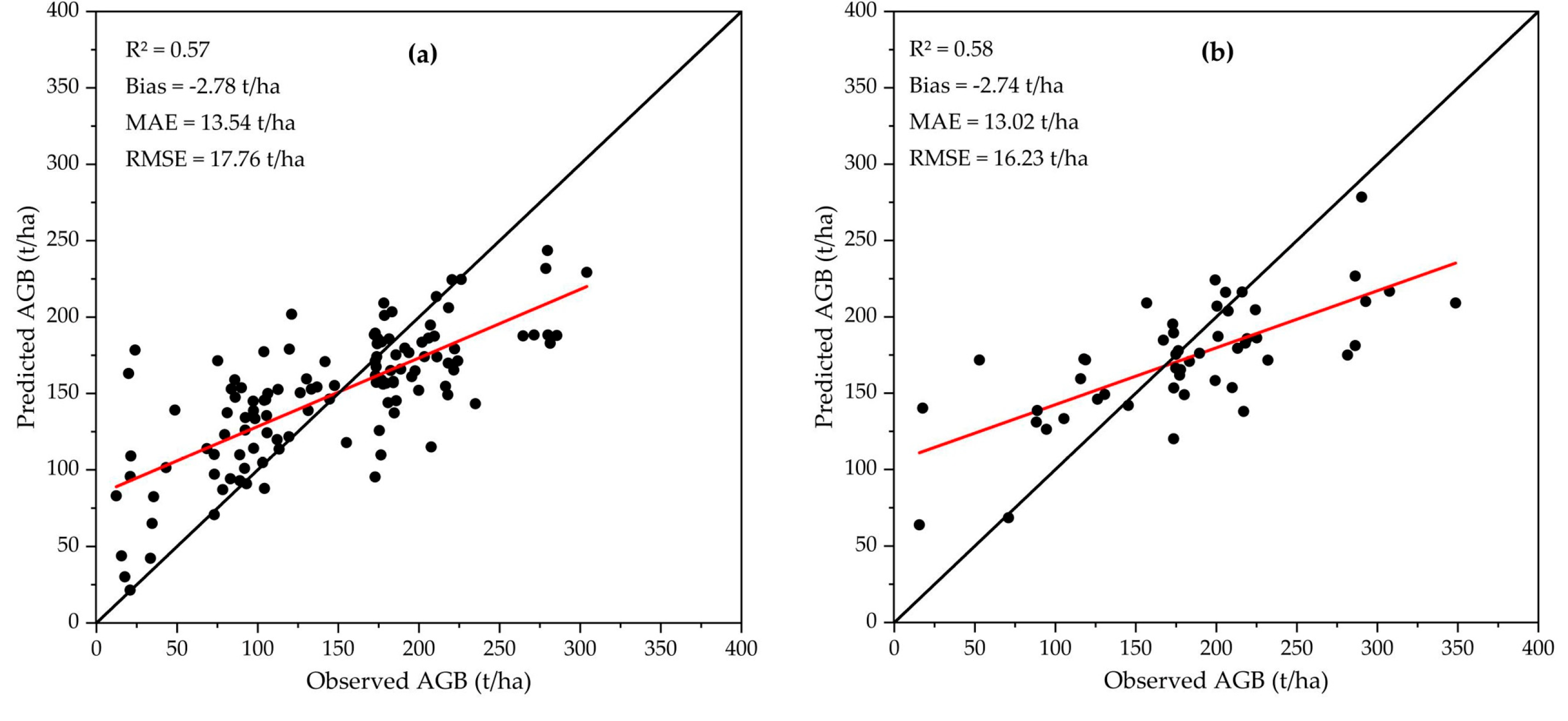
The ten-fold cross validation strategy was used throughout this analysis. Figure 7a,b show the fit accuracy and validation accuracy of the established MGWRD model based on the RFR selected variables. As shown in Figure 7, the fitting accuracy and validation accuracy (R2) of the MGWRD model were 0.57 and 0.58, respectively; the Bias values were −2.78 t/ha and −2.74 t/ha, respectively. This indicated that the MGWRD model constructed in this study had no overfitting effect and achieved a relatively high AGB estimation accuracy. However, Figure 7a,b also show that there was a clear underestimation of the observed high values and an overestimation of the observed low values in the MGWRD-predicted results of AGB.
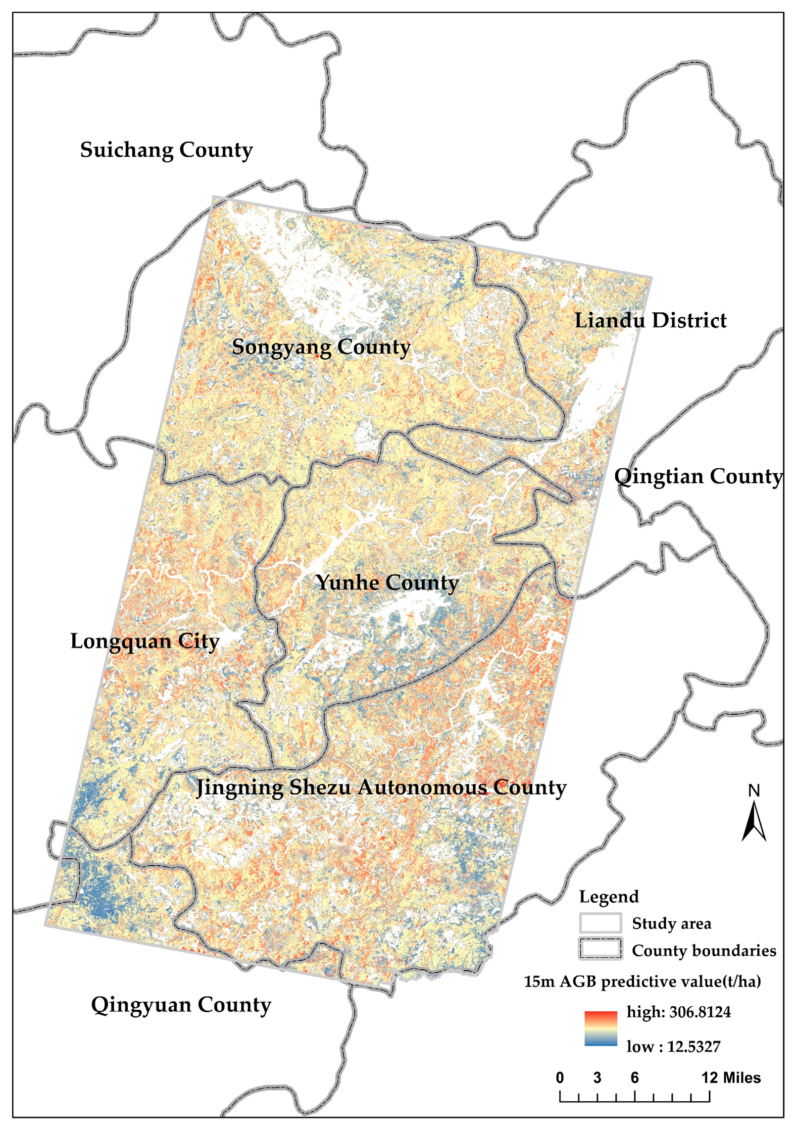
Figure 8 shows the MGWRD-predicted spatial distribution pattern of AGB. The predicted AGB values ranged from 12.53 to 306.81 t/ha. The lower predicted AGB values were mainly distributed in the north, southwest, southeast, and central part of the study area, and the predicted high values were principally concentrated in the south, mid-east, and mid-west regions of the study area.

3.5. MGWRD-CK Model

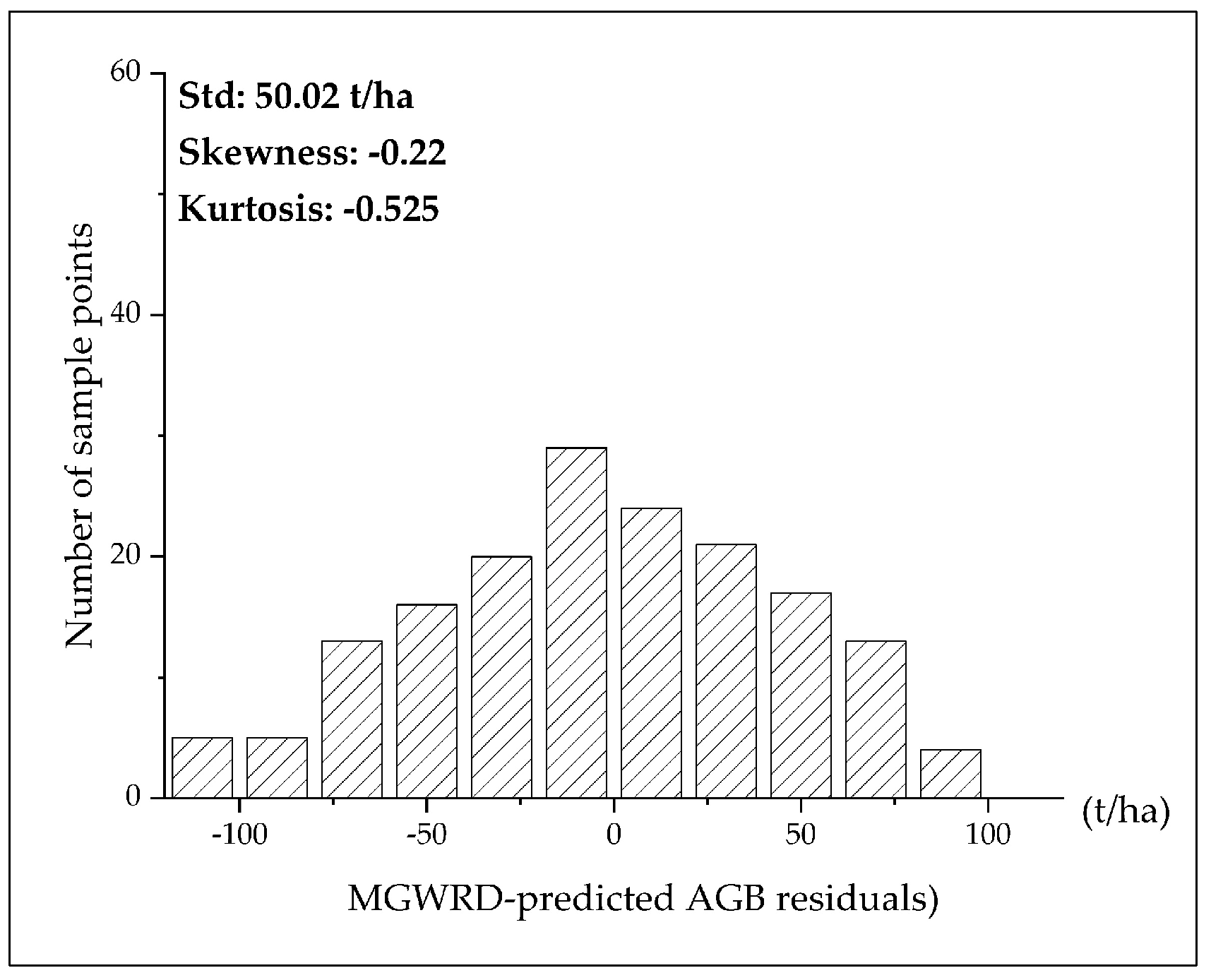
Figure 9 shows a histogram of the MGWRD-predicted AGB residuals. The standard deviation of the residuals was 50.02 t/ha, the absolute kurtosis value was −0.525, and the absolute skewness was close to 1, indicating that the residuals made an approximately normal distribution. Therefore, the prerequisite assumptions for performing kriging interpolation were satisfied and the AGB prediction residuals could be subjected to the subsequent kriging interpolation analysis. The scales of action of all three characteristic variable sets shown in Figure 6 reveal that aspect exhibits a strong spatial heterogeneity and, therefore, was chosen as a covariate in the co-kriging analysis.
Table 4 shows the simulation result residuals and related statistics based on the semi-variance exponential, spherical, and gaussian models via OK and CK simulation strategies, respectively. Based on the results of GS+ modelling, overall, the exponential model outperformed the other two models in both OK and CK simulation strategies, and the exponential model achieved the highest accuracy in the CK simulation, e.g., R square of 0.81 (CK) over 0.78 (OK) (Table 4). Thus, the CK-exponential model was determined to have the best fit for modifying the MGWRD-predicted AGB values to improve the final accuracy of the downscaled AGB.
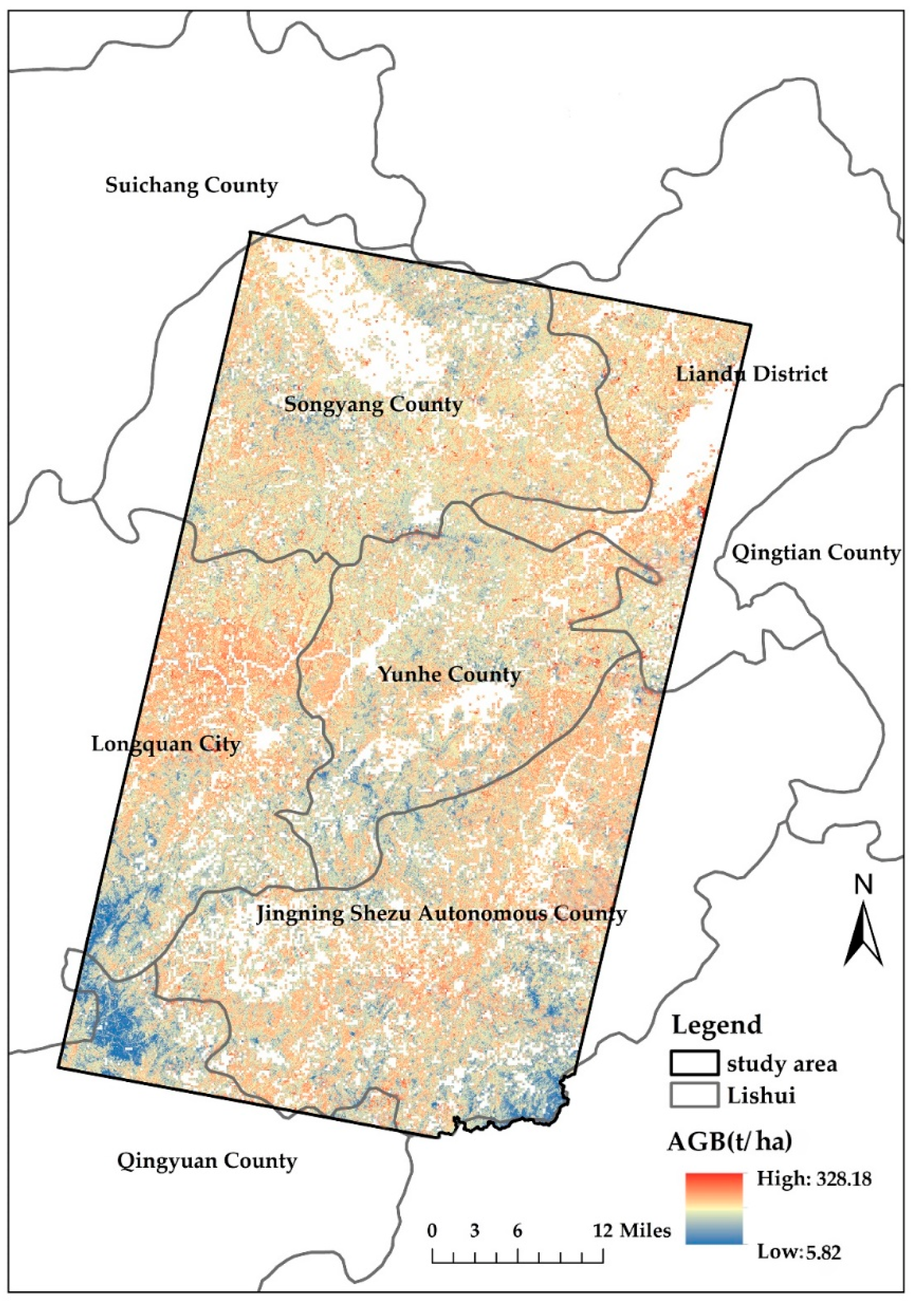
Figure 10 shows the improved AGB predictions based on the MGWRD-CK model. Obviously, there was clear spatial similarity between the MGWRD-CK predictions (Figure 10) and the MGWRD predictions (Figure 8), but in the MGWRD-CK predictions the minimum AGB dropped to 5.82 t/ha and its maximum AGB increased to 328.18 t/ha. Compared to the predictions of the MGWR model, the dynamic range of AGB predictions from MGWRD-CK model was extended, indicating a greater adaptability for AGB prediction. The models were validated using 30% of the independent samples, and the related statistics are summarized in Table 5. The accuracy was better in the MGWRD-OK and MGWRD-CK models than the MGWRD model in terms of specific statistics, including MAE, RMSE, R square, and Bias.

4. Discussion

4.1. MGWRD Model

The selection of suitable modelling variables is a critical step in AGB estimations [63]. To obtain smoother downscaling results, the concept of action scale was introduced to further screen feature variables from the perspective of spatial heterogeneity. This concept was applied to the variable sets selected by RFR, MSR, and Pearson VIF first. The resulting two-stage variable selection strategy produced a more reliable and realistic pattern of AGB distributions. Some studies have shown that implementing the downscaling method that considers spatial heterogeneity is superior to the kriging method, spline method, and IDW method [21]. The variable selection strategies used in the current work accounted for spatial heterogeneity well, therefore the method used here, i.e., MGWRD, could be considered more suitable for downscaling AGB in complex mountainous areas compared to other statistical downscaling strategies. Some studies have demonstrated that variables selected using random forest importance ranking results in the models created high accuracy [64,65], and this was also supported by our analysis (Table 3 and Figure 6). Our study also confirmed the applicability of the method in AGB downscaling estimation, and that it can accurately portray the spatial details of an AGB distribution through MGWR downscaling and CK interpolation (Figure 10).
The strong spatial variability in the topographic factors shown in Figure 6, including aspect, slope, and elevation, in the three variable sets revealed a local effect in the AGB downscaling process, which was consistent with the findings of a number of previous studies [66,67]. Lishui is located in the southwest region of Zhejiang Province; it contains 88.42% of the city’s mountainous terrain and only 5.52% of its arable land. The geomorphological conditions of the mountainous environment are complex and highly variable, which corresponded to high spatial variability. The intercept represents the effect of change in geographic location (i.e., latitude and longitude) on the distribution of AGB when the other independent variables are determined. The intercept was approximately 70 km (Figure 6a), accounting for 42% of the total sample size. Lishui covers an area of approximately 17,300 km2, the study area was approximately 5000 km2, 42% of which is 2100 km2, which is close to the average county and municipal scales of Lishui. This suggested that the distributions of AGB are essentially the same at the county and municipal scales, with stronger variation in coefficients once this scale is exceeded.
The presupposition that statistical downscaling can be performed ignores the spatial variation in the characteristic variables. Therefore, spatial non-stationarity arising from the complex structure of forest ecosystems cannot be ignored during the AGB downscaling process. From Table 3, we can see that the GWR and MGWR models, which take spatial location information into account, have better fits compared to the RF model, and can effectively reduce the error caused by traditional machine learning models that ignore spatial non-stationarity. Previous GWR based studies had more noise and bias than this study because they did not consider the different scale effects of individual variables. Here, it was obvious that the processes modeled by MGWR operated at different spatial scales, so it was appropriate that it captured the different scale effects of different variables, resulting in more robust results, which was consistent with the results of previous studies [35,36]. In summary, we recommend that spatial location information of sample plots dispersed within a complex mountainous topography should be fully accounted for when making AGB predictions.
However, we found that the MGWRD model still overestimated small biomass values and underestimated large biomass values (Figure 7). It appeared that underestimation usually occurred when the AGB reached 100 to 150 t/ha [68,69]. As can be seen from Figure 7a, the majority of sample points above 150 t/ha appeared to be underestimated. This phenomenon may be mitigated by the addition of radar and LiDAR data. Many scholars have demonstrated that using radar and LiDAR data characterizing tree height and forest canopy structure can mitigate, to some degree, the effects of data-saturated vegetation spectral reflectance mixing [70,71,72]. Introducing LiDAR and radar data into the AGB downscaling process will be further considered in the future to provide a more accurate AGB mapping pattern.

4.2. MGWRD-OK and MGWRD-CK Model

Table 5 shows that the MGWRD-OK and MGWRD-CK models outperformed the MGWRD model in AGB mapping, with reduced overestimation of low values and underestimation of high values, and a stronger generalization ability. The MGWRD-CK model, taking aspect as a covariate, accounted for the spatial relationship between AGB and aspect. Furthermore, the semi-variance function in the MGWRD-CK strategy was a better fit compared to the MGWRD-OK strategy, which was in agreement with the findings of related studies [73,74]. This may have been because the CK strategy analyzes the AGB-aspect spatial location relationships to extract more accurate structured components from the MGWRD-predicted residual terms, thus yielding superior interpolation results.
Among the semi-covariance functions in both strategies (OK and CK), the exponential function had the best fitting accuracy, which was consistent with previous studies on forest carbon stocks [75] and forest stock [76]. One study compared various semi-variance function models when examining the spatial pattern of AGB of moso bamboo in Zhejiang Province and found that the exponential semi-variance model had the best AGB residuals estimation performance and was best for examining the spatial heterogeneity [77].
As can be seen in Table 4, the nugget coefficient values (Nugget/Sill) were all greater than 0.25 and less than 0.75, indicating that AGB in the study area exhibits moderate spatial autocorrelation, and its spatial distribution is influenced by both regionalized and stochastic factors. This implied that, in addition to management practices, stochastic factors such as soil, topography, and climate also influence the growth of AGB. The range of the spatial autocorrelation in AGB in the study area was greater than the closest sampling interval, which meant that the sampling density was appropriate for the study area and it can be expected that a good spatial structure will be produced in the kriging interpolated map [78].
Lishui city is located in the subtropical region of China and has rich and diverse forests. Lishui is known as “Zhejiang Green Valley”, and was named in the second batch of “Green Water, Green Mountain is Golden Mountain” practice and innovation bases, putting its territory under key national protection in order to better protect its rare plants and animals. Accurately mapping the distribution of AGB in the region will help forestry and environmental protection departments to develop more targeted forest management schemes, to achieve sustainable development of forest resources, and to proactively respond to global climate change. This study found significantly lower AGB in the southeast and southwest regions of the study area (Figure 10). Historically, the coastal areas of southeast Zhejiang Province were developed earlier [79], a process that is clearly reflected in the urbanization and human activities in the study area. During the long-term forest growth process, different forest structure types are formed, and their complexity improves their effectiveness in using resources such as light energy. Plants at different growth stages have different resource requirements, e.g., forest communities with greater variation in individual size make more effective use of vertical light resources and other resource types to increase stand biomass [80]. Therefore, from the perspective of forest management, the light transmission rate of forest stands can be increased through reasonable intercalation measures to form heterogeneous forests, which is conducive to maintaining the ecosystem function of forest stands. The fine-scale AGB distribution map obtained in this study can provide data references for the formulation of relevant nurturing measures.

4.3. Limitations and Future Improvements

This study proposed a downscaling model framework that takes spatial non-smoothness into account to address the problem of limited underlying data and the difficulty of achieving effective estimations using conventional methods. Although important results were obtained from this study, the following aspects need to be further explored: (1) In structurally complex forests, spectral saturation is encountered in optical remote sensing imagery, leading to estimation errors in areas with high biomass [81]. Radar and LiDAR can penetrate more in the vertical direction, so it may be effectively combined with multi-source remote sensing data to enrich modelling predictors. (2) The remote sensing images used for AGB prediction often have mismatched scales relative to the scale of ground survey sample sites. In this paper, the resolution of remote sensing image data was 30 m × 30 m, but the resolution of the ground survey data was 28.28 m × 28.28 m, so it was converted into 30 m × 30 m biomass measurement data according to the unit area, which may generate errors in the data set and thus affect the model accuracy. In the future, the use of data sets with the same scales could be considered to improve the prediction of the AGB distribution. (3) Although the prediction accuracy of the MGWRD-CK model was better than that of the MGWRD-OK model, no significant improvement in accuracy was observed, probably due to the fact that only one covariate, aspect, was selected. If only one factor with a high correlation with the target variable is selected as the covariate, the information of the covariance cannot be fully reflected, thus restricting the potential improvement of the prediction [74]. In the future, increasing the number of covariates and enriching the variety of covariates may be considered as a way to further improve the accuracy of the MGWRD-CK model.

5. Conclusions

In this paper, we compared the performance of four models (OLS, RF, GWR, and MGWR) under three variable filtering methods (MSR, RFR, and Pearson VIF) in predicting AGB distributions based on Landsat 8 OLI images. We found that the topographic factors influenced the AGB at local scales, while the texture features and spectral features did not vary significantly in space. The proposed MGWR-CK downscaling framework is promising for predicting more detailed AGB distributions in terms of generalization ability and accuracy, which will help to better understand the roles of forest ecosystem in the global carbon cycle and climate change.

Author Contributions

Conceptualization, M.L.; methodology, N.W. and M.L.; software, N.W. and M.S.; validation, N.W., M.S and J.W.; formal analysis, N.W. and M.S.; investigation, J.Y. and Q.L.; resources, J.Y. and J.W.; data curation, N.W., M.S, J.Y., J.W. and Q.L.; writing—original draft preparation, N.W.; writing—review and editing, N.W. and M.L.; visualization, N.W.; supervision, M.L. and M.S.; project administration, M.L.; funding acquisition, M.L. All authors have read and agreed to the published version of the manuscript.

Funding

This research was jointly funded by the Forestry Science and Technology Innovation and Promotion Project Sponsored by Jiangsu Province (LYKJ(2022)02), the National Natural Science Foundation of China (grant No. 31971577) and the Priority Academic Program Development (PAPD) of Jiangsu Higher Education Institutions.

Data Availability Statement

Not applicable.

Conflicts of Interest

The authors declare no conflict of interest.

Appendix A

Table A1. AGB modelling variables used in this analysis.
SourceTypesIndicesDescription
Landsat8 OLIReflectanceB2Blue, 450–515 nm
B3Green, 525–600 nm
B4Red, 630–680 nm
B5Near infrared, 845–885 nm
B6Short wave infrared, 1560–1660 nm
B7Short wave infrared, 2100–2300 nm
Combined variablesB12, B13, B14, B15, B17, B23, B24, B25, B27, B34, B35, B37, B45, B47, B57B12 = B1/B2, B13 = B1/B3…, and so on
B2357, B357, B3574B2357 = (B2 + B3 + B5)/B7, B357 = (B3 + B5)/B7, B3574 = (B3 + B5 + B7)/B4
PCA_1First band of Principal Component Analysis
MNF_1First band of Minimum Noise Fraction
Vegetation indicesNDVINormalized Difference Vegetation Index, ( B 5 − B 4)/( B 5 + B 4)
DVIDifference Vegetation Index, B5-B4
SAVISoil Adjusted Vegetation Index, 1.2 × (B5 − B4)/((B5 + B4) + 0.2)
EVIEnhanced Vegetation Index, 5 × (B5 − B4)/(B5 + 6 × B4 − (7.5 × B2) + 1)
ARI1Anthocyanin Reflectance Index One, 1/B3 − 1/B4
ARVIAtmospherically Resistant Vegetation Index, (B5 − (2 × B4 − B 2))/(B5 + (2 × B4 − B 2))
RSIRatio Spectral Index, B 4/ B 5
VRIVegetation Recovery Index, B5/ B 4
NRINitrogen Reflection Index, (B3 − B4)/(B3 + B4)
OSAVIOptimized Difference Vegetation Index, 1.16 × (B5 − B4)/(B5 + B4 + 0.16)
TextureB2/3/4/5/6/7_mean_3/5 Mean, Mean = i ,   j = 0 N 1 i · P i ,   j
B2/3/4/5/6/7_var_3/5Variance, Var = i ,   j = 0 N 1 i · P i ,   j i Mean 2
B2/3/4/5/6/7_homo3/5Homogeneity, Homo = i ,   j = 0 N 1 i · P i ,   j 1 + i j 2
B2/3/4/5/6/7_con_3/5Contrast, Con = i ,   j = 0 N 1 i · P i ,   j i j 2
B2/3/4/5/6/7_dis_3/5Dissimilarity, Dis = i ,   j = 0 N 1 i · P i ,   j i j
B2/3/4/5/6/7_entro_3/5Entropy, Entro = i ,   j = 0 N 1 i · P i ,   j lnP i ,   j
B2/3/4/5/6/7_sec_3/5Second Moment, Sec = i ,   j = 0 N 1 i · P i ,   j 2
B2/3/4/5/6/7_cor_3/5Correlation, Cor = i ,   j = 0 N 1 i · P i ,   j i Mean j Mean Var i · Var j
* P i , j = V i , j / i , j = 0 N 1 V i , j , Vi,j represents the pixel brightness value at the position of row i and column j in the band; and N represents the size of the moving window when calculating the texture measure
KTTCBBrightness
TCG Greenness
TCWWetness
SRTM DEMTopographical indicesElevation
Slope
Aspect
Table A2. Quantitative evaluation of different fusion algorithms.
BandStandard
Deviation
Correlation
Coefficient
Average
Gradient
Information
Entropy
Panchromatic band/497.99 /29.92 7.22
Brovey transformationGreen135.33 0.89 8.42 5.97
Red129.27 0.84 8.16 5.76
NIR264.04 0.88 18.27 6.74
Average176.210.8711.626.16
GS transformationBlue946.82 0.93 80.96 8.14
Green961.03 0.95 81.93 8.24
Red928.99 0.87 79.12 7.73
NIR2830.14 0.74 254.13 8.00
SWIR 11487.73 0.90 161.44 8.94
SWIR 2918.22 0.92 87.06 8.49
Average1345.490.89124.118.26
NNDiffuse transformationBlue1423.75 0.96 85.90 8.31
Green1625.11 0.95 102.91 8.11
Red1305.87 0.99 93.18 8.18
NIR8142.83 0.53 613.13 1.03
SWIR 13697.62 0.69 268.58 3.35
SWIR 21734.67 0.86 138.54 8.91
Average2988.310.83217.046.32
PCA transformationBlue1247.28 0.92 82.80 8.29
Green1291.52 0.98 90.74 8.35
Red1219.72 0.89 91.02 8.08
NIR3000.62 0.93 226.91 8.23
SWIR 11801.48 0.99 133.17 8.60
SWIR 21195.74 0.94 94.47 8.38
Average1626.060.94119.858.32

References

  1. Costanza, R.; d’Arge, R.; de Groot, R.; Farber, S.; Grasso, M.; Hannon, B.; Limburg, K.; Naeem, S.; O’Neill, R.V.; Paruelo, J.; et al. The value of the world’s ecosystem services and natural capital. Nature 1997, 387, 253–260. [Google Scholar] [CrossRef]
  2. Su, H.; Shen, W.; Wang, J.; Ali, A.; Li, M. Machine learning and geostatistical approaches for estimating aboveground biomass in Chinese subtropical forests. For. Ecosyst. 2020, 7, 64. [Google Scholar] [CrossRef]
  3. Nemani, R.R.; Keeling, C.D.; Hashimoto, H.; Jolly, W.M.; Piper, S.C.; Tucker, C.J.; Myneni, R.B.; Running, S.W. Climate-driven increases in global terrestrial net primary production from 1982 to 1999. Science 2003, 300, 1560–1563. [Google Scholar] [CrossRef] [PubMed] [Green Version]
  4. Zhang, L.; Shao, Z.; Liu, J.; Cheng, Q. Deep learning based retrieval of forest aboveground biomass from combined LiDAR and Landsat 8 data. Remote Sens. 2019, 11, 1459. [Google Scholar] [CrossRef] [Green Version]
  5. Timothy, D.; Onisimo, M.; Cletah, S.; Adelabu, S.; Tsitsi, B. Remote sensing of aboveground forest biomass: A review. Trop. Ecol. 2016, 57, 125–132. [Google Scholar]
  6. Zhu, X.; Liu, D. Improving forest aboveground biomass estimation using seasonal Landsat NDVI time-series. ISPRS J. Photogramm. Remote Sens. 2015, 102, 222–231. [Google Scholar] [CrossRef]
  7. Kindermann, G.; McCallum, I.; Fritz, S.; Obersteiner, M. A global forest growing stock, biomass and carbon map based on FAO statistics. Silva Fennica 2008, 42, 387–396. [Google Scholar] [CrossRef] [Green Version]
  8. Lu, D. The Potential and Challenge of Remote Sensing-based Biomass Estimation. Int. J. Remote Sens. 2006, 27, 1297–1328. [Google Scholar] [CrossRef]
  9. Quang, N.H.; Quinn, C.H.; Carrie, R.; Stringer, L.C.; Hue, L.T.V.; Hackney, C.R.; Tan, D.V. Comparisons of regression and machine learning methods for estimating mangrove above-ground biomass using multiple remote sensing data in the red river estuaries of Vietnam. Remote Sens. Appl. Soc. Environ. 2022, 26, 100725. [Google Scholar] [CrossRef]
  10. Xu, D.; Wang, C.; Chen, J.; Shen, M.; Shen, B.; Yan, R.; Li, Z.; Karnieli, A.; Chen, J.; Yan, Y.; et al. The superiority of the Normalized Difference Phenology Index (NDPI) for estimating grassland aboveground fresh biomass. Remote Sens. Environ. 2021, 264, 112578. [Google Scholar] [CrossRef]
  11. Ghosh, S.M.; Behera, M.D.; Jagadish, B.; Das, A.K.; Mishra, D.R. A novel approach for estimation of aboveground biomass of a carbon-rich mangrove site in India. J. Environ. Manag. 2021, 292, 112816. [Google Scholar] [CrossRef] [PubMed]
  12. Zhu, Y.; Liu, K.; Myint, S.W.; Du, Z.; Li, Y.; Cao, J.; Liu, L.; Wu, Z. Integration of GF2 optical, GF3 SAR, and UAV data for estimating aboveground biomass of China’s largest artificially planted mangroves. Remote Sens. 2020, 12, 2039. [Google Scholar] [CrossRef]
  13. Niu, Y.; Zhang, L.; Zhang, H.; Han, W.; Peng, X. Estimating Above-Ground Biomass of Maize Using Features Derived from UAV-Based RGB Imagery. Remote Sens. 2019, 11, 1261. [Google Scholar] [CrossRef] [Green Version]
  14. Guo, Z.; Fang, J.; Pan, Y.; Birdsey, R. Inventory-based estimates of forest biomass carbon stocks in China: A comparison of three methods. For. Ecol. Manag. 2010, 259, 1225–1231. [Google Scholar] [CrossRef]
  15. Avitabile, V.; Camia, A. An assessment of forest biomass maps in Europe using harmonized national statistics and inventory plots. For. Ecol. Manag. 2018, 409, 489–498. [Google Scholar] [CrossRef] [PubMed]
  16. Yu, Y.; Pan, Y.; Yang, X.; Fan, W. Spatial scale effect and correction of forest aboveground biomass estimation using remote sensing. Remote Sens. 2022, 14, 2828. [Google Scholar] [CrossRef]
  17. Næsset, E.; Bollandsås, O.M.; Gobakken, T.; Solberg, S.; McRoberts, R.E. The effects of field plot size on model-assisted estimation of aboveground biomass change using multitemporal interferometric SAR and airborne laser scanning data. Remote Sens. Environ. 2015, 168, 252–264. [Google Scholar] [CrossRef]
  18. Réjou-Méchain, M.; Muller-Landau, H.C.; Detto, M.; Thomas, S.C.; Le Toan, T.; Saatchi, S.S.; Barreto-Silva, J.S.; Bourg, N.A.; Bunyavejchewin, S.; Butt, N.; et al. Local spatial structure of forest biomass and its consequences for remote sensing of carbon stocks. Biogeosciences 2014, 11, 6827–6840. [Google Scholar] [CrossRef] [Green Version]
  19. Tang, J.; Niu, X.; Wang, S.; Gao, H.; Wang, X.; Wu, J. Statistical downscaling and dynamical downscaling of regional climate in China: Present climate evaluations and future climate projections. J. Geophys. Res. Atmos. 2016, 121, 2110–2129. [Google Scholar] [CrossRef] [Green Version]
  20. Dibike, Y.B.; Gachon, P.; St-Hilaire, A.; Ouarda, T.B.M.J.; Nguyen, V.T.-V. Uncertainty analysis of statistically downscaled temperature and precipitation regimes in Northern Canada. Theor. Appl. Climatol. 2008, 91, 149–170. [Google Scholar] [CrossRef]
  21. Xie, X.; Li, A.; Jin, H.; Yin, G.; Bian, J. Spatial downscaling of gross primary productivity using topographic and vegetation heterogeneity information: A case study in the Gongga Mountain Region of China. Remote Sens. 2018, 10, 647. [Google Scholar] [CrossRef] [Green Version]
  22. Li, N.; Wu, H.; Ouyang, X. Localized downscaling of urban land surface temperature- a case study in Beijing, China. Remote Sens. 2022, 14, 2390. [Google Scholar] [CrossRef]
  23. Agathangelidis, I.; Cartalis, C. Improving the disaggregation of MODIS land surface temperatures in an urban environment: A statistical downscaling approach using high-resolution emissivity. Int. J. Remote Sens. 2019, 40, 5261–5286. [Google Scholar] [CrossRef]
  24. Zhu, J.; Zhu, S.; Yu, F.; Zhang, G.; Xu, Y. A downscaling method for ERA5 reanalysis land surface temperature over urban and mountain areas. J. Remote Sens. 2021, 25, 1778–1791. (In Chinese) [Google Scholar]
  25. Liu, Q.; Sun, R. Spatial downscaling of forest biomass based on remote sensing. Acta Ecol. Sin. 2019, 39, 3967–3977. (In Chinese) [Google Scholar]
  26. Myneni, R.B.; Dong, J.; Tucker, C.J.; Kaufmann, R.K.; Kauppi, P.E.; Liski, J.; Zhou, L.; Alexeyev, V.; Hughes, M.K. A Large Carbon Sink in the Woody Biomass of Northern Forests. Proc. Natl. Acad. Sci. USA 2001, 98, 14784–14789. [Google Scholar] [CrossRef] [PubMed] [Green Version]
  27. Almeida, A.C.; Barros, P.L.C.; Monteiro, J.H.A.; Rocha, B.R.P. Estimation of Above-ground Forest Biomass in Amazonia with Neural Networks and Remote Sensing. IEEE Lat. Am. Trans. 2009, 7, 27–32. [Google Scholar] [CrossRef]
  28. Deb, D.; Deb, S.; Chakraborty, D.; Singh, J.P.; Singh, A.K.; Dutta, P.; Choudhury, A. Aboveground Biomass Estimation of an Agro-Pastoral Ecology in Semi-Arid Bundelkhand Region of India from Landsat Data: A Comparison of Support Vector Machine and Traditional Regression Models. Geocarto Int. 2022, 37, 1043–1058. [Google Scholar] [CrossRef]
  29. Mutanga, O.; Adam, E.; Cho, M.A. High density biomass estimation for Wetland vegetation using WorldView-2 imagery and random forest regression algorithm. Int. J. Appl. Earth Obs. Geoinf. 2012, 18, 399–406. [Google Scholar] [CrossRef]
  30. Pham, L.T.H.; Brabyn, L. Monitoring mangrove biomass change in Vietnam using SPOT images and an object-based approach combined with machine learning algorithms. ISPRS J. Photogramm. Remote Sens. 2017, 128, 86–97. [Google Scholar] [CrossRef]
  31. Schneider, D.C. The rise of the concept of scale in ecology: The concept of scale is evolving from verbal expression to quantitative expression. BioScience 2001, 51, 545–553. [Google Scholar] [CrossRef] [Green Version]
  32. Jiang, J.; Xiao, Z.; Wang, J.; Song, J. Multiscale estimation of leaf area index from satellite observations based on an ensemble multiscale filter. Remote Sens. 2016, 8, 229. [Google Scholar] [CrossRef] [Green Version]
  33. Knox, S.H.; Dronova, I.; Sturtevant, C.; Oikawa, P.Y.; Matthes, J.H.; Verfaillie, J.; Baldocchi, D. Using digital camera and Landsat imagery with eddy covariance data to model gross primary production in restored Wetlands. Agric. For. Meteorol. 2017, 237, 233–245. [Google Scholar] [CrossRef] [Green Version]
  34. Propastin, P. Modifying geographically weighted regression for estimating aboveground biomass in tropical rainforests by multispectral remote sensing data. Int. J. Appl. Earth Obs. Geoinf. 2012, 18, 82–90. [Google Scholar] [CrossRef]
  35. Zeng, C.; Yang, L.; Zhu, A.-X.; Rossiter, D.G.; Liu, J.; Liu, J.; Qin, C.; Wang, D. Mapping soil organic matter concentration at different scales using a mixed geographically weighted regression method. Geoderma 2016, 281, 69–82. [Google Scholar] [CrossRef]
  36. Hu, J.; Zhang, J.; Li, Y. Exploring the spatial and temporal driving mechanisms of landscape patterns on habitat quality in a city undergoing rapid urbanization based on GTWR and MGWR: The case of Nanjing, China. Ecol. Indic. 2022, 143, 109333. [Google Scholar] [CrossRef]
  37. Wang, J.; Fonseca, R.M.; Rutledge, K.; Martin-Torres, J.; Yu, J. A hybrid statistical-dynamical downscaling of air temperature over Scandinavia using the WRF model. Adv. Atmos. Sci. 2020, 37, 57–74. [Google Scholar] [CrossRef]
  38. Diao, J.; Feng, T.; Li, M.; Zhu, Z.; Liu, J.; Biging, G.; Zheng, G.; Shen, W.; Wang, H.; Wang, J.; et al. Use of vegetation change tracker, spatial analysis, and random forest regression to assess the evolution of plantation stand age in Southeast China. Ann. For. Sci. 2020, 77, 27. [Google Scholar] [CrossRef]
  39. Yuan, W.; Jiang, B.; Ge, Y.; Zhu, J.; Shen, A. Study on biomass model of key ecological forest in Zhejiang province. J. Zhejiang For. Sci. Technol. 2009, 29, 1–5. (In Chinese) [Google Scholar]
  40. Yang, B.; Zhang, Y.; Mao, X.; Lv, Y.; Shi, F.; Li, M. Mapping spatiotemporal changes in forest type and aboveground biomass from Landsat long term time series analysis—A case study from Yaoluoping national nature reserve, Anhui province of Eastern China. Remote Sens. 2022, 14, 2786. [Google Scholar] [CrossRef]
  41. Vermote, E.; Justice, C.; Claverie, M.; Franch, B. Preliminary analysis of the performance of the Landsat 8/OLI land surface reflectance product. Remote Sens. Environ. 2016, 185, 46–56. [Google Scholar] [CrossRef] [PubMed]
  42. Tan, B.; Wolfe, R.; Masek, J.; Gao, F.; Vermote, E.F. An illumination correction algorithm on Landsat-TM data. In Proceedings of the 2010 IEEE International Geoscience and Remote Sensing Symposium, Honolulu, HI, USA, July 2010; pp. 1964–1967. [Google Scholar]
  43. Liu, Q.; Liu, G.; Huang, C.; Xie, C. Comparison of tasselled cap transformations based on the selective bands of Landsat 8 OLI TOA reflectance images. Int. J. Remote Sens. 2015, 36, 417–441. [Google Scholar] [CrossRef]
  44. Gillespie, A.R.; Kahle, A.B.; Walker, R.E. Color enhancement of highly correlated images. II. channel ratio and “Chromaticity” transformation techniques. Remote Sens. Environ. 1987, 22, 343–365. [Google Scholar] [CrossRef]
  45. Grochala, A.; Kedzierski, M. A method of panchromatic image modification for satellite imagery data fusion. Remote Sens. 2017, 9, 639. [Google Scholar] [CrossRef] [Green Version]
  46. Perona, P.; Malik, J. Scale-space and edge detection using anisotropic diffusion. IEEE Trans. Pattern Anal. Mach. Intell. 1990, 12, 629–639. [Google Scholar] [CrossRef] [Green Version]
  47. Chavez, P.S., Jr.; Kwarteng, A. Extracting spectral contrast in Landsat thematic mapper image data using selective principal component analysis. Photogramm. Eng. Remote Sens. 1989, 55, 339–348. [Google Scholar]
  48. Li, L.; Bakelants, L.; Solana, C.; Canters, F.; Kervyn, M. Dating lava flows of tropical volcanoes by means of spatial modeling of vegetation recovery. Earth Surf. Process. Landf. 2018, 43, 840–856. [Google Scholar] [CrossRef]
  49. Li, Y.; Li, C.; Li, M.; Liu, Z. Influence of variable selection and forest type on forest aboveground biomass estimation using machine learning algorithms. Forests 2019, 10, 1073. [Google Scholar] [CrossRef] [Green Version]
  50. Strobl, C.; Boulesteix, A.-L.; Zeileis, A.; Hothorn, T. Bias in random forest variable importance measures: Illustrations, sources and a solution. BMC Bioinform. 2007, 8, 1–21. [Google Scholar] [CrossRef] [Green Version]
  51. Hair, J.F., Jr.; Black, W.C.; Babin, B.J.; Anderson, R.E. Multivariate Data Analysis, 7th ed.; Pearson: Upper Saddle River, NJ, USA, 2009; ISBN 978-0-13-813263-7. [Google Scholar]
  52. Fotheringham, A.S.; Yang, W.; Kang, W. Multiscale geographically weighted regression (MGWR). Ann. Am. Assoc. Geogr. 2017, 107, 1247–1265. [Google Scholar] [CrossRef]
  53. Yu, H.; Fotheringham, A.S.; Li, Z.; Oshan, T.; Kang, W.; Wolf, L.J. Inference in multiscale geographically weighted regression. Geogr. Anal. 2020, 52, 87–106. [Google Scholar] [CrossRef]
  54. Liu, P.; Wu, C.; Chen, M.; Ye, X.; Peng, Y.; Li, S. A spatiotemporal analysis of the effects of urbanization’s socio-economic factors on landscape patterns considering operational scales. Sustainability 2020, 12, 2543. [Google Scholar] [CrossRef] [Green Version]
  55. Oshan, T.M.; Li, Z.; Kang, W.; Wolf, L.J.; Fotheringham, A.S. Mgwr: A Python implementation of multiscale geographically weighted regression for investigating process spatial heterogeneity and scale. ISPRS Int. J. Geo-Inf. 2019, 8, 269. [Google Scholar] [CrossRef] [Green Version]
  56. Breiman, L. Bagging predictors. Mach. Learn. 1996, 24, 123–140. [Google Scholar] [CrossRef] [Green Version]
  57. Breiman, L. Random forests. Mach. Learn. 2001, 45, 5–32. [Google Scholar] [CrossRef] [Green Version]
  58. Fararoda, R.; Reddy, R.S.; Rajashekar, G.; Chand, T.R.K.; Jha, C.S.; Dadhwal, V.K. Improving forest above ground biomass estimates over Indian forests using multi source data sets with machine learning algorithm. Ecol. Inform. 2021, 65, 101392. [Google Scholar] [CrossRef]
  59. Chaney, N.W.; Wood, E.F.; McBratney, A.B.; Hempel, J.W.; Nauman, T.W.; Brungard, C.W.; Odgers, N.P. POLARIS: A 30-meter probabilistic soil series map of the contiguous United States. Geoderma 2016, 274, 54–67. [Google Scholar] [CrossRef] [Green Version]
  60. Peters, J.; Baets, B.D.; Verhoest, N.E.C.; Samson, R.; Degroeve, S.; Becker, P.D.; Huybrechts, W. Random forests as a tool for ecohydrological distribution modelling. Ecol. Model. 2007, 207, 304–318. [Google Scholar] [CrossRef]
  61. Wang, J.; Du, H.; Li, X.; Mao, F.; Zhang, M.; Liu, E.; Ji, J.; Kang, F. Remote Sensing Estimation of Bamboo Forest Aboveground Biomass Based on Geographically Weighted Regression. Remote Sens. 2021, 13, 2962. [Google Scholar] [CrossRef]
  62. Fushiki, T. Estimation of prediction error by using K-fold cross-validation. Stat. Comput. 2011, 21, 137–146. [Google Scholar] [CrossRef]
  63. Lu, D.; Chen, Q.; Wang, G.; Liu, L.; Li, G.; Moran, E. A survey of remote sensing-based aboveground biomass estimation methods in forest ecosystems. Int. J. Digit. Earth 2016, 9, 63–105. [Google Scholar] [CrossRef]
  64. Chen, D.; Zhang, F.; Tan, M.L.; Chan, N.W.; Shi, J.; Liu, C.; Wang, W. Improved Na+ estimation from hyperspectral data of saline vegetation by machine learning. Comput. Electron. Agric. 2022, 196, 106862. [Google Scholar] [CrossRef]
  65. Zhu, X.-W.; Xin, Y.-J.; Ge, H.-L. Recursive random forests enable better predictive performance and model interpretation than variable selection by LASSO. J. Chem. Inf. Model. 2015, 55, 736–746. [Google Scholar] [CrossRef]
  66. Bolstad, P.V.; Elliott, K.J.; Miniat, C.F. Forests, Shrubs, and Terrain: Top-down and bottom-up controls on forest structure. Ecosphere 2018, 9, e02185. [Google Scholar] [CrossRef]
  67. Xu, Y.; Franklin, S.B.; Wang, Q.; Shi, Z.; Luo, Y.; Lu, Z.; Zhang, J.; Qiao, X.; Jiang, M. Topographic and biotic factors determine forest biomass spatial distribution in a subtropical mountain moist forest. For. Ecol. Manag. 2015, 357, 95–103. [Google Scholar] [CrossRef]
  68. Foody, G.M.; Boyd, D.S.; Cutler, M.E.J. Predictive relations of tropical forest biomass from Landsat TM data and their transferability between regions. Remote Sens. Environ. 2003, 85, 463–474. [Google Scholar] [CrossRef]
  69. Ou, G.; Li, C.; Lv, Y.; Wei, A.; Xiong, H.; Xu, H.; Wang, G. Improving aboveground biomass estimation of pinus densata forests in Yunnan using Landsat 8 imagery by incorporating age dummy variable and method comparison. Remote Sens. 2019, 11, 738. [Google Scholar] [CrossRef] [Green Version]
  70. Chen, Q.; McRoberts, R.E.; Wang, C.; Radtke, P.J. Forest aboveground biomass mapping and estimation across multiple spatial scales using model-based inference. Remote Sens. Environ. 2016, 184, 350–360. [Google Scholar] [CrossRef]
  71. Zhao, P.; Lu, D.; Wang, G.; Liu, L.; Li, D.; Zhu, J.; Yu, S. Forest aboveground biomass estimation in Zhejiang province using the integration of Landsat TM and ALOS PALSAR data. Int. J. Appl. Earth Obs. Geoinf. 2016, 53, 1–15. [Google Scholar] [CrossRef]
  72. Hyde, P.; Nelson, R.; Kimes, D.; Levine, E. Exploring LIDAR-RaDAR synergy predicting aboveground biomass in a Southwestern ponderosa pine forest using LiDAR, SAR and InSAR. Remote Sens. Environ. 2007, 106, 28–38. [Google Scholar] [CrossRef]
  73. Dan-gui, H.; Hong, S. Spatiotemporal interpolation of precipitation across Xinjiang, China using space-time CoKriging. J. Cent. South Univ. 2019, 26, 684–694. [Google Scholar] [CrossRef]
  74. Qin, Q.; Wang, H.; Lei, X.; Li, X.; Xie, Y.; Zheng, Y. Spatial variability in the amount of forest litter at the local scale in Northeastern China: Kriging and cokriging approaches to interpolation. Ecol. Evol. 2020, 10, 778–790. [Google Scholar] [CrossRef] [PubMed] [Green Version]
  75. Du, X.; Wang, J.; Bai, Y.; Du, Z.; Meng, J. Development of thematic map of forest carbon storage based on kriging interpolation method in Cili county, Hunan Province. J. Northwest For. Univ. 2022, 37, 198–204. (In Chinese) [Google Scholar]
  76. Wang, H.; Peng, D.; Fan, Y.; Li, W.; Zhang, C. Spatial modeling of forest stock volume based on auxiliary information. Trans. Chin. Soc. Agric. Mach. 2016, 47, 283–289. (In Chinese) [Google Scholar]
  77. Du, H.; Zhou, G.; Fan, W.; Ge, H.; Xu, X.; Shi, Y.; Fan, W. Spatial heterogeneity and carbon contribution of aboveground biomass of Moso Bamboo by Using Geostatistical Theory. Plant Ecol. 2010, 207, 131–139. [Google Scholar] [CrossRef]
  78. McGrath, D.; Zhang, C.S.; Carton, O.T. Geostatistical analyses and Hazard assessment on soil lead in silver mines Area, Ireland. Environ. Pollut. 2004, 127, 239–248. [Google Scholar] [CrossRef]
  79. Liu, W.; Pan, Y.; Xu, Z.; Zhang, L. Carbon storage and its spatial distribution of public welfare forest in Baishanzu National Park. Chin. J. Ecol. 2021, 40, 1–10. (In Chinese) [Google Scholar] [CrossRef]
  80. Comita, L.S.; Condit, R.; Hubbell, S.P. Developmental changes in habitat associations of tropical trees. J. Ecol. 2007, 95, 482–492. [Google Scholar] [CrossRef]
  81. Mermoz, S.; Rejou-Mechain, M.; Villard, L.; Le Loan, T.; Rossi, V.; Gourlet-Fleury, S. Decrease of L-Band SAR backscatter with biomass of dense forests. Remote Sens. Environ. 2015, 159, 307–317. [Google Scholar] [CrossRef]
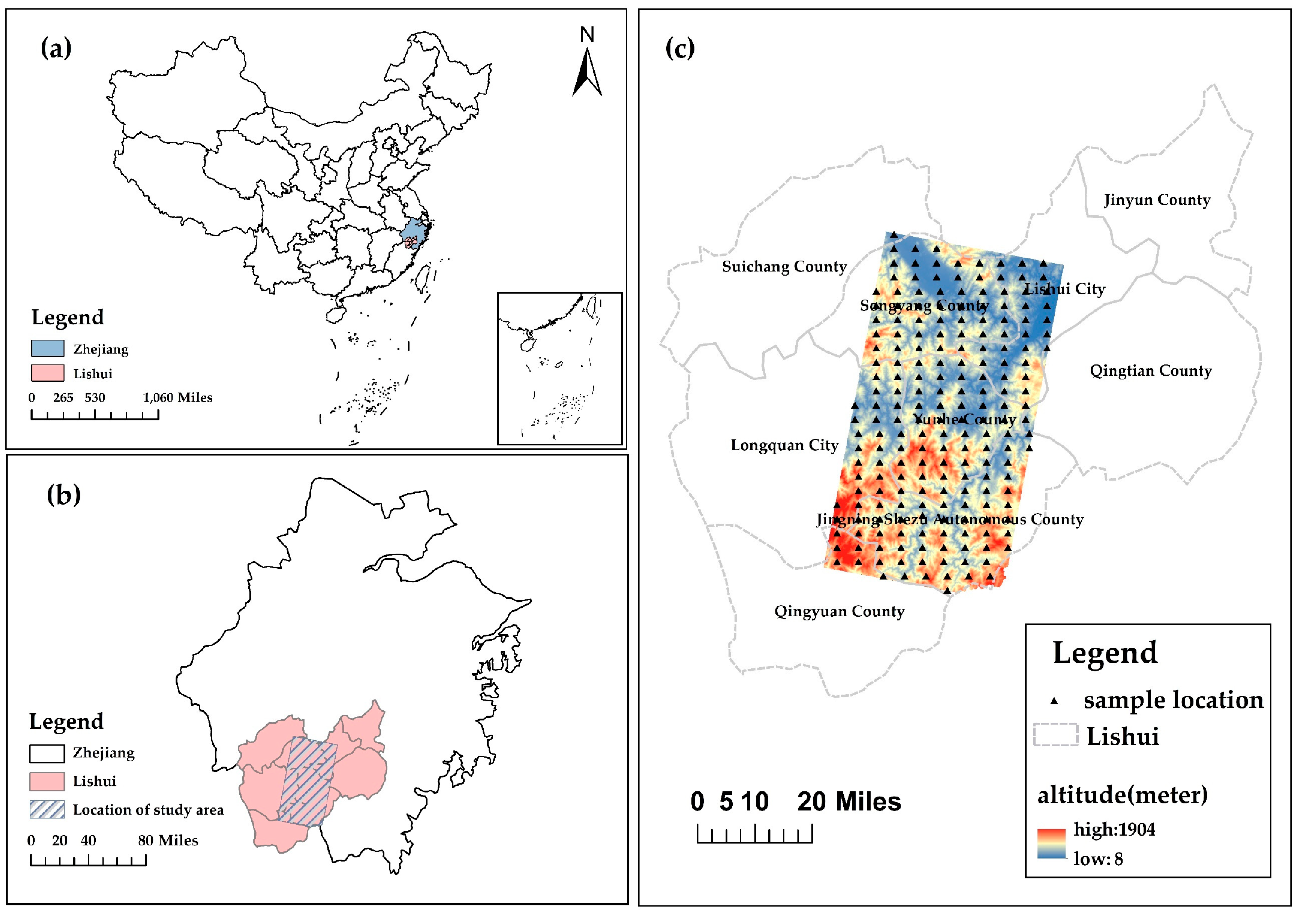
Figure 1. Maps of the study area. (a) Location of Lishui City, Zhejiang Province; (b) Location of the exact study site; and (c) Topography of the study area and locations of sample plots.
Forests 14 00526 g001
Figure 2. Schematic diagram of the downscaled image element changes influenced by predictor variable’s bandwidths:(a) Downscaling results with strong heterogeneity; (b) Smooth downscaling results.
Forests 14 00526 g002
Figure 3. The workflow of the analysis.
Forests 14 00526 g003
Figure 4. Importance of the top 15 variables (in terms of percentage increase of mean square error and increase in node purity).
Forests 14 00526 g004
Figure 5. Heat map of correlations between selected feature variables and AGB.
Forests 14 00526 g005
Figure 6. GWR and MGWR-identified bandwidths for different independent variable sets selected by different screening methods, including: (a) Random forest importance ranking; (b) Multiple stepwise regression; and (c) Pearson VIF.
Forests 14 00526 g006
Figure 7. MGWRD model training and validation performances: (a) Training samples (n = 118) and (b) Validation samples (n = 50).
Forests 14 00526 g007
Figure 8. AGB downscaling results based on the MGWR model.
Forests 14 00526 g008
Figure 9. Distribution histogram of the MGWRD-predicted AGB residuals.
Forests 14 00526 g009
Figure 10. Improved AGB predictions based on the MGWRD-CK model.
Forests 14 00526 g010
Table 1. Statistical summary of the post-filtering plots’ AGB values.
Number of Sample PlotsAGB (t/ha)Number of Samples Used
RangeMedianAverageStd DeviationTrainingValidation
16812.21–348.53174.28157.2671.4311850
Table 2. Multiple stepwise regression results.
Variable Selection AlgorithmFitting Equation
MSRY = 18.3836 + 0.27699 X 1 + 1.7721 X 2 + 1.7811 X 3 + 1.9741 X 4 − 7.1878 X 5 + 7.6935 X 6 − 2.3673 X 7 + 3.7678 X 8 − 1.5526 X 9 + 1.2759 X 10 + 1.6467 X 11 + 0.8492 X 12
Note: Y represents AGB; and X 1 , X 2 , X 3 , , X 11 are the slope, cor_B1_3, B15, EVI, sec_B4_3, aspect, var_B4_3, dis_B4_3, homo_B6_5, SAVI, B4, and mean_B5_3, respectively.
Table 3. Predictive performance indicators of OLS, RF, GWR, and MGWR applied to different independent variable sets identified using three variable screening methods.
Variable Screening MethodEvaluation Indicators
ModelRSSAICAICcCVR Square
Random Forest RankingOLS1390.85867.06932.8367.960.46
GWR348.55743.19873.2852.180.53
MGWR177.72382.75402.2348.890.58 *
RF567.34----59.870.52
Multiple Stepwise RegressionOLS1523.641070.951107.9395.540.32
GWR394.78966.36995.3368.910.43
MGWR282.45435.41451.8265.980.47 *
RF591.21----74.640.44
Pearson-VIFOLS1693.491146.131183.1180.880.30
GWR418.831166.421226.1583.630.44
MGWR289.19438.98476.1378.280.45
RF650.28----89.460.43
Note: RSS = residual sum of squares; AIC = Akaike information criterion; AICc = corrected Akaike information criterion; CV = coefficient of variation; R square = coefficient of determination. (* indicates statistical significance at the 5% level).
Table 4. Simulated semi-variogram models under OK and CK simulation strategies and their descriptive statistics.
Kriging
Method
Semi-Variogram ModelsNuggetSillNugget/SillRange/mR2RSS
OKExponential176.19320.870.55102930.788291
Spherical182.23289.740.6184640.6110922
Gaussian156.39269.640.58127320.749687
CKExponential153.24289.130.53111400.817963
Spherical176.59294.320.6088330.6310862
Gaussian162.32275.120.59123200.749375
Note: R2 is the fitting accuracy of the internal model of the semi-variance function.
Table 5. Accuracy validation statistics of the MGWRD-OK and MGWRD-CK models based on the validation data set.
ModelMAE(t/ha)RMSE/(t/ha)R2Bias/(t/ha)
MGWRD13.0216.230.58−2.74
MGWRD-OK12.0316.020.59−2.23
MGWRD-CK10.6215.380.62−1.69
Disclaimer/Publisher’s Note: The statements, opinions and data contained in all publications are solely those of the individual author(s) and contributor(s) and not of MDPI and/or the editor(s). MDPI and/or the editor(s) disclaim responsibility for any injury to people or property resulting from any ideas, methods, instructions or products referred to in the content.